An Operational Scheme for Deriving Standardised Surface Reflectance from Landsat TM/ETM+ and SPOT HRG Imagery for Eastern Australia

Abstract

Operational monitoring of vegetation and land surface change over large areas can make good use of satellite sensors that measure radiance reflected from the Earth’s surface. Monitoring programs use multiple images for complete spatial coverage over time. Accurate retrievals of vegetation cover and vegetation change estimates can be hampered by variation, in both space and time, in the measured radiance, caused by atmospheric conditions, topography, sensor location, and sun elevation. In order to obtain estimates of cover that are comparable between images, and to retrieve accurate estimates of change, these sources of variation must be removed. In this paper we present a preprocessing scheme for minimising atmospheric, topographic and bi-directional reflectance effects on Landsat-5 TM, Landsat-7 ETM+ and SPOT-5 HRG imagery. The approach involves atmospheric correction to compute surface-leaving radiance, and bi-directional reflectance modelling to remove the effects of topography and angular variation in reflectance. The bi-directional reflectance model has been parameterised for eastern Australia, but the general approach is more widely applicable. The result is surface reflectance standardised to a fixed viewing and illumination geometry. The method can be applied to the entire record for these instruments, without intervention, which is of increasing importance with the increased availability of long term image archives. Validation shows that the corrections improve the estimation of reflectance at any given angular configuration, thus allowing the removal from the reflectance signal of much variation due to factors independent of the land surface. The method has been used to process over 45,000 Landsat-5 TM and Landsat-7 ETM+ scenes and 2,500 SPOT-5 scenes, over eastern Australia, and is now in use in operational monitoring programs.

1. Introduction

The Australian states of Queensland, New South Wales and Victoria cover the whole of eastern mainland Australia, with an area of approximately 2.8 million km², or 161 scenes of Landsat-5 TM imagery. Since 1995, Queensland has used Landsat-5 TM and Landsat-7 ETM+ imagery to map land cover change [1], back as far as 1988. More recently, New South Wales and Victoria have begun similar vegetation monitoring programs [2], using Landsat and also SPOT-5 HRG imagery. All these programs have made use of biophysical indices calculated from the imagery [3–5], in a largely automated processing framework.

More generally, such monitoring of vegetation and land surface characteristics using satellite imagery depends on relationships between biophysical quantities on the ground and the spectral radiance measured by the satellite sensors. These relationships may be used implicitly, such as in the use of image classification techniques, or explicitly, as when calculating vegetation indices or other biophysical proxies. In either case, the result can be degraded by the presence in the imagery of variation which is not related to variation on the land surface [6,7].

Variation in measured radiance, caused by factors other than variation in the land surface, reduces the accuracy of the derived vegetation cover estimates if not accounted for. These factors include atmospheric conditions, sun and sensor positions, and surface orientation. A change in atmospheric conditions, or sun and sensor elevations (and hence path through the atmosphere) will alter the amount of light scattered and absorbed by the atmosphere. These changes affect both the amount of light illuminating the surface and the amount of light reaching the sensor. The topography and land cover affect how light illuminates and is reflected from the surface, as a function of the relative locations of the sun and the sensor.

Assuming the sensor radiometrics are well characterised, as is the case for Landsat-5 TM, Landsat-7 ETM+ [8] and SPOT-5 [9], then obtaining accurate vegetation cover retrievals from satellite imagery requires reducing the variation caused by atmospheric conditions, topographic and bi-directional reflectance effects. The aim of the work outlined in this paper was to develop a preprocessing scheme for deriving standardised surface reflectance from Landsat and SPOT imagery. The use of atmospheric radiative transfer models to remove atmospheric effects from Landsat imagery has been demonstrated in an operational context by a number of other authors, such as Masek et al.[10], Schroeder et al.[11] and Vicente-Serrano et al.[12], although the Australian landscape presents further challenges due to the lack of dark targets used for estimating atmospheric aerosol loading. Further variation could be removed if the imagery were also corrected for the effects of the bi-directional reflectance distribution function (BRDF), and topographic orientation. Roy et al.[13] and Li et al.[14] have shown schemes for doing this, and more recently Li et al.[15] have included topographic corrections, although both schemes rely on parameters derived from the MODIS sensor, which precludes their use prior to the launch of the Terra satellite in December 1999.

With the opening of the Landsat archive [16], and the consequent availability of much larger volumes of imagery, there is an increasing need for methods which can be applied without manual intervention.

The processing scheme described here combines widely accepted models of atmospheric and reflective processes with some parameterisation for the Australian land surface, to create a surface reflectance product adjusted to a standard viewing geometry of sun and satellite angles. It is simple enough to implement within an operational environment where thousands of images are to be processed. It requires no manual intervention, and can be applied to the entire record of imagery for the sensors under consideration.

Table 1. Mathematical Symbols.

Symbol	Meaning
ρ	Bi-directional reflectance factor
ρdif	Reflectance factor illumination by diffuse light only
γ	Ratio of reflectances from different angular configurations
β	Ratio of ρ to ρdif
L	Surface-leaving radiance
Edir	Direct irradiance on surface. Subscript h for a horizontal surface
Edif	Diffuse irradiance on surface. Subscript h for a horizontal surface
i	Incidence angle. Angle between surface normal and vector to sun
e	Exitance angle. Angle between surface normal and vector to satellite
ω	Relative azimuth. Angle between projections of the vectors to sun and satellite onto terrain surface
Vd	Sky view factor
Vt	Terrain view factor
Kvol	Volumetric scattering kernel of RossThick-LiSparse-R BRDF model
Kgeo	Geometric shadowing kernel of RossThick-LiSparse-R BRDF model
fiso, fvol, fgeo	Parameters for RTLSR BRDF model
f′vol, f′geo	Normalised RTLSR parameters, divided by fiso
θi, θv	Sun and satellite zenith angles, respectively

defines the mathematical symbols used in this paper.

2. Methods

2.1. Outline

The physical process being modelled can be summarised as follows: incoming solar irradiance passes through the atmosphere, reflects off the Earth’s surface, passes through the atmosphere again and is observed by the satellite sensor above the atmosphere.

Atmospheric effects on the signal include a range of scattering and absorption processes, and are a function of the various angles relating the sun, surface and satellite. These effects are assumed to be well modelled by widely available atmospheric radiative transfer models. We have used Second Simulation of the Satellite Signal in the Solar Spectrum (widely known as 6S) [17] for this component. This is described in more detail in Section 2.2.

Reflection from the Earth’s surface is also a function of the angular configuration of the sun, surface and satellite. The surface is characterised by the proportion of light it reflects, but this depends on the angles at which it is illuminated and viewed. The terminology for different reflectance quantities used here is that defined by Martonchik et al.[18]. When not otherwise specified, we have used the term “reflectance” to mean the bi-directional reflectance factor.

The atmospheric modelling with 6S yields an estimate of the surface reflectance assuming a horizontal surface. We have then modelled the effects of the bi-directional reflectance distribution function (BRDF) to estimate the surface reflectance for a surface oriented as per the topography for each pixel, as it would be if viewed with a standard illumination and viewing geometry. This we refer to generically as standardised surface reflectance. This is described in more detail in Sections 2.3 and 2.4.

2.2. Atmospheric Radiative Transfer Modelling

The atmospheric radiative transfer modelling software, 6S [17], provides estimates of direct and diffuse irradiance onto a horizontal surface, $E_h^{\mathit{dir}}$ and $E_h^{\mathit{dif}}$ respectively. 6S also provides estimates of apparent surface bi-directional reflectance, ρ_h, for a horizontal surface, given the observed top of atmosphere radiance. The top of atmosphere radiance was obtained from the satellite imagery by applying the supplied gains and offsets to each pixel digital number. All of these quantities are specific to the wavelength in question, but for notational clarity we have omitted the explicit band dependency in what follows.

6S was run at a range of angle combinations, with the resolution of angle change (in radians) being 0.01 for sun zenith, 0.02 for satellite zenith and azimuth, and 0.04 for sun azimuth. 6S was also run for a range of altitudes, for each angle combination, with an altitude step size of 200 m starting at sea level up to the maximum ground elevation required. Each pixel is then corrected using the resulting 6S parameters for the nearest corresponding elevation and angles. Ozone concentration was taken from the Total Ozone Mapping Spectrometer (TOMS) monthly climatology (1996–2003) [19]. Precipitable water was estimated by a simple regression from interpolated daily surface humidity measurements [20]. Aerosol optical depth (at 550 nm wavelength) was assumed to be a fixed value of 0.05, for the reasons discussed by Gillingham et al.[21], most notably the difficulty in obtaining accurate estimates of it directly from imagery over the relatively bright Australian landscape. Australia is frequently blessed with sufficiently clear skies that this is reasonable for the purposes of monitoring vegetation cover [22]. Aerosol was assumed to follow the continental aerosol model available in 6S. Surface elevation was given by the Shuttle Radar Topography Mission (SRTM), at 30 m resolution [23–25].

6S includes some capacity for modelling BRDF, but since it does not allow for a non-horizontal surface, we chose not to use this. We did this by setting it to use a homogeneous surface, with no directional effects, i.e. a uniform Lambertian surface. This effectively “switches off” BRDF modelling within 6S, leaving us free to model it separately.

2.3. Standardised Reflectance

The bi-directional reflectance factor is a measure of how much light the surface would reflect, when illuminated from a single direction, and observed from some particular direction. While this is a measure of how reflective the surface is, it does vary with the illumination and viewing geometry [18]. Expressing the reflectance of a pixel as a function of this geometry gives the bi-directional reflectance distribution function (BRDF). This function depends on the sub-pixel scale scattering and shadowing behaviour of the surface. Since the illumination and viewing geometry do vary between acquisitions of satellite imagery, this represents an extra source of variation in the measurements. To remove this extra variation, we seek to express the surface reflectance as it would be observed if seen under a standard configuration (i.e., a standard set of azimuth and zenith angles for both sun and satellite). We refer to this as standardised reflectance. For operational purposes we have standardised to a nadir view (i.e., satellite zenith angle is zero) and a solar zenith angle of 45°. This is also commonly known as Nadir BRDF-Adjusted Reflectance (NBAR) at 45°.

The output of 6S is an estimate of the surface bi-directional reflectance factor for a horizontal surface, ρ_h. However, as discussed above, we have switched off 6S’s BRDF modelling, so we must still apply a correction for this, for the angles appropriate for the orientation of the given pixel. The simplest approach is to define the ratio between reflectances at two sets of angles A and B

$$\gamma \left(A,B\right)=\frac{\rho \left(B\right)}{\rho \left(A\right)}$$

(1)

If we have a reflectance at angles A, and we can estimate γ(A, B) (using a model of BRDF), then we can estimate the reflectance at angles B as

$$\rho \left(B\right)=\gamma \left(A,B\right)\rho \left(A\right)$$

(2)

This general approach has been used successfully by other authors [13,26,27]. However, while this approach works well on horizontal surfaces, it performs less well as the terrain slopes further away from the sun. This is due at least in part to the reduced importance of direct illumination, and the increased importance of diffuse illumination. So, following Shepherd and Dymond [28], we take a slightly more complicated approach.

We define a second reflectance factor ρ^dif, the diffuse reflectance, which is similar in character to the hemispherical-directional reflectance factor defined by Martonchik et al.[18], but considering only the diffuse irradiance, with no direct illumination. We then assume that the surface-leaving radiance (in a given direction) can be modelled as

$$L=\frac{\rho E^{\mathit{dir}}+{\rho }^{\mathit{dif}}{E}^{\mathit{dif}}}{\pi }$$

(3)

Since 6S does not directly supply an estimate of the surface-leaving radiance, only the surface reflectance for a horizontal surface, we approximate the observed surface-leaving radiance L from the outputs of 6S (ρ_h, $E_h^{\mathit{dir}}$ and $E_h^{\mathit{dif}}$) as

$$L_{\mathit{obs}}=\frac{{\rho }_h\left(E_h^{\mathit{dir}}+E_h^{\mathit{dif}}\right)}{\pi }$$

(4)

This represents the actual radiance leaving the pixel, in the direction of the sensor, regardless of the orientation of the surface.

Following Shepherd and Dymond [28], the direct and diffuse irradiances illuminating a sloping surface can be written in terms of the irradiances illuminating a horizontal surface

$$E^{\mathit{dir}}=E_h^{\mathit{dir}}\frac{\text{cos}i}{\text{cos}{i}_h}$$

(5)

$$E^{\mathit{dif}}=E_h^{\mathit{dif}}{V}_d=\left(E_h^{\mathit{dir}}+E_h^{\mathit{dif}}\right)V_t{\rho }_{\mathit{avg}}$$

(6)

where i is the incidence angle between the surface normal and the sun vector; i_h is the incidence angle for a horizontal surface (i.e., the solar zenith angle); V_d is a sky-view factor; V_t is a terrain view factor; and ρ_avg is the average reflectance of surrounding pixels. V_d and V_t describe (in relative terms) how much sky and terrain are visible to the sloping pixel surface, to serve as a source of diffuse illumination. E^dir is set to zero when i ≥ 90°. Equation (5) is just the usual correction for sun angle (widely known as a cosine correction), and Equation (6) expresses the diffuse illumination as the sum of the diffuse light coming from the sky, and that reflected from surrounding terrain. No account is taken of the orientation of the surrounding terrain, and whether it would be directing light onto the pixel in question.

The sky view factor, V_d, is the proportion of sky visible to a given pixel, relative to a hemisphere of sky which would be visible if no surrounding terrain obstructed the view. The hemisphere can be thought of as having its base aligned with the slope of the pixel. The sky view factor was calculated using the horizon search methods detailed by Dozier and Frew [29]. For each pixel, the angle to the horizon is found in 16 equally spaced search directions, and a sky view factor along that azimuth is computed. The sky view factor for the whole hemisphere is approximated as the average of these 16 azimuthal view factors. The terrain view factor, V_t, is assumed to be whatever remains of the hemisphere over the slope at that point, thus V_t = 1 − V_d. The sky view factor, V_d, was pre-computed for every pixel, using the Shuttle Radar Topography Mission (SRTM) digital elevation model (DEM) at 30 m resolution.

The slope and aspect of the terrain are calculated directly from the 30 m SRTM using Fleming and Hoffer’s algorithm, as described by Jones [30]. This means that the effective resolution of the slope is 90 m, as it uses a 3 × 3 pixel window.

Solving Equation (3) requires an estimate of the diffuse reflectance. This seems likely to be closely related to the direct reflectance, so it was modelled as directly proportional to the direct reflectance [28].

$${\rho }^{\mathit{dif}}=\beta \rho$$

(7)

Shepherd and Dymond [28] modelled this with a constant β, but we have chosen to model β as a function of the angles, by integrating the BDRF model over the hemisphere. This is detailed in Section 2.4.

Using Equation (2), we define a reflectance correction factor γ_std to adjust a reflectance from a given set of angles to a standard angular configuration

$${\rho }_{\mathit{std}}={\gamma }_{\mathit{std}}\rho$$

(8)

Substituting Equations (7) and (8) into Equation (3) gives

$$L=\frac{\frac{{\rho }_{\mathit{std}}}{{\gamma }_{\mathit{std}}}\left(E^{\mathit{dir}}+\beta E^{\mathit{dif}}\right)}{\pi }$$

(9)

which we can rearrange to

$${\rho }_{\mathit{std}}=\frac{{\gamma }_{\mathit{std}}L\pi }{E^{\mathit{dir}}+\beta E^{\mathit{dif}}}$$

(10)

This gives an estimate of the bi-directional reflectance factor for a surface at a standard angular configuration. We can substitute L = L_obs from Equation (4), and E^dir and E^dif from Equations (5) and (6) respectively. The only remaining unknowns are γ_std and β, which are modelled using the BRDF model, as described in Section 2.4.

2.4. Topographic and Bi-Directional Reflectance Modelling

The viewing geometry varies with the sun and satellite positions, relative to the pixel under observation, and also with the orientation of the pixel surface, due to topography. We have chosen to model both these variations with a single BRDF model. This implicitly assumes that canopy roughness is the same for both horizontal and inclined surfaces. Laboratory work by Dymond and Shepherd [31] suggests that this may be valid, at least for closed canopies.

The kernel-driven RossThick-LiSparse reciprocal (RTLSR) BRDF model was chosen as it has been found to perform well for a range of land cover types [32], and has been used very successfully with data from the MODIS instrument [27,33].

This is expressed in terms of two kernel functions K_vol and K_geo, and three parameters f_iso, f_vol and f_geo

$$\rho =f_{\mathit{iso}}+f_{\mathit{vol}}{K}_{\mathit{vol}}\left(i,e,\omega \right)+f_{\mathit{geo}}{K}_{\mathit{geo}}\left(i,e,\omega \right)$$

(11)

where i, e and ω are the incidence, exitance and relative azimuth angles respectively [34]. (Note that the relative azimuth is calculated about the surface normal, so for sloping pixels this is not the same as the difference between the sun and satellite azimuth angles. This distinction disappears if the kernels are expressed in terms of phase angle.)

When used with the MODIS sensor, the model can be parameterised on a per-pixel basis. This is possible because each pixel is observed from multiple directions at multiple sun angles over a short time period (twice daily, typically over 16 days). The short time period means that there is very little variation on the ground itself, and so all variation is assumed to be due to the angular configuration. The range of angular configurations can be used to invert the model to provide a set of parameters which characterise the BRDF, for that pixel, in that 16 day period.

However, this is not possible with the Landsat or SPOT sensors. Because their orbits are sun-synchronous, the overpass time is roughly the same each day, and so the sun position does not vary in the short term. In the case of Landsat, the view geometry is also constant for each pass, so in general any given pixel is always viewed from the same angle. In the case of SPOT, the sensor is pointable, and so multiple view angles are possible, if image capture is appropriately tasked, although it would be difficult to obtain a large number of such views within a short period.

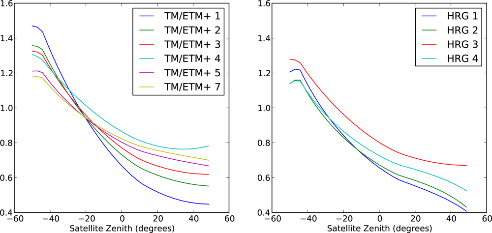
Because of these limitations, we have made the assumption that there is at least a major component of the BRDF which can be assumed to be the same across all pixels. This assumption is supported by the validation presented in Section 2.7. This global BRDF can be characterised with a single set of model parameters, which are then used for all pixels. There would, of course, remain a component of BRDF effect which is specific to each pixel, which we are not able to address with this approach. The correction for BRDF effects will only be successful in areas that satisfy the assumption that this global BRDF is the major component. With this assumption in place, we can address the orbital limitations of Landsat and SPOT by noting the following points:

• Areas in the overlap between two Landsat paths are viewed with different view angles;
• Images which are chosen to be within a few weeks of each other but across the equinoxes (Mar 21 & Sep 23) will have the largest range of sun zenith angles for the shortest time period, thus minimising on-ground change;
• Pixels on hill slopes will have different sun and view angles to horizontal pixels.

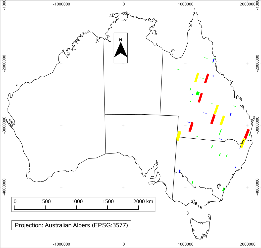
By selecting pairs of pixels in overlap areas, between dates chosen as above, on a range of pixel surface orientations, we obtain a set of pairs of reflectances across a whole range of angular configurations. Pixels in shadow, or with sun incidence angle >80°, were excluded because the BRDF model is believed to perform poorly at these extremes (it tends to infinity as incidence angle approaches 90°). In the case of SPOT we selected pairs of images which were taken off-nadir from opposite view directions. We also selected pixels across a range of land cover types, as represented by the foliage projective cover (FPC) class, and a range of slope classes. The image overlap locations were chosen to cover a number of the different land types in eastern Australia, to avoid being biased by any particular type of land surface. A total of 12,000 pixels were selected for parameter fitting for Landsat TM, and 10,400 for SPOT.

Because of our assumption of a global BRDF we did not attempt to solve Equation (11) for a full set of parameters. Rather, we solved for a ratio of reflectances, which would model the γ parameter we need. Combining Equations (1) and (11)

$$\begin{array}{lll}\gamma \left(A,B\right)\hfill & =\hfill & \frac{{\rho }_B}{{\rho }_A}\hfill \\ \hfill & =\hfill & \frac{f_{\mathit{iso}}+f_{\mathit{vol}}{K}_{\mathit{vol}}\left(i_B,e_B,{\omega }_B\right)+f_{\mathit{geo}}{K}_{\mathit{geo}}\left(i_B,e_B,{\omega }_B\right)}{f_{\mathit{iso}}+f_{\mathit{vol}}{K}_{\mathit{vol}}\left(i_A,e_A,{\omega }_A\right)+f_{\mathit{geo}}{K}_{\mathit{geo}}\left(i_A,e_A,{\omega }_A\right)}\hfill \end{array}$$

(12)

Because we solve only for this ratio, it is necessary to cancel out the f_iso parameter in order to guarantee a unique solution for the parameters. So, we define f′_vol = f_vol/f_iso and f′_geo = f_geo/f_iso and so

$$\gamma \left(A,B\right)=\frac{1+f_{\mathit{vol}}^{\prime }{K}_{\mathit{vol}}\left(i_B,e_B,{\omega }_B\right)+f_{\mathit{geo}}^{\prime }{K}_{\mathit{geo}}{i}_B,e_B,{\omega }_B)}{1+f_{\mathit{vol}}^{\prime }{K}_{\mathit{vol}}\left(i_A,e_A,{\omega }_A\right)+f_{\mathit{geo}}^{\prime }{K}_{\mathit{geo}}\left(i_A,e_A,{\omega }_A\right)}$$

(13)

For each pair of pixel observations we have an instance of Equation (2), and we solve the whole set together to give a single set of parameters f′_vol and f′_geo. The inversion process is detailed in Section 2.6. This is done independently for each wavelength, for each instrument. The resulting f′_vol and f′_geo, together with Equation (13), gives us a correction factor γ(A, B) to adjust a reflectance from any set of angles to any other set of angles.

2.5. Modelling β

The parameters f′_vol and f′_geo give us a function

$$R\left(i,e,\omega \right)=1+f_{\mathit{vol}}^{\prime }{K}_{\mathit{vol}}\left(i,e,\omega \right)+f_{\mathit{geo}}^{\prime }{K}_{\mathit{geo}}\left(i,e,\omega \right)$$

(14)

Because we have cancelled out the f_iso parameter, R is not a reflectance, but it has the same BRDF shape as reflectance. We can use this to model the ratio γ, with Equation (13), and also to model the ratio β. If we assume that the diffuse irradiance is isotropic, we can say that the surface is illuminated by separate sources in each part of the sky. Since ρ^dif is the reflectance for diffuse illumination only, we assume that the radiance leaving the surface in a given direction is the sum of the radiances reflected in that direction from each separate source. Thus ρ^dif can be expressed as the average of the direct reflectances for all combinations of incidence and relative azimuth angles

$${\rho }^{\mathit{dif}}\left(e\right)=\frac{1}{jk}\sum _{i=0}^{\pi /2}\sum _{\omega =0}^{2\pi }\rho \left(i,e,\omega \right)$$

(15)

where the summation steps are chosen to give equal area on the surface of the hemisphere. If we use R from Equation (14) to model the BRDF shape then we have

$$R^{\mathit{dif}}\left(e\right)=\frac{1}{jk}\sum _{i=0}^{\pi /2}\sum _{\omega =0}^{2\pi }R\left(i,e,\omega \right)$$

(16)

and so β can be modelled as

$$\beta \left(i,e,\omega \right)=R^{\mathit{dif}}\left(e\right)/R\left(i,e,\omega \right)$$

(17)

2.6. Inverting f′_vol and f′_geo

The inversion of the two parameters f′_vol and f′_geo was carried out by optimising over the pairs of observations of pixels. For each pixel in the training set, we have two observations of that pixel, ρ_A and ρ_B, within a few weeks of each other. We are assuming that there has been no on-ground change in that time, and so we should be able to use our BRDF model to adjust the reflectance from one set of angles to the other. We define ρ_B,A as being ρ_B adjusted to the angles for ρ_A. Equation (10) can be used to do this, using the angles for view A in place of the standard angles. So, over the set of training pixels, we optimise f′_vol and f′_geo, by minimising a total difference D

$$\begin{array}{lll}D\hfill & =\hfill & \sum _{\forall \mathit{pixels}}\left|{\rho }_A-{\rho }_{B,A}\right|\hfill \\ \hfill & =\hfill & \sum _{\forall \mathit{pixels}}\left|\frac{{\mathit{L}}_{\left(\mathit{obs},\text{A}\right)}\pi }{E_A^{\mathit{dir}}+{\beta }_A{E}_A^{\mathit{dif}}}-\frac{\gamma \left(A,B\right)L_{\left(obs,B\right)}\pi }{E_B^{\mathit{dir}}+{\beta }_B{E}_B^{\mathit{dif}}}\right|\hfill \end{array}$$

(18)

The ratios γ and β are re-calculated at each evaluation of D. Optimisation was carried out using the Nelder–Mead simplex algorithm available in SciPy [35].

2.7. Validation of BRDF Modelling

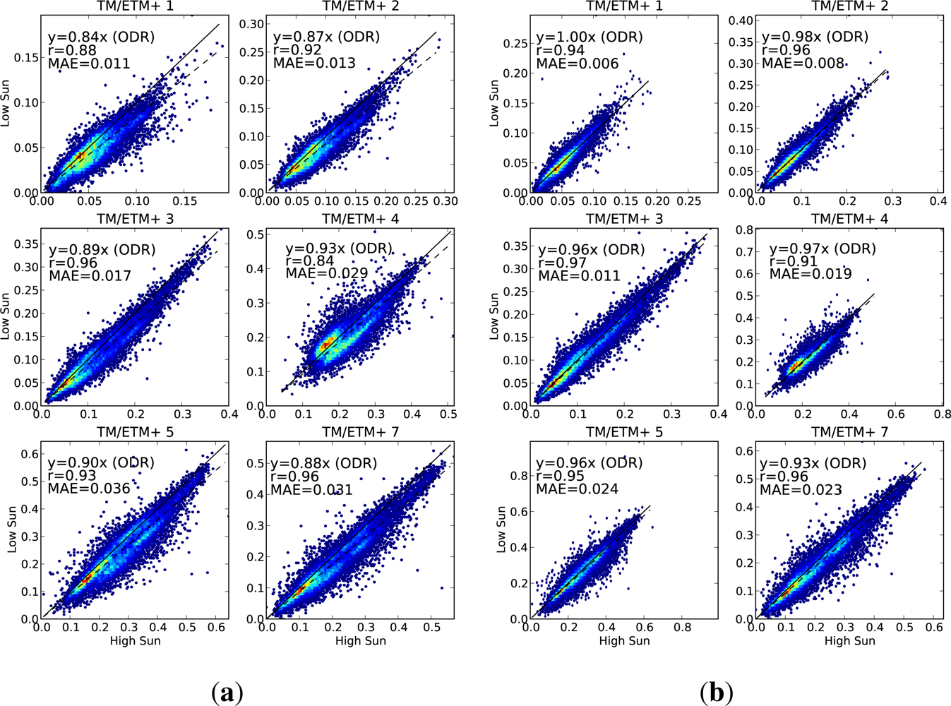
To test the value of the BRDF correction, we used paired observations of a second set of pixels, chosen in the same way as those used for parameter fitting, as described in Section 2.4. Following the same logic as used to fit the parameters, the fitted BRDF model should be able to adjust the reflectance from one set of angles to the other. The selection of pixels allows us to test the correction on a large range of angular configurations.

Given a pair of reflectances ρ_A and ρ_B, for a pixel, observed from two different sets of angles A and B, we can adjust ρ_B to the angles A. As in Section 2.6, ρ_B,A is ρ_B adjusted to the angles for ρ_A. We can treat this pair (ρ_A, ρ_B,A) as an observed-predicted pair, and assess the performance of the prediction accordingly. The extent to which they are equal gives a measure of the merit of the correction.

We have presented validation scatter plots for a wide range of situations, as experience has suggested that a poorly tuned parameterisation can perform well on one or two of these situations, but badly on others. Scatter plots are presented for the following cases.

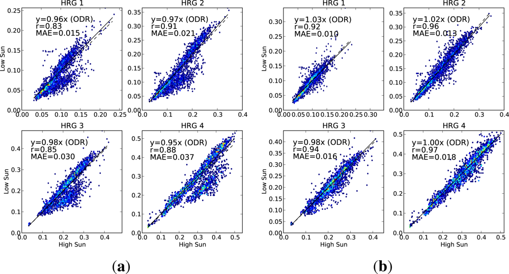
• Case 1. Landsat pixels on a mixture of horizontal and sloping terrain, with sloping pixels in a range of orientations, and some with and some without tree cover. This dataset has a large range of incidence/exitance angle combinations, on a range of land cover types. Pairs are divided into the low-sun and high-sun observations, with the low-sun value being used to predict the high-sun value. This tests how well we correct for the difference in sun angle. Sample size = 20,217 pixels (9,459 Landsat-5, 10,758 Landsat-7).
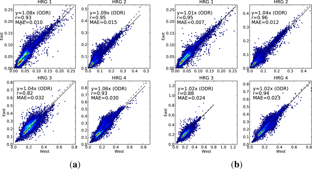
• Case 2. As for Case 1, but the pixels are split between the view from the east side of the overlap, and the view from the west side. The view from the east is used to predict the view from the west. This tests how well we are correcting for the difference in view angle. Sample size = 20,217 pixels (9,459 Landsat-5, 10,758 Landsat-7).
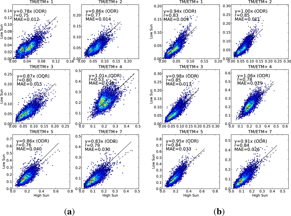
• Case 3. Landsat pixels on steep slopes facing away from the sun (slope > 50%, terrain aspect is within 60° of directly away from the sun). This is the situation when the diffuse illumination becomes important. Pairs are divided into low-sun and high-sun, and the low-sun value is used to predict the high-sun value. Sample size = 6,353 pixels (3,679 Landsat-5, 1,610 Landsat-7).
• Case 4. SPOT pixels on a range of orientations, split between high-sun and low-sun observations. Due to a limited number of overlap areas available with a large sun angle difference, other pairs were excluded from these plots (pairs used were those with Δθ_i > 10° from

  Table 5. The dates, locations and zenith angles for the overlapping pairs of SPOT imagery from which pairs of pixels were obtained for BRDF validation. Zenith angles in degrees, time difference in days. θ_i is sun zenith, θ_v is satellite zenith (both at scene centre).

  Lat/Long	Date	θi	θv	Lat/Long	Date	θi	θv	ΔTime	Δθi	Δθv
  −17.5/146.0	2006-07-04	47	16	−17.5/145.5	2006-08-05	45	−17	32	1	34
  −29.0/148.3	2005-07-28	57	−23	−29.0/148.4	2005-08-27	46	17	30	11	41
  −19.5/145.7	2009-06-09	48	25	−19.5/146.1	2009-08-01	48	−7	53	0	33
  −23.0/143.2	2005-07-16	53	−16	−23.0/142.8	2005-09-05	38	16	51	15	32
  −26.5/142.8	2009-09-27	36	−12	−26.5/142.8	2009-11-12	22	17	46	14	29
  −25.5/145.2	2009-08-16	47	18	−25.5/145.4	2009-10-08	32	−17	53	15	35
  −25.0/149.1	2009-07-01	57	−18	−25.0/149.6	2009-05-31	53	14	31	3	32
  −33.9/142.2	2009-04-14	53	−14	−33.9/141.6	2009-03-18	43	14	27	9	29
  −29.5/152.1	2009-05-16	56	−16	−29.5/151.5	2009-04-20	48	13	26	8	30
  −32.4/151.8	2009-03-04	40	−5	−32.4/151.2	2009-02-01	32	17	31	8	22

  ). This tests the correction for sun angle change, for the SPOT sensor. Sample size = 2,367 pixels.
• Case 5. SPOT pixels as for case 4, but including all overlap pairs. Pixels divided into those viewed from the east, and those viewed from the west. The view from the east is used to predict the view from the west. Sample size = 12,278 pixels.
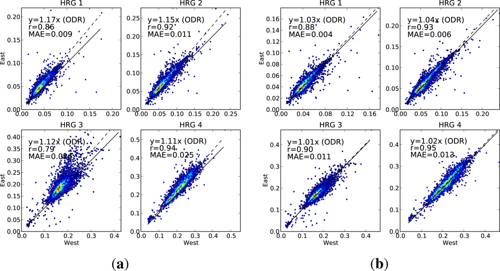
• Case 6. SPOT pixels from scenes pointed well off nadir view, from opposite sides, but within only a few days of each other. The largest date gap is 5 days, so we can reasonably assume no on-ground change, but the view angle differences are much larger than is possible with Landsat. This provides a more challenging test of the correction for view angle, because of the larger view angle difference, and with data less contaminated by possible change in vegetation between dates. Sample size = 4,117 pixels.

On each scatter plot, we include three measures of the performance. The linear correlation (r) is used to measure how closely related the observed and predicted values are. We also fit a regression line (using orthogonal distance regression (ODR), because there is equal uncertainty in both variables) and constrain it to pass through the origin. The slope of this regression line is a measure of any bias between the observed and predicted values. The third measure of performance is the mean absolute error (MAE), showing the absolute difference, in reflectance units, between the observed and predicted values. A perfect prediction would have both the correlation and the regression slope being equal to 1, and the mean absolute error would be zero.

For each of the cases, we present scatter plots for the data with no BRDF adjustment alongside the same scatter plot for the adjusted data, showing the extent to which the agreement is improved by applying the BRDF correction.

2.8. NDVI Improvement

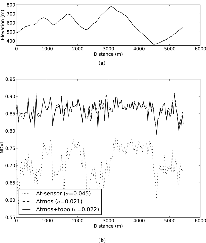
The ratios of spectral reflectances provide an opportunity to test the atmospheric correction. In particular, the normalised difference vegetation index (NDVI) is, on the one hand, strongly affected by relative offsets between the red and near infra-red bands, but is relatively stable under variation in illumination. Since one effect of the atmosphere is to increase the amount of radiance at the sensor by different amounts in different wavelengths (so-called path radiance), correcting for atmospheric effects will remove this path radiance offset and improve the stability of NDVI [36].

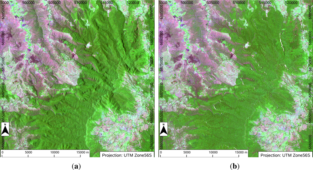
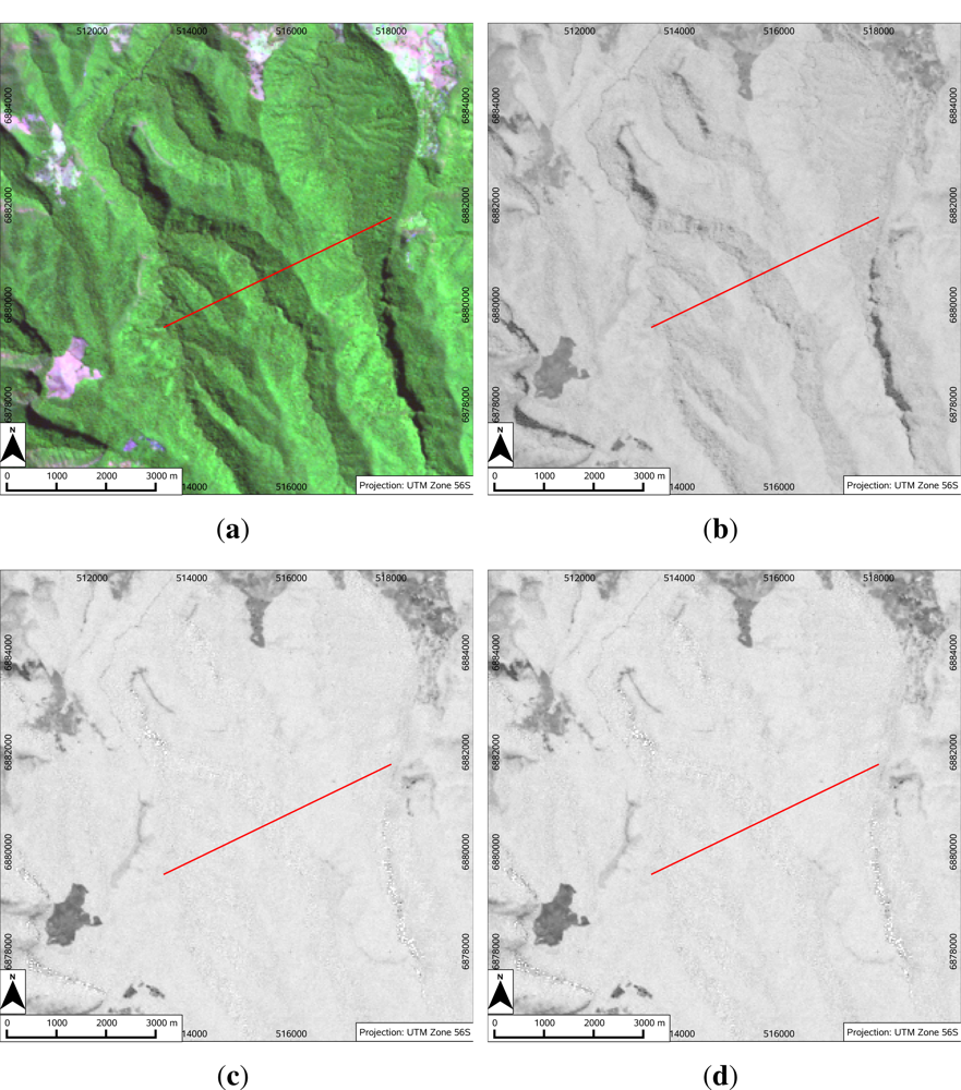
If NDVI is calculated from at-sensor reflectance values, this path radiance is still present in the signal and reduces the resilience of the NDVI to illumination changes. We can see this effect as topographic variation in NDVI when calculated from at-sensor reflectances.

A transect is defined through an area of apparently homogeneous forest, with marked topographic variation in illumination along the transect. Values along this transect are extracted from images of at-sensor reflectance, atmospherically corrected reflectance and standardised, topographically corrected reflectance. NDVI is calculated for each of these cases, and the result plotted against distance along the transect, to show how NDVI is affected by the different stages in the correction process, and by implication the effect of the correction on the relative magnitudes of the spectral reflectances. The corresponding imagery is also presented.

3. Data

All the Landsat imagery discussed was downloaded from the United States Geological Survey’s Earth Explorer website ( http://earthexplorer.usgs.gov), as level 1T processed scenes. All SPOT-5 imagery used was supplied commercially by Astrium Services (and is copyright CNES 2012), as level 1a products, and ortho-rectified by commercial contractors. All calibration coefficients and other metadata used were those supplied with the imagery.

Two sets of image pairs were selected, according to the criteria given in Section 2.4. One set was used exclusively for fitting the parameters f′_iso and f′_geo, while the other set was used for validation of the BRDF correction. The images in the validation set were all located in different regions to those used for parameter fitting. Every effort was made to select cloud-free imagery.

The date and location pairs chosen are shown in

Table 2. Landsat training pairs. The dates, locations and sun zenith angles (θ_i) for the overlapping pairs of Landsat imagery from which pairs of pixels were obtained for parameterising the BRDF model. Zenith angles in degrees, time difference in days.

		High-Sun			Low-Sun
Sensor	Row	Date	Path	θi	Date	Path	θi	ΔTime	Δθi
TM	079	2004-05-04	089	55	2004-02-21	090	41	73	14
TM	079	2004-08-24	089	51	2004-10-02	090	38	39	12
TM	079	2004-04-20	096	52	2004-02-24	095	41	56	10
TM	078	2003-08-18	093	53	2003-10-12	094	36	55	16
TM	078	2005-04-17	093	49	2005-02-19	094	38	57	10
TM	074	2003-09-09	096	43	2003-10-19	095	32	40	10
TM	074	2009-04-27	095	46	2009-03-01	096	37	57	9
TM	076	2003-09-01	095	47	2003-10-11	096	35	40	11

–

Table 6. The dates, locations and zenith angles for the overlapping pairs of SPOT imagery from which pairs of pixels were obtained for validating the extreme off-nadir correction. Zenith angles in degrees, time difference in days. θ_i is sun zenith, θ_v is satellite zenith (both at scene centre).

Lat/Long	Date	θi	θv	Lat/Long	Date	θi	θv	ΔTime	Δθi	Δθv
−17.5/145.0	2006-08-04	43	16	−17.5/145.5	2006-08-05	45	−17	1	2	34
−23.0/149.0	2009-08-01	49	20	−23.0/149.1	2009-08-02	51	−16	1	2	36
−23.0/149.5	2009-07-27	52	−19	−23.0/149.0	2009-08-01	49	20	5	3	40
−26.5/147.1	2009-06-16	58	−16	−26.5/147.0	2009-06-15	56	19	1	1	35

.

Points were generated in random sets across the landscape, stratified so that different FPC classes were equally represented. No pixel with incidence angle greater than 80° on either date was used. Each image was then checked for cloud or shadows affecting the pixel locations, and those points were removed from the selection.

Locations of overlaps used for training and validation are shown in Figure 1.

4. Results

4.1. BRDF Parameters

Table 7. Final parameters for BRDF model, for Landsat and SPOT.

Instrument and Band	f′vol	f′geo
Landsat TM/ETM+ 1	0.93125413991	0.260953557124
Landsat TM/ETM+ 2	0.687401438519	0.213872135374
Landsat TM/ETM+ 3	0.645033011917	0.180032152925
Landsat TM/ETM+ 4	0.704036740665	0.093518142066
Landsat TM/ETM+ 5	0.360201003097	0.162796996525
Landsat TM/ETM+ 7	0.290061903555	0.147723009593
SPOT-5 HRG 1	0.171683591728	0.302488786296
SPOT-5 HRG 2	0.00192651321278	0.295120586536
SPOT-5 HRG 3	0.551133247211	0.156266670124
SPOT-5 HRG 4	0.0703689039321	0.244430768625

gives the values of the parameters resulting from the parameter optimisation described in Section 2.6, for both Landsat and SPOT instruments. These parameters are used in Equations (13) and (14) to model γ and β respectively. The shape of a BRDF model is often reported as a graph of the function along the principle plane, with the sun at 45°, so for completeness we present those plots, for all bands, in Figure 2.

4.2. Validation of BRDF and Topography Correction

Figures 3–8 show the scatter plots for pairs of pixels under test cases 1 to 6. On all plots, the X axis shows reflectances which are not adjusted for BRDF, while the Y axis is the reflectance value from the other set of angles, either with or without adjustment to the angles for the X axis. The solid line is the 1-to-1 line, and the dashed line is the regression line (orthogonal distance regression), constrained to pass through the origin. The slope of the regression line gives a measure of systematic bias in the prediction. The colours represent the density of points on the scatter plot, from blue (lowest) to red (highest). For each set of scatter plots, there is one plot for each band for the sensor in question, i.e., six bands for Landsat TM/ETM+ and four for SPOT HRG.

Figure 3 shows the general case of correcting for BRDF on widely mixed terrain, for all 6 reflective bands of Landsat TM/ETM+. Figure 3(a) shows the relationship between reflectance measured at the two different sun angles, and clearly shows a systematic bias to give a lower apparent reflectance when the sun is lower in the sky. This is as one would expect, as the lower sun elevation means that sub-pixel structural elements cast longer shadows, and so the sensor sees more area in shadow. Figure 3(b) shows the effect of correcting for BRDF, with the slope of the regression lines closer to 1, and the correlation also increased. The mean absolute error is reduced in all bands. For the sake of brevity we have not shown the separate analysis of TM and ETM+, as the correction performs in much the same way for both sensors.

Figure 4 shows the effect of a different view angle in Landsat images. In Figure 4(a) the view from the east shows a higher apparent reflectance than the view from the west. This is because when the pixel is viewed from the east, the sun is behind the sensor, and so the sensor sees more of the sunlit side of sub-pixel structural elements than when viewed from the west. Figure 4(b) shows this effect is reduced after correction for BRDF, with much better agreement between the two views.

Figure 5 shows the effect of decreased illumination on the hill slopes facing away from the sun. In Figure 5(a), the uncorrected reflectances are markedly lower when the sun is lower, but figure 5(b) shows that after correction for BRDF, the agreement between the reflectances at different sun angles is much improved.

Figure 6 tests the correction for sun angle with the SPOT sensor. Much less data was available than for Landsat, and the effect is not so clearly systematic as with Landsat, because of the much greater view angle difference also present in these pairs, but as with Landsat, the correlation and the regression slope are both brought closer to a value of 1, showing an improvement in the agreement between the two views of the surface.

Figure 7 tests the correction of SPOT imagery for view angle effects, over all the overlap areas from Table 5, covering a range of land types across eastern Australia. As with Landsat, the agreement between reflectance from different views is improved by the BRDF correction.

Figure 8 shows the correction for more extreme view angles available with the SPOT pointable sensor. This case is worthy of separate consideration because the time gaps between pairs of images are limited to only a few days, and therefore there is very little likelihood of any change on the surface. The other main source of variation is from BRDF effects. The regression slopes in the uncorrected plots are in the range 1.11 to 1.17, but in the corrected plots they are between 1.01 and 1.04, which shows considerably better agreement between the two views.

Figure 9 shows a region in South East Queensland. In Figure 9(a) the image is standardised without allowing for topography (i.e., using only the sun and satellite angles for horizontal terrain). In Figure 9(b) the image is standardised using the angles appropriate for the terrain at each pixel. The removal of the topographic effects is apparent. Areas in shadow, or with incidence angle >80°, are masked and show as white in Figure 9(b).

Figure 10 shows a mosaic of Landsat TM images chosen from the period Aug–Oct 2006, for eastern Australia. This period covers the spring equinox, during which sun angle changes most rapidly with date. The images were selected to be as free as possible of cloud, but also alternately selected from the early or late end of the time period for adjacent paths. This means that there is fairly large variation in sun elevation between adjacent images. This time of year is in the late dry season for northern Australia, but moreover, it was during a period of prolonged drought in most of eastern Australia. The implication of this is that there would have been minimal change in the vegetation during that period. This selection of images means that we can see noticeable variation in at-sensor reflectance, evident as visible scene boundaries (Figure 10(a)) which is probably not due to real variation on the ground. Figure 10(b) shows the same imagery after correction to surface reflectance. The scene boundaries are almost completely invisible.

4.3. NDVI Improvement

Figure 11(a) shows an area of apparently homogeneous forest, across terrain with slopes facing towards and away from the sun, with clear differences in illumination (path/row 089/080, date 2011-09-13). The red line is a transect across this terrain, sampling these areas of different illumination. Visually, this forest appears to be of fairly constant density along the transect, and so one would expect the NDVI to be fairly constant as well.

Figure 11(b–d) shows the NDVI calculated over this region, using different levels of reflectance correction. Figure 11(b) shows NDVI calculated from at-sensor reflectance. It shows notable residual variation from topographic illumination differences. Figure 11(c,d) shows NDVI calculated from corrected reflectance, where Figure 11(c) has been corrected for atmospheric and BRDF effects, but without removing topographic effects, and Figure 11(d) is fully corrected for topography as well. Both of these latter images show almost no apparent effect of topographic illumination variation in the NDVI signal.

Figure 12 shows the variation of NDVI along this transect (from south-west to north-east), for different levels of radiometric correction. The standard deviation of NDVI along the transect is given as σ on the graph. These show that the atmospheric correction has removed most of the variation in NDVI due to illumination differences, and the final topographic correction provides very little further improvement. This suggests that the removal of the path radiance from the signal has brought the red and NIR bands into the correct proportion, making the resulting NDVI very resilient to illumination variation.

5. Discussion

The BRDF validation plots show that we have removed substantial amounts of the variation due to the angular configuration and BRDF effects. For almost every case presented, the prediction of reflectance from one angular configuration using reflectance from another configuration is greatly improved by using the BRDF modelling described. This improvement is measured in terms of the correlation between the two reflectances, in terms of the regression relationship between them, and in terms of the mean absolute error. In all cases, at least one of these measures improved with the BRDF adjustment, and in most cases all measures improved. In all plots, the mean absolute error was improved by the BRDF correction.

The plots in Figures 3–8 show that different types of angular effects have been removed, including variation due to view angle, sun angle and surface orientation.

The NDVI plots suggest that we have improved the relative magnitudes of the reflectances at different wavelengths. It also suggests that vegetation indices calculated from surface reflectance would be substantially more resistant to variation in illumination than when calculated using at-sensor reflectance.

The reflectance imagery in Figure 9 shows very clearly the removal of topographic effects. Areas which appear on the uncorrected image to be of homogeneous vegetation, but illuminated differently due to topography, appear in the corrected image as having almost uniform reflectance.

The mosaic of surface reflectance in eastern Australia in Figure 10(b) shows very little evidence of the visible scene boundaries which appear in the at-sensor reflectance mosaic (Figure 10(a)). This almost complete removal of scene boundaries suggests that the corrections are performing equally well across most of eastern Australia.

Because of the global nature of the BRDF correction, there will remain some variation due to BRDF effects which are specific to the land cover at each pixel. This is probably the major remaining source of variation present in the scatter plots. Further analysis would be required to investigate whether any method of parameterising BRDF at a more local scale (e.g., per pixel or per landtype) would be able to improve on the BRDF corrections achieved with the current fixed average BRDF shape.

Other sources of variation would include actual change on the ground, minor registration errors between images, and limitations in the resolution of the DEM used to calculate slope. The final point would be important in areas such as along ridge lines and steep valley floors, where the slope and aspect change sharply over short distances, and would be particularly important for the SPOT cases, because of the smaller pixel size of the SPOT-5 HRG instrument (10 m). However, in most areas, the slope calculated from the 30 m SRTM appears to be sufficiently accurate.

Due to limitations on available inputs to the atmospheric modelling, some atmospheric effects will remain. In particular, imagery captured on days with high aerosol loading will be less accurate in the shorter wavelengths. Fortunately, such days are more rare in Australia than in some parts of the world.

There seems no reason why this method would not be equally applicable to the rest of Australia, given that atmospheric conditions and land surface types are broadly similar. However, before applying the method to other parts of the world, some assumptions would need to be checked. In particular, the assumption of a fixed, low value for aerosol optical depth would not be valid everywhere, and other methods may be needed to estimate aerosol loading. Also, it is possible that the land surface structure in other parts of the world may be fundamentally different to that in Australia, and the BRDF parameterisation may need to be re-fitted for different regions. This could be tested using the same methods presented here.

It also seems feasible that the same methods could be applied equally well to other similar instruments, assuming the availability of sufficient overlapping image pairs covering a suitable range of angular configurations to parameterise the BRDF model.

6. Conclusions

By combining existing methods for atmospheric and BRDF correction with some tuning for Australian conditions, a practical operational method has been developed for calculating standardised surface reflectance for Landsat TM/ETM+ and SPOT-5 HRG sensors.

Atmospheric correction was performed using a widely accepted model of radiative transfer, with appropriate parameters for the Australian atmosphere. Through careful choice of image dates, pairs of overlapping images were selected, which allowed us to also parameterise the effects of the bi-directional reflectance distribution function (BRDF), for each sensor wavelength, in a manner that can be applied equally well to the whole data record for the sensors in question. For all wavelengths and geometric configurations considered, the errors due to BRDF are shown to be reduced by application of this BRDF correction, with the mean absolute error being reduced, in many of the cases described, by as much as 50% of the error in the uncorrected data.

This method has been readily applied to an archive of some 45,000 Landsat images, and 2500 SPOT images, and the resulting surface reflectance imagery is now in use by the relevant Queensland, New South Wales and Victorian state government agencies for vegetation monitoring programs.