Comparing Urban Impervious Surface Identification Using Landsat and High Resolution Aerial Photography

Abstract

This paper evaluates accuracies of selected image classification strategies, as applied to Landsat imagery to assess urban impervious surfaces by comparing them to reference data manually delineated from high-resolution aerial photos. Our goal is to identify the most effective methods for delineating urban impervious surfaces using Landsat imagery, thereby guiding applications for selecting cost-effective delineation techniques. A high-resolution aerial photo was used to delineate impervious surfaces for selected census tracts for the City of Roanoke, Virginia. National Land Cover Database Impervious Surface data provided an overall accuracy benchmark at the city scale which was used to assess the Landsat classifications. Three different classification methods using three different band combinations provided overall accuracies in excess of 70% for the entire city. However, there were substantial variations in accuracy when the results were subdivided by census tract. No single classification method was found most effective across all census tracts; the best method for a specific tract depended on method, band combination, and physical characteristics of the area. These results highlight impacts of inherent local variability upon attempts to characterize physical structures of urban regions using a single metric, and the value of analysis at finer spatial scales.

1. Introduction

Urbanization is arguably one of the most significant landuse/landcover change occurring in the world today [1,2]. Sizes and distributions of urban areas are dynamic because of rising populations. In 2009, for the first time in history, the percentage of human population that lived in urban areas exceeded 50%—the United Nations estimates this percentage will increase to 69% by 2050 [3]. Although urban expansion is often attributed to increasing population, the rate of conversion to urban land uses far exceeds the rate of urban population increase, a phenomenon common across the world [3].

Conversion to urban land—losses of agricultural and forested lands, coupled with increasing impervious surface cover—has direct effects on natural temperature regulation [4,5] and alters the hydrologic cycle [5–7]. Decreasing vegetative cover and increasing impervious surface cover alters thermal processes in urban regions, thus creating warmer temperature regimes relative to rural areas (urban heat island effect) [5,8,9]. Alteration of the hydrologic cycle represents the most significant urban water quality issue present today [5,6,10] because stormwater runoff from impervious surfaces creates water quality problems including higher water temperatures and elevated levels of contaminants in surface waters [5,11]. A better understanding of such impacts is required to effectively address these adverse issues [5,10,12].

Mapping impervious surfaces is essential for evaluating these impacts and implementing effective environmental and urban management planning [5,10,12–17]. Since the 1970s, remote sensing has been widely used for analyses of urban areas [5,13,18,19]. The earliest research specifically devoted to impervious surface identification began in the 1990s, but was limited in scope until high-resolution imagery and increased computing power became available (in the mid-2000s) [13].

High-resolution imagery provides the spatial detail necessary to record the fine-scale heterogeneity present within an urban area [12,13,15,18,20–22]. Researchers readily acknowledge that this fine-scale heterogeneity is a problem for remote sensing, especially with regards to creating mixed pixels (pixels influenced by the variation in spectral values present within its dimensions). Ultimately, the solution to this issue lies in identification of analyses capable of resolving this fine detail. However, acquisition and analysis expenses, limited spatial extent, and high costs of sequential coverage limit routine applications.

Because of this heterogeneity, a wide variation in remote sensing techniques, image sources, and effectiveness exists from study to study [5,13,18], and creates a lack of uniformity that limits our ability to make comparisons between studies [5,18]. Furthermore, the success of each of the approaches is often evaluated in different ways, for example—accuracy assessments, root mean square error, absolute error, which presents obstacles for other researchers to effectively interpret the findings and identify the most effective method(s).

Despite the relatively coarse spatial resolution of Landsat imagery in the context of urban analysis (30 m by 30 m pixel size), it offers advantages of affordability, accessibility, multispectral coverage, sequential acquisition, and the spatial scope to represent complete urban systems. Much literature is specifically devoted to applications of Landsat imagery to derive impervious surfaces, however, assessing and comparing even this body of literature is very difficult. A selection of this literature is presented in

Table 1. Selected Studies, using Landsat imagery, that illustrate the variety of classification techniques to identify impervious surfaces.

Method as Identified in Paper	Location (Image Date) [Reference]
Artificial neural networks	State of Connecticut, USA (1995) [10]; Central New York State, USA (2001) [24]
Linear segmentation	Bangkok, Thailand (1987) [25]
Subpixel analysis	Charleston, SC, USA (1990) [26]; DuPage and Cook Counties, IL, USA (1997) & East Greenwich, RI, USA (1997) [27]; State of Missouri, USA (1980, 1990 & 2000) [28]
Linear mixture analysis	Columbus, OH, USA (1999) [29]
NDVI	Atlanta, GA, USA (1979, 1987, &1997) [30]; Fairfax County, VA, USA (1990, 1995, & 2000) [31]; Montgomery County, MD, USA (1990–2001) [32] Tampa Bay, FL, USA (1991–2002) [33] Seattle-Tacoma, WA, USA (1986 & 2002) and Las Vegas, NV, USA (1984 & 2002) [34]; Cixi County, China (1987, 2000, 2002 & 2009) [35]
Regression tree	Sioux Falls, SD, USA (2000), Richmond, VA, USA (1999), and the Chesapeake Bay, USA (1999–2001) [23]; Western Georgia, USA (1993 & 2001) [36] Washington DC-Baltimore, MD, USA (1984–2010) [37]
Spectral mixture analysis	Columbus, OH, USA (1999) [38]; Marion County, IN, USA (2000) [39]; Lake Kasumigaura, Japan (1987, 2000, & 2007) [40] Franklin County, OH, USA (1999) [41]
Regression analysis with tassel cap	Twin Cities Metropolitan Area, MN, USA (1986–2000) [19]; State of Minnesota, USA (1990 & 2000) [42]; Franklin County, OH, USA (1999, 2000, & 2003) [43]
Support vector regression using sub-pixel classification	Germany (1999–2001) [44]
Object oriented classification and Normalized Difference Built-up Index	Jiaozuo, China (2007) [45]
Multi-layer perceptron neural network with support vector machine	Beijing, China (2009) [46]
Normalized Impervious Surface Index	Xiamen City, China (2009) [47]
Linear spectral unmixing	Pearl River Delta, China (1998, 2003 & 2008) [48]

([10,19,23–48]), which does not attempt a comprehensive review, but rather presents an illustration of the variety of techniques applied in many different areas. Only one of these studies evaluates the effectiveness of a multi-scale approach (from a finer scale to increasingly larger scales—see [23]). Very few have compared applications of alternative techniques within the same milieu (see [49–51]).

Therefore, the objective of this paper is to evaluate accuracies of selected image classification strategies, as applied to Landsat imagery. It will assess the effectiveness of Landsat data for mapping urban impervious surfaces by using a reference data set manually delineated from high-resolution aerial photos. We then evaluated the robustness of these strategies at a finer scale. Our goal is to identify the most effective method(s) for delineating impervious surfaces using Landsat imagery, and to determine if finer scale analyses are needed, thereby guiding applications for selecting cost effective delineation techniques for urban regions.

2. Methods

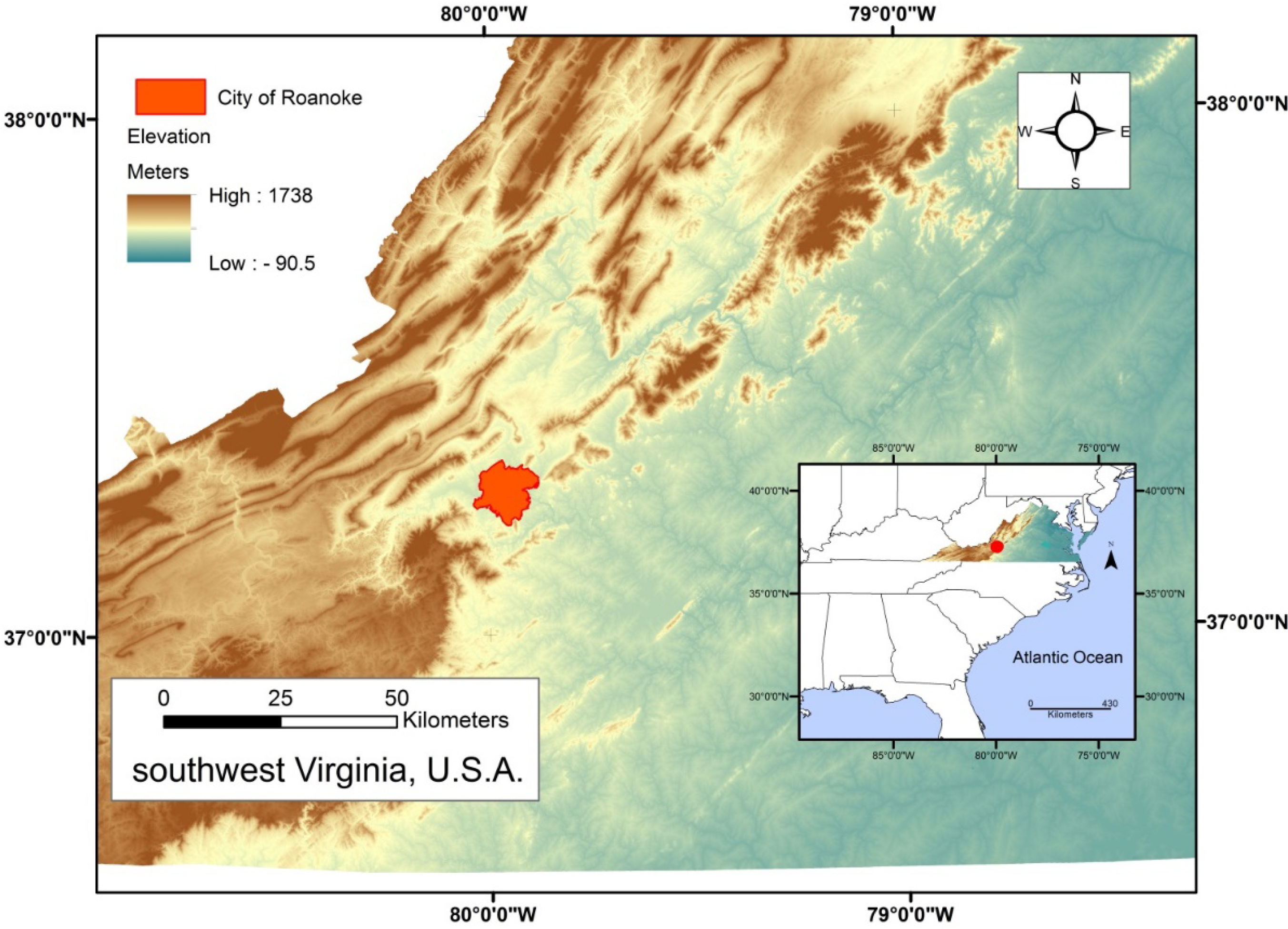
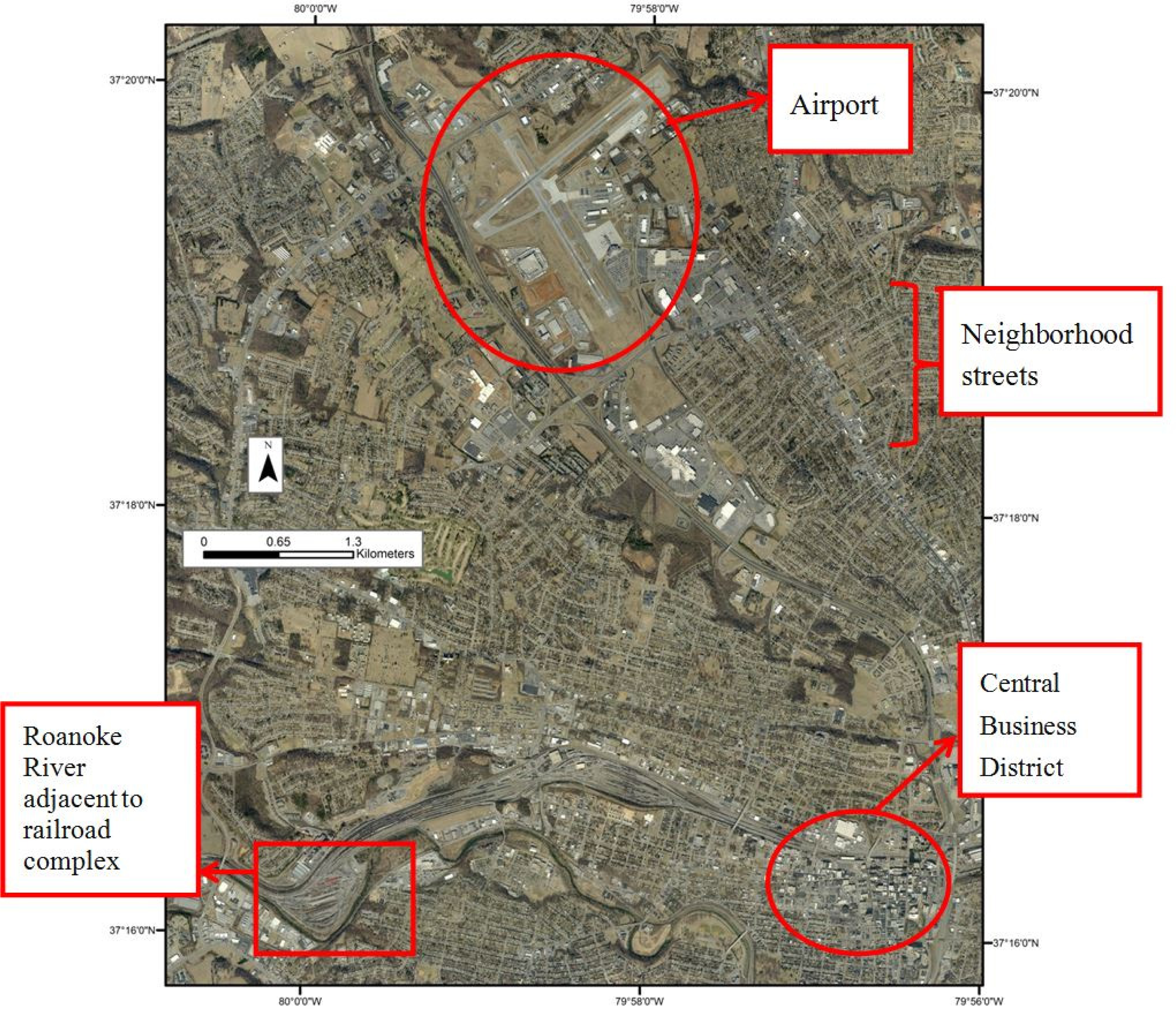
2.1. Study Site and Data

The study site is the City of Roanoke, Virginia, USA, a small city (110 square kilometers) located in a valley in southwest Virginia (Figure 1). Roanoke is the largest city in Virginia, outside of the major metropolitan areas in the eastern part of the Commonwealth. Although small in area, Roanoke has a population density comparable to much larger cities in the USA.

Over recent decades, Roanoke has been the focus of substantial urbanization, economic stress, and landuse changes. Roanoke has substantial drainage problems and experiences frequent flooding due to its proximity to the Roanoke River, the river’s tributaries, and urban stormwater runoff from impervious surfaces. Many segments of the Roanoke River system within the city are on the Virginia Department of Environmental Quality’s impaired waters list, due to contaminants such as Escherichia coli, high water temperatures, and heavy metals [52]. In addition, its CO₂ emissions were estimated at 2.3 million tons in 2009 [53], and city officials estimate impervious surface cover at 28% [54]. For our analysis, Roanoke offers the advantage of a compact urban region with a range of land uses and urban environments that permit evaluation of alternative analytical strategies.

2.2. Delineating Impervious Surfaces from Aerial Photos

GIS shapefiles—roads, buildings, and parcels—for our study site were downloaded from Roanoke’s geospatial data gateway and the US Census Tigerline data gateway. We accessed aerial photos through the Virginia GIS server with ESRI’s ArcCatalog^® GIS server connection. The Virginia Base Mapping Project 2011 flyover for the city occurred between 4 March 2011 and 10 March 2011 [55], completed with 6 inch resolution [56].

We overlaid the city’s boundary, parcels, and building shapefiles on the 2011 aerial photos, and, using them as guides, impervious surfaces were delineated in GIS. Many urban researchers have conducted their analyses using landuse or landcover boundary delineations, (see [9,57,58]; this strategy seems to be fruitful for studies that focus upon analysis of urban heat island, but is less well-matched for studies that must consider other dimensions of the urban landscape. For our analysis, impervious surface delineation was accomplished separately by each census tract because: (a) each census tract is spatially compact and contains different landuse/landcovers with varying percent impervious, (b) subdividing the study area provides the ability to evaluate intra-urban variations at a fine scale, and (c) providing impervious surface data individually by census tracts allows for consideration of impervious surfaces’ relationships with demographic data. Census tracts are spatial subdivisions delineated by the United States government for which statistical data is collected during the decennial census [59]. After editing roads and buildings shapefiles, we joined these using GIS, creating a single polygon for each census tract, then calculated percent impervious for each.

2.3. Landsat Image Processing

A cloud-free Landsat TM 5 scene (path 17, row 34, dated 13 March 2011) was obtained from the US Geological Survey’s GloVis server. The US Geological Survey provides the scenes with georeferencing already complete. The image was cloud-free and LEDAPS [58,60] preprocessing removed remaining atmospheric effects during preparation of the surface reflectance image. A histogram adjustment was conducted to ensure no negative reflectance values.

The image was subset to form multiple band combinations—bands 5, 6 and 7; bands 1, 5, and 7; and bands 2 through 6. We chose to include the thermal channel (band 6) because of impervious surfaces contribution to UHI [20–22], and bands 1, 5, and 7 as band 1 is useful for distinguishing soil from vegetation, and the spectral properties of impervious surfaces can mimic soil surfaces [61,62]. Supervised classification was performed on the entire scene for these three images and an image with all seven bands.

Training Areas of Interest (AOIs) were created separately for each band combination using a binary classification—impervious and other. Locations for the impervious surfaces’ training areas were identified using the aerial photos, typically including man-made objects such as the airport runways, parking lots, US Interstate highways, and large buildings—shopping malls/centers. Training areas for the other category included all pervious landcovers—agriculture, forests, water, and included several golf courses. We did not limit our training areas to Roanoke City but used the entire Landsat scene to avoid including mixed pixels, which were often problems near roads and for the city’s urban forest. We created AOIs for the other category using forested areas in the Jefferson National Forest (west and southwest of the City). We created AOIs for the impervious surfaces related to roads by using wider segments of the Interstate 81 corridor where the pavement has four or more lanes in each direction with little to no adjoining vegetation.

Using a feature space created separately from each image, we assessed the training data for normality, separability, and partitioning, and combined selected areas of interest as needed. These assessments ensured that brightness values for our different categories were not highly correlated, were mutually independent between bands, and that spatially separate pixels were not spectrally similar to each other. Our final signatures represented multiple different and distinct spectral classes for each of the two landcover categories—impervious and other. Four supervised classifications were performed on each image—parallelepiped, maximum likelihood, minimum distance, and Mahalanobis’ distance.

2.4. Validation Points and Accuracy Assessment

We created a validation dataset by generating a shapefile of random points for each census tract. The total number of random points for the entire city was 1,877—the numbers of samples positioned within census tracts varied from 50 in the smallest census tract to 115 in the largest. We overlaid these point files individually on the 2011 aerial photos and identified each point as either impervious or other.

The most widely utilized data set in the USA for impervious surfaces was developed by the Multi-Resolution Land Charateristics Consortium (MLRC) as part of the National Land Cover Database (NLCD). This raster dataset was developed to identify “percent developed imperviousness” for the coterminous USA [63]. The dataset was derived by means of regression tree software using both leaf-on and leaf-off Landsat images and images from NOAA’s Defense Meteorological Satellite Program [63]. The National Land Cover Database Impervious Surfaces (NLCD IS) dataset presents a continuous layer with a gradient of imperviousness from 0 to 100 percent for each 30 m by 30 m pixel [64], i.e., the value of each pixel is identified as the percent of impervious surfaces present within that pixel. Accuracy assessments have been performed on the full NLCD with resulting overall accuracies ranging from 59.7% to 80.5% [65], 43%–83% [66], and 78%–85% [67]. We were unable to locate a similar accuracy assessment performed specifically on the NLCD IS dataset.

Using the random points, we performed an accuracy assessment of the NLCD IS dataset representing our study area. After downloading the dataset from the MRLC website, we used GIS to generate several binary files with varying impervious thresholds from 10% to 75%, masking the extent to the city’s political boundary. We added each NLCD threshold file to the attribute tables of our random points shapefile, and calculated user’s accuracy, producer’s accuracy and overall accuracy for each threshold. We performed this assessment to establish a base threshold for overall accuracies of our classified Landsat images. Our method for this assessment differs from those employed by other researchers because we are assessing the presence or absence of impervious surfaces, whereas they calculated accuracies for all landcover/landuse categories (see [65–68])

The datum for Landsat Imagery is WGS 1984 and the datum for the NLCD is NAD 1983 Albers. So, for each classified image, we changed the spatial reference from WGS 1984 to NAD 1983 Albers so our accuracy assessments would be comparable to that of the NLCD IS data. We added the value of each pixel (impervious or other) for each classified image for each point to the random points’ attribute table, and then calculated overall accuracy for each image.

Our objective is to determine the most effective method(s) for identifying impervious surfaces from Landsat imagery. As such, as explained below and in table in Section 3.3, we chose the four classified images with the highest overall accuracies and compared those images to the aerial photos. We examined them visually to assess their effectiveness in delineation of specific landmarks, such as the airport, river, railway complex, neighborhood streets, and central business district (Figure 2) by comparing the results to our aerial photos.

2.5. Assessment of Accuracy at the Census Tract Scale

After choosing the images with the greatest overall accuracy for the entire study site, we then assessed accuracy variations within the urban system, using census tracts as units. Although census tracts form somewhat arbitrary units for investigating impervious surfaces, their use here supports related analyses in our study area, and provides boundaries with which governments and institutions are increasingly defining their urban space within the USA. We chose eleven contiguous census tracts within our study site to accomplish the assessment. These included the census tract with the smallest area (also the most highly developed as it comprises the central business district—Number 11), the largest in area (6.01), and the census tract with the least amount of development (28).

3. Results

3.1. Aerial Image Delineation of Impervious Surfaces

The percent impervious, as delineated from the aerial photos, for the eleven census tracts used in the finer scale analysis ranged from 13.3% (Tract 28) to 89.5% (Tract 11) (

Table 2. Percent impervious (IS) delineated from aerial photos and total area of census tract.

Census Tract No.	3	4	5	6.01	6.02	11	23	24	26	27	28
Percent IS	44.5	37.4	44.2	22.5	32.0	89.5	24.3	26.7	39.6	35.5	13.3
Hectares	883.3	359.6	354.3	1,106.1	599.8	105.3	789.7	283.9	159.2	415.1	1,077.5

). The smallest census tract (11), 105.3 ha, representing the central business district, has the largest percent impervious at 89.5%. Census Tract 28, with the smallest percent impervious (13.3%), is the second largest in area (1,077.5 ha).

3.2. Accuracy Assessments of the NLCD IS Data Set

For pixel impervious values ≥ 10%, the accuracies of the several binary classifications of the NLCD IS data resulted in overall accuracies ranging from 53.5% (pixel impervious value ≥ 10%) to 72.8% (pixel impervious value ≥ 45%) and kappas from 0.21 to 0.43 (

Table 3. Overall accuracy and kappa of Roanoke’s NLCD IS dataset at varying thresholds of percent impervious.

Impervious Threshold	Overall Accuracy	Kappa
10%	53.5%	0.21
35%	68.6%	0.39
40%	71.4%	0.42
45%	72.8%	0.43
50%	72.6%	0.39
75%	70.6%	0.25

). Accuracy and kappa increase as the threshold of impervious percent increases until about 40%–50%. Overall accuracies range between threshold values of 35% and 75%, and are consistently close to 70% or above. These results are consistent with the overall accuracy assessments completed on the general NLCD performed by other researchers (see [65–69]), and thus, form our baseline with which to compare our different classifications on the Landsat Images.

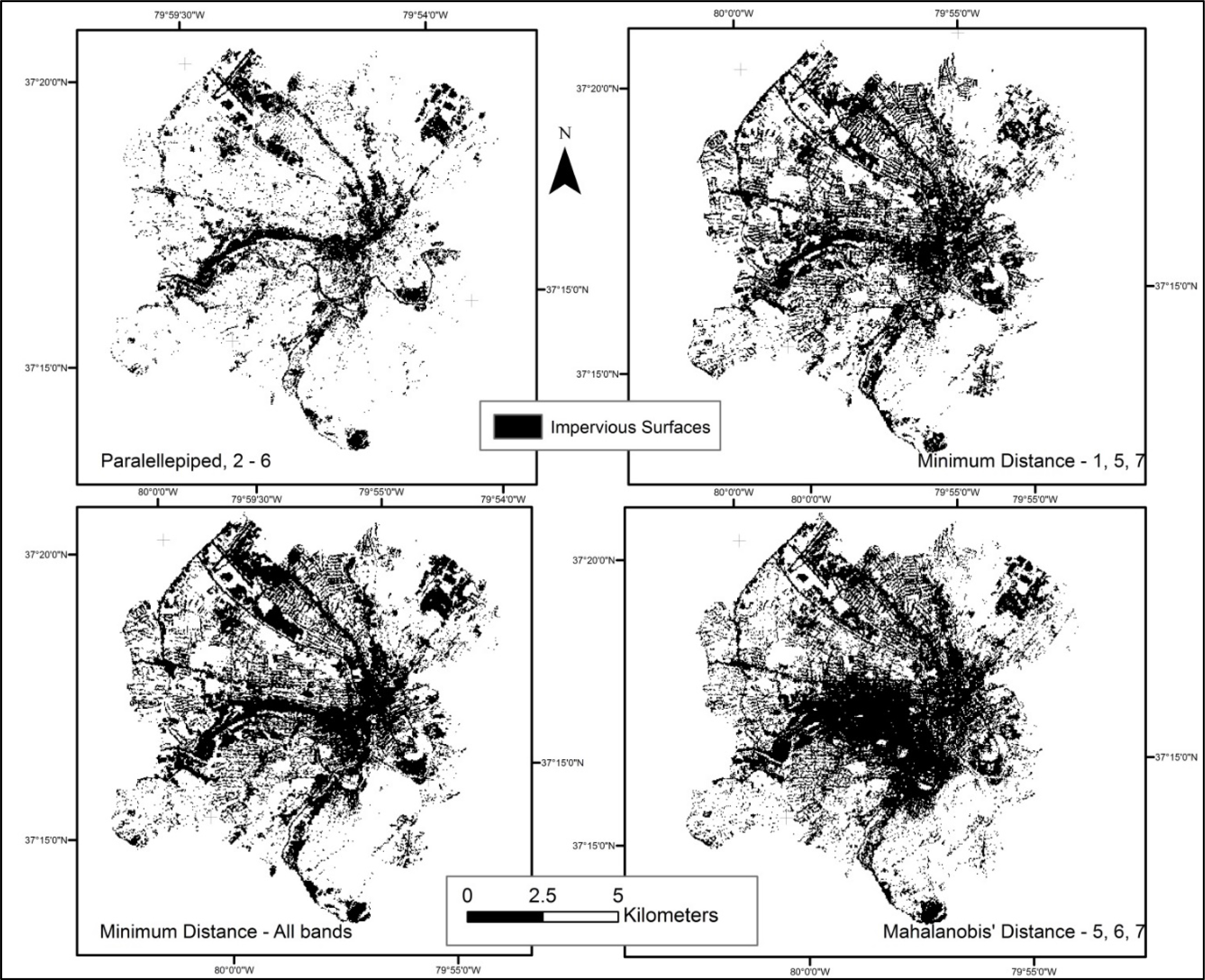
3.3. Accuracy Assessments of the Supervised Classifications

Overall accuracies for all sixteen supervised images ranged from 50.8% (Mahalanobis’ distance: all bands) to 72.1% (parallelepiped: bands 2–6) (

Table 4. Overall accuracy (OA) and kappa of all sixteen classified Landsat images^*.

Image and Classification	OA	Kappa	Image and Classification	OA	Kappa
All Bands			Bands 2–6
maximum likelihood	56.5%	0.22	maximum likelihood	68.3%	0.38
minimum distance	70.8%	0.39	minimum distance	67.6%	0.33
parallelepiped	64.4%	0.32	parallelepiped	72.1%	0.33
Mahalanobis’ distance	50.8%	0.16	Mahalanobis’ distance	68.6%	0.38
Bands 1,5, & 7			Bands 5, 6, & 7
maximum likelihood	59.8%	0.28	maximum likelihood	67.7%	0.35
minimum distance	71.1%	0.40	minimum distance	55.1%	0.18
parallelepiped	67.3%	0.36	parallelepiped	67.2%	0.32
Mahalanobis’ distance	61.8%	0.31	Mahalanobis’ distance	69.4%	0.38

Notes:

^*classified images in red were chosen for the finer scale analysis.

). Our kappa values for these classified images ranged from 0.16 (Mahalanobis’ distance: all bands) to 0.40 (minimum distance: bands 1, 5, and 7) (Table 4). All the classification methods using the band combination of channels 2–6 produced results similar to the NLCD IS standard. The results for ten of our sixteen classified images were comparable to results achieved for the NLCD IS (i.e., for pixel impervious values ≥ 10%, NLCD IS overall accuracies remained steady around 70% and the kappas for the NLCD IS around 0.40).

Since our objective was to identify the most effective method(s), we selected parallelepiped—bands 2–6; minimum distance—bands 1, 5, and 7; and minimum distance—all bands to include in our finer scale assessment at the census tract level. These three images had the highest overall accuracies and highest kappas. In addition, we had other several classified images that achieved results similar to the NLCD IS standard, so, we also chose to include the image which attained the highest overall accuracy and highest kappa—Mahalanobis’ distance—bands 5, 6, and 7. These selections gave us one classified image from each band combination and the four images for our finer scale assessment.

3.4. Comparison of Aerial Photos to Supervised Classifications

In this section, we are only reporting our visual assessment of the four classified images chosen in Section 3.3 above. Each of the images (Figure 3) provided sharp detail for the airport area, the major roads and highways, the railway complex, and a large shopping center near the airport. Minimum distance—bands 1, 5, and 7; minimum distance—all bands; and Mahalanobis’ distance—bands 5, 6, and 7 provide additional detail including most of the neighborhood streets. Minimum distance—bands 1, 5, and 7; minimum distance—all bands; and parallelepiped clearly record the high concentration of impervious surfaces within the central business district. Minimum distance—all bands performed the best in separating the river from the surrounding impervious surfaces, an area which can cause difficulty because of the many bridges crossing the river and sediments within the river from stormwater runoff. The neighborhood streets can cause difficulties with different classification algorithms because of shadowing from buildings and some trees, along with variations in width and types of adjoining vegetation.

3.5. Supervised Classification Results—Finer Scale

Table 5. Percent impervious for the manual delineation of aerial photos and percent impervious for each of the four chosen classification methods (Figure 3), and listed by census tract.

	Method
Census Tract No.	Aerial Photos	Parallelepiped (Bands 2–6)	Minimum Distance (Bands 1, 5 & 7)	Minimumdistance (All Bands)	Mahalanobis’ Distance (Bands 5, 6, &7)
	% IS*	% IS	% IS	% IS	% IS
3	44.5	36.4	49.5	59.1	53.7
4	37.4	19.3	55.3	52.5	52.4
5	44.2	25.2	59.8	58.1	69.3
6.01	22.5	17.3	24.6	30.1	29.3
6.02	32.0	23.0	39.2	39.8	39.0
11	89.5	84.0	93.8	96.6	92.7
23	24.3	12.8	33.6	33.5	26.2
24	26.7	5.2	40.4	36.8	53.4
26	39.6	29.0	61.2	61.3	67.1
27	35.5	24.3	56.4	52.2	58.6
28	13.3	7.5	18.2	14.3	17.9

Notes:

^*IS = impervious surface.

encapsulates the results from the manual delineation of the percent impervious for each census tract, and the percent impervious per census tract for each of the four chosen classified images (Figure 3). The divergence of the classified image percent from the manual delineation percent is enumerated in

Table 6. Difference in percent imperious between aerial photo delineation and classified images, listed by census tract^*.

Census Tract No.	Method
	Parallelepiped (Bands 2–6)	Minimum Distance (Bands 1, 5 & 7)	Minimum Distance (All Bands)	Mahalanobis’ Distance (Bands 5, 6, &7)
3	−8.1	5.0	14.6	9.2
4	−18.1	17.9	15.1	15.0
5	−19.0	15.6	13.9	25.1
6.01	−5.2	2.1	7.6	6.8
6.02	−9.0	7.2	7.8	7.0
11	−5.5	4.3	6.9	3.2
23	−11.5	9.3	9.2	1.9
24	−21.5	13.7	10.1	26.7
26	−10.6	21.6	21.7	27.5
27	−11.2	20.9	16.7	23.1
28	−5.8	4.9	1.0	4.6

Notes:

^*a negative value indicates an under-estimate.

(negative values indicate under estimates). Parallelepiped—bands 2–6 consistently under-estimated the percent impervious in all census tracts (a range in differences from −21.5 to −5.2) (Table 6). The other three methods over-estimated percent impervious for all census tracts (a range in differences from 1.0 to 27.5) (Table 6). No single method produced consistent under- or over-estimates in all the census tracts.

When examined at finer scale, no one method consistently provided the highest accuracies and kappas in all tracts. Overall accuracies and kappas for each of the four images by census tract were variable (

Table 7. Overall accuracy (OA) and kappa (k) for each of the four chosen classified images, listed by census tract.

Census Tract No.	Method
	Parallelepiped (Bands 2–6)		Minimum Distance (Bands 1, 5 & 7)		Minimum Distance (All Bands)		Mahalanobis’ Distance (Bands 5, 6, &7)
	OA	k	OA	k	OA	k	OA	k
3	76.7%	0.52	60.2%	0.21	66.0%	0.33	64.1%	0.29
4	57.9%	0.18	61.8%	0.23	56.6%	0.12	65.8%	0.31
5	70.7%	0.41	61.3%	0.21	68.0%	0.35	66.7%	0.31
6.01	81.7%	0.38	75.7%	0.31	75.7%	0.36	75.7%	0.39
6.02	76.7%	0.44	71.1%	0.40	74.4%	0.45	72.2%	0.39
11	78.0%	0.23	88.0%	0.34	86.0%	0.17	78.0%	0.03
23	78.4%	0.29	79.4%	0.49	73.5%	0.39	77.5%	0.38
24	69.1%	0.09	75.0%	0.47	73.5%	0.44	69.1%	0.40
26	64.9%	0.12	71.9%	0.47	68.4%	0.40	68.4%	0.41
27	65.8%	0.24	64.6%	0.28	65.8%	0.30	60.8%	0.24
28	85.8%	0.31	78.8%	0.21	82.3%	0.28	85.0%	0.47

), consistent with the percent impervious comparisons in Tables 5 and 6. However, in six of the census tracts, all four methods achieved accuracies similar to the NLCD IS standard. Two of our census tracts had accuracies that exceeded those standards—Tracts 11 and 28. Census Tract 11 has the highest percent impervious and both minimum distance images achieved accuracies in excess of 80.0%. Census Tract 28 has the lowest percent impervious; all methods achieved accuracies in excess of 78%. We did find two census tracts (4 and 27) where the overall accuracies were lower than the NLCD IS standard.

All classification methods produced overall accuracies equal to or exceeding results of the city-wide NLCD IS in the majority of the census tracts (parallelepiped bands 2–6 and minimum distance all bands in eight of eleven tracts, and the other two methods in seven of eleven tracts). The methods also produced overall accuracies in 18 of 44 assessments that exceed the city-wide NLCD IS standard (≥75%), and at least one kappa higher than the NLCD IS standard (≥0.43). In most cases, the highest overall accuracy and highest kappa for a specific census tract was from the same method, with three exceptions—Census Tracts 6.01, 6.02 and 28.

4. Discussion

For our study site, at least four of the supervised classification methods performed as well as the NLCD IS data set with respect to overall accuracy and kappa value at the coarser city scale. Three of our four most effective classifications were based in part upon the TM’s thermal channel, an effect that is consistent with reports of other researchers who have noted the contribution of the thermal channel to classification of impervious surfaces to the UHI [5,13,16,70]. Because our leaf-off imagery records a time with little to no vegetation growth (winter season), Band 1 was useful for distinguishing soil from vegetation especially in instances where impervious surfaces—roads, highways, parking lots—exhibit properties similar to bare earth (no vegetative cover) [5,61]. Visually, these four classifications did vary in effectiveness for identifying distinguishable features (especially neighborhood streets, the river, and the central business district) in various parts of the city. In certain heterogenic urban areas, such as these specific locales, the classification algorithms vary in their latitude to assign mixed pixels to specific spectral categories.

When examined at the finer detail of the census tract, internal heterogeneity within the city greatly impacted the results. Except for a few census tracts, our classifications produced variable results within and across the census tracts. Census tracts are defined by demographic criteria, so are not comparable to each other with respect to composition and variation in landuse/landcover.

With larger average parcel sizes, our accuracies are higher but in areas with wide variability in parcel sizes (thus greater heterogeneity) our accuracies were more variable across the methods.

Consideration of average parcel size within the census tract, spatial patterns of the parcels, percent impervious, and interactions with the classification algorithm, contribute to variability of results (

Table 8. Summary of census tract characteristics and best classification method for that census tract.

Census Tract No.	% IS Aerial Photos	Average Parcel Size (ha)	Range of Parcel Sizes (ha)	Highest Overall Accuracy	Highest Kappa	Best Classification Method
3	44.5	0.39	234.5	76.7%	0.52	parallelepiped, bands 2–6
4	37.4	0.14	6.0	65.8%	0.31	Mahalanobis’ distance (bands 5, 6, & 7)
5	44.2	0.12	6.3	70.7%	0.41	parallelepiped, bands 2–6
6.01	22.5	0.33	79.2	81.7%	0.39	parallelepiped, bands 2–6
6.02	32.0	0.26	26.7	76.7%	0.45	parallelepiped, bands 2–6
11	89.5	0.11	2.1	88.0%	0.34	minimum distance(bands 1, 5 & 7)
23	24.3	0.27	47.1	79.4%	0.49	minimum distance (bands 1, 5 & 7)
24	26.7	0.11	14.7	75.0%	0.47	minimum distance (bands 1, 5 & 7)
26	39.6	0.08	28.9	71.9%	0.47	minimum distance (bands 1, 5 & 7)
27	35.5	0.12	26.3	65.8%	0.30	minimum distance (all bands)
28	13.3	0.33	82.9	85.8%	0.47	Mahalanobis’ distance (bands 5, 6, & 7)

):

Parcels

• ▪ Parcel sizes, range of parcel sizes within a specific tract, the percent impervious, and the spatial pattern of land uses all affect accuracy;
• ▪ Units with very high and very low percent impervious show high accuracies for all methods (Census Tracts 11 and 28); and
• ▪ Units with the highest percentages of impervious surfaces (Census Tract 11), show low kappa values; the more variability in range of parcel sizes within a census tract and the higher percent impervious, the greater variability in accuracy of classifications between the methods.

Classification Strategy

• ▪ At least one classification method achieved an accuracy of over 70% in nine of the eleven census tracts;
• ▪ Parallelepiped classification—bands 2–6 proved the most effective method in tracts with moderate percentages of impervious surfaces and larger average parcel sizes;
• ▪ In some census tracts, multiple methods achieved accuracies higher results greater than the city-wide NLCD IS standard; and
• ▪ For all census tracts, the most effective method included either the thermal channel (band 6) or the blue visible channel (band 1).

Our analysis is subject to several sources of uncertainties:

Although we avoided bias in our random points dataset by retaining an independent party to complete it, human error still could have been a factor and some points misidentified between impervious or other;

Shadowing from buildings and coniferous trees could have altered brightnesses of some pixels resulting in misclassification between impervious and other;

For our finer scale analysis, we chose the best four methods from the broader scale analysis; so, it is possible that another method, which we did not consider, could have performed equally well or better at the finer scale analysis.

Some imprecision can occur when comparing point values to pixel values—our pixels cover a 90 square meter area; in urban settings, this area could encompass several different surface covers whereas a random point has no area and could be located anywhere within a pixel with different surface covers. Additionally, many studies have pointed out the problems encountered with mixed pixels within urban areas and have developed alternative methods in attempts to solve the mixed pixel dilemma [5,13]. However, our analysis indicates that more complicated methods in delineating impervious surfaces from Landsat imagery may not be necessary for this study site. Our overall accuracies at the coarser city-wide scale for several of our images were comparable to the overall accuracy of the widely used NLCD IS dataset, and to accuracies achieved by many of the more complex methods referenced in Table 1. At finer census tract scales, and even though no one method was effective across all census tracts, different methods and band combinations produced accuracies in excess of 70% and 80%.

5. Conclusions and Future Outlook

Based on our analysis, Landsat imagery is effective in delineating urban impervious surfaces using standard classification methods but the best specific method is highly dependent on the internal heterogeneity within a specific site. Most of our classifications at the city scale provided accuracies equivalent to that of the US National Land Cover Database. Our study shows that, for our study site and similar urban areas, a finer scale analysis using spatially compact boundaries can overcome this internal heterogeneity and provide higher accuracies. The best method will depend on physical characteristics of the finer-scale compact area.

The literature on identification of impervious surfaces is abundant, with the majority of the studies analyzing urban areas at coarse scales. To properly manage impacts of urbanization, such as stormwater mitigation and temperature regulation, analyses must account for the heterogeneity within urban regions. We encourage applications of more robust, and more detailed, reference data to permit analysis and validation at finer spatial scales to provide improved assessment, and to permit analysis of the detailed spatial fabric of the urban landscape.

Many developed countries have high-resolution aerial photos available to aid in identification of impervious surfaces. However, these analyses are not uniformly effective and derivation of impervious surfaces from high-resolution aerial photography is time-intensive and costly, a practical concern for developing countries. In contrast, the Landsat image archive is free, readily available for most regions of the world, and covers many decades. And, as our study reveals, standard classification methods can be quite effective especially when completed at finer scales.

References and Notes

1. Deelstra, T.; Girardet, H. Urban Agriculture and Sustainable Cities. In Growing Cities, Growing Food: Urban Agriculture on the Policy Agenda, a Reader on Urban Agriculture; Bakker, N., Dubbeling, M., Gundel, S., Sabel-Koschella, U., de Zeeuw, H., Eds.; Deutsche Stiftung für Internationale Entwicklung; Zentralstelle für Ernährung und Landwirtschaft: Feldafing, Germany, 2000; pp. 43–66. [Google Scholar]
2. Pickett, S.T.A.; Cadenasso, M.L.; Grove, J.M.; Nilon, C.H.; Pouyat, R.V.; Zipperer, W.C.; Costanza, R. Urban ecological systems: Linking terrestrial ecological, physical, and socieoeconomic components of metropolitan areas. Annu. Rev. Ecol. Syst 2001, 3, 127–157. [Google Scholar]
3. United Nations, World Urbanization Prospects: The 2009 Revision; Population Division, Department of Economic and Social Affairs, UN: New York, NY, USA, 2010.
4. Geiger, R.; Aron, R.H.; Todhunter, P. The Climate Near the Ground, 6th ed.; Rowman & Littlefield: Lanham, MD, USA, 2003. [Google Scholar]
5. Slonenecker, E.T.; Jennings, D.B.; Garafalo, D. Remote sensing of impervious surfaces: A review. Remote Sens. Rev 2001, 20, 227–255. [Google Scholar]
6. DeBusk, K.; Hunt, W.F.; Hatch, U.; Sydorovych, O. Watershed retrofit and management evaluation for urban stormwater management systems in North Carolina. J. Contemp. Water Res. Educ 2010, 146, 64–74. [Google Scholar]
7. Welker, A.L.; Wadzuk, B.M.; Traver, R.G. Integration of education, scholarship, and service through stormwater management. J. Contemp. Water Res. Educ 2010, 146, 83–91. [Google Scholar]
8. Oke, T.R. Initial Guidance to Obtain Representative Meteorological Observations at Urban Sites. In Instruments and Observing Methods; World Meteorological Organization: Vancouver, BC, Canada, 2006. [Google Scholar]
9. Ogashawara, I.; Bastos, V.S.B. A quantitative approach for analyzing the relationship between urban heat islands and land cover. Remote Sens 2012, 4, 3596–3618. [Google Scholar]
10. Civco, D.L.; Hurd, J.D. Impervious Surface Mapping for the State of Connecticut. Proceedings of American Society for Photogrammetry and Remote Sensing (ASPRS) Annual Conference, Seattle, WA, USA, 7–10 April 1997.
11. Davis, A.P.; Traver, R.G.; Hunt, W.F. Improving urban stormwater quality: Applying fundamental principles. J. Contemp. Water Res. Educ 2010, 146, 3–10. [Google Scholar]
12. Tran, T.D.; Puissant, A.; Badariotti, D.; Weber, C. Optimizing spatial resolution of imagery for urban form detection—the cases of France and Vietnam. Remote Sens 2011, 3, 2128–2147. [Google Scholar]
13. Weng, Q. Remote sensing of impervious surfaces in the urban areas: Requirements, methods, and trends. Remote Sens. Environ 2012, 117, 34–49. [Google Scholar]
14. Bauer, M.E.; Loeffelholz, B.; Wilson, B. Estimation Mapping and Change Analysis of Impervious Surface Area by Landsat Remote Sensing. Proceedings of Pecora 16—Global Priorities in Land Remote Sensing, Sioux Falls, SD, USA, 22–27 October 2005.
15. Civco, D.L.; Hurd, J.D.; Wilson, E.H.; Arnold, C.L.; Prisloe, M.P., Jr. Quantifying and describing urbanizing landscapes in the Northeast United States. Photogramm. Eng. Remote Sens 2002, 68, 1083–1090. [Google Scholar]
16. Chormanski, J.; van de Voorde, T.; DeRoeck, T.; Batelaan, O.; Canters, F. Improving distributed runoff prediction in urbanized catchments with remote sensing based estimates of impervious surface over. Sensors 2008, 8, 910–932. [Google Scholar]
17. Van de Voorde, T.; de Roeck, T.; Canters, F. A comparison of two spectral mixture modeling approaches for impervious surface mapping in urban areas. Int. J. Remote Sens 2009, 30, 4785–4806. [Google Scholar]
18. Voogt, J.A.; Oke, T.R. Thermal remote sensing of urban climates. Remote Sens. Environ 2003, 86, 370–384. [Google Scholar]
19. Bauer, M.E.; Heinert, N.J.; Doyle, J.K.; Yuan, F. Impervious Surface Mapping and Change Monitoring Using Landsat Remote Sensing. Proceedings of American Society for Photogrammetry and Remote Sensing (ASPRS) Annual Conference, Denver, CO, USA, 23–28 May, 2004.
20. Lo, C.P.; Quattrochi, D.A.; Luvall, J.C. Application of high-resolution thermal infrared remote sensing and GIS to assess the urban heat island effect. Int. J. Remote Sens 1997, 18, 287–304. [Google Scholar]
21. Quattrochi, D.A.; Ridd, M.K. Measurement and analysis of thermal energy responses from discrete urban surfaces using remote sensing data. Int. J. Remote Sens 1994, 15, 1991–2022. [Google Scholar]
22. Roth, M.; Oke, T.R.; Emery, W.J. Satellite-derived urban heat islands from three coastal cities and the utilization of such data in urban climatology. Int. J. Remote Sens 1989, 10, 1699–1720. [Google Scholar]
23. Yang, L.; Huang, C.; Homer, C.G.; Wylie, B.K.; Coan, M.J. An approach for mapping large-area impervious surfaces: Synergistic use of Landsat-7 ETM+ and high spatial resolution imagery. Canadian J. Remote Sens 2003, 29, 230–240. [Google Scholar]
24. Luo, L.; Mountrakis, G. Integrating intermediate inputs from partially classified images within a hybrid classification framework: An impervious surface estimation example. Remote Sens. Environ 2010, 114, 1220–1229. [Google Scholar]
25. Moller-Jensen, L. Knowledge-based classification of an urban area using texture and context information in Landsat -TM imagery. Photogramm. Eng. Remote Sens 1990, 56, 899–904. [Google Scholar]
26. Ji, M.; Jensen, J.R. Effectiveness of subpixel analysis in detecting and quantifying urban imperviousness from Landsat Thematic Mapper imagery. Geocarto Int 1999, 14, 33–41. [Google Scholar]
27. Wang, Y.; Zhou, Y.; Zhang, X. The SPLIT and MASC Models for Extraction of Impervious Surface Areas from Multiple Remote Sensing Data. In Remote Sensing of Impervious Surfaces; Weng, Q., Ed.; CRC Press: Boca Raton, FL, USA, 2007; pp. 77–93. [Google Scholar]
28. Zhou, B.; He, H.S.; Nigh, T.A.; Schultz, J.H. Mapping and analyzing change of impervious surface for two decades using multi-temporal landsat imagery in Missouri. Int. J. Appl. Earth Obs. Geoinf 2012, 18, 195–206. [Google Scholar]
29. Wu, C.; Murray, A.T. Estimating impervious surface distribution by spectral mixture analysis. Remote Sens. Environ 2003, 84, 493–505. [Google Scholar]
30. Gillies, R.R.; Brim Box, J.; Symanzik, J.; Rodenmaker, E.J. Effects of urbanization on the aquatic fauna of the Line Creek watershed, Atlanta—A satellite perspective. Remote Sens. Environ 2003, 86, 411–422. [Google Scholar]
31. Dougherty, M.; Dymond, R.L.; Goetz, S.J.; Jantz, C.A.; Goulet, N. Evaluation of impervious surface estimates in a rapidly urbanizing watershed. Photogramm. Eng. Remote Sens 2004, 70, 1275–1284. [Google Scholar]
32. Jantz, P.; Goetz, S.; Jantz, C. Urbanization and the loss of resource lands in the Chesapeake Bay Watershed. Environ. Manag 2005, 36, 808–825. [Google Scholar]
33. Xian, G.; Crane, M. Assessments of urban growth in the Tampa Bay watershed using remote sensing data. Remote Sens. Environ 2005, 97, 203–215. [Google Scholar]
34. Xian, G. Mapping Impervious Surfaces Using Classification and Regression Tree Algorithm. In Remote Sensing of Impervious Surfaces; Weng, Q., Ed.; CRC Press: Boca Raton, FL USA, 2007; pp. 39–59. [Google Scholar]
35. Shahtahmassebi, A.; Yu, Z.; Wang, K.; Xu, H.; Deng, J.; Li, J.; Luo, R.; Wu, J.; Moore, N. Monitoring rapid urban expansion using a multi-temporal RGB-impervious surface model. J. Zhejiang University Sci. A 2012, 13, 146–158. [Google Scholar]
36. Yang, L.; Xian, G.; Klaver, J.M.; Deal, B. Urban land cover-change detection through sub-pixel imperviousness mapping using remotely sensed data. Photogramm. Eng. Remote Sens 2003, 69, 1003–1010. [Google Scholar]
37. Sexton, J.O.; Son, X.; Huang, C.; Channan, S.; Baker, M.E.; Townshend, J.R. Urban growth of the Washington, D.C.—Baltimore, MD metropolitan region from 1984 to 2010 by annual, Landsat-based estimates of impervious cover. Remote Sens. Environ 2013, 129, 42–53. [Google Scholar]
38. Wu, C. Normalized spectral mixture analysis for monitoring urban composition using ETM+ imagery. Remote Sens. Environ 2004, 93, 480–492. [Google Scholar]
39. Lu, D.; Weng, Q. Use of impervious surface in urban land-use classification. Remote Sens. Environ 2006, 102, 146–160. [Google Scholar]
40. Yang, F.; Matsushita, B.; Fukushima, T. A pre-screened and normalized multiple endmember spectral mixture analysis for mapping impervious surface area in Lake Kasumigaura Basin, Japan. ISPRS J. Photogramm. Remote Sens 2010, 65, 479–490. [Google Scholar] [Green Version]
41. Deng, C.; Wu, C. A spatially adaptive spectral mixture analysis for mapping subpixel urban impervious surface distribution. Remote Sens. Environ 2013, 133, 62–70. [Google Scholar]
42. Bauer, M.E.; Loffelholz, B.C.; Wilson, B. Estimating and Mapping Impervious Surface Area by Regression Analysis of Landsat imagery. In Remote Sensing of Impervious Surfaces; Weng, Q., Ed.; CRC Press: Boca Raton, FL, USA, 2007; pp. 3–19. [Google Scholar]
43. Wu, C.; Yuan, F. Seasonal sensitivity analysis of impervious surface estimation with satellite imagery. Photogramm. Eng. Remote Sens 2007, 73, 1393–1401. [Google Scholar]
44. Esch, T.; Klein, D.; Himmler, V.; Keil, M.; Mehl, H.; Dech, S. Modeling of Impervious Surface in Germany Using Landsat Images and Topographic Vector Data. Proceedings of 2009 IEEE International Geoscience and Remote Sensing Symposium, IGARSS 2009, Cape Town, South Africa, 12–17 July 2009; 3, pp. 881–884.
45. Xiaotian, G.; Xiaoping, L. Object-oriented Extraction of Urban Impervious Surface Coverage. Proceedings of 2011 2nd International Conference Artificial Intelligence, Management Science and Electronic Commerce (AIMSEC), Zhengzhou, China, 8–10 August 2011.
46. Sun, Z.; Guo, H.; Li, X.; Lu, L.; Dua, X. Estimating urban impervious surfaces from Landsat-5 TM imagery using multilayer perceptron neural network and support vector machine. J. Appl. Remote Sens 2011, 5, 053501. [Google Scholar]
47. Xu, H.; Lin, D.; Tang, F.; Wei, C. Remote Sensing of Impervious Surface Dynamics of Xiamen City, Southeastern China. Proceedings of 2011 19th International Conference on Geoinformatics, Shanghai, China, 24–26 June 2011.
48. Deng, Y.; Fan, F.; Chen, R. Extraction and analysis of impervious surfaces based on a spectral un-mixing method using Pearl River Delta of China Landsat TM/ETM+ imagery from 1998 to 2008. Sensors 2012, 12, 1846–1862. [Google Scholar]
49. Chabaeva, A.; Civco, D.L.; Hurd, J.D. Assessment of impervious surface estimation techniques. J. Hydrol. Eng 2009, 14, 377–387. [Google Scholar]
50. Li, W.; Ouyang, Z.; Zhou, W.; Chen, Q. Effects of spatial resolution of remotely sensed data on estimating urban impervious surfaces. J. Environ. Sci 2011, 23, 1375–1383. [Google Scholar]
51. Yuan, F.; Wu, C.; Bauer, M.E. Comparison of spectral analysis techniques for impervious surface estimation using Landsat imagery. Photogramm. Eng. Remote Sens 2008, 74, 1045–1055. [Google Scholar]
52. Virginia Department of Environmental Quality GIS Data Sets; Virginia Department of Environmental Quality: Richmond, VA, USA, 2012. Available online: http://www.deq.virginia.gov/ConnectWithDEQ/VEGIS/VEGISDatasets.aspx (accessed on 13 June 2012).
53. City of Roanoke 2009 Carbon Emissions and Energy Summary. Available online: http://www.roanokeva.gov/85256A8D0062AF37/CurrentBaseLink/433EBD6594B462838525788B00685A4A/$File/carbon_emissions.pdf (accessed on 30 January 2012).
54. Dearing, D. Personal Communication, 19 January 2012.
55. Virginia Geographic Information Network VBMP 2011 Update March 10. Available online: http://gisvirginia.blogspot.com/2011/03/vbmp-2011-update-march-10.html (accessed on 25 February 2012).
56. Virginia Geographic Information Network Virginia Base Mapping Program 2011 & 2009 orthos. Available online: http://gisvirginia.blogspot.com/2012/02/virginia-base-mapping-program-2011-2009.html (accessed on 25 February 2012).
57. Rinner, C.; Hussain, M. Toronto’s urban heat island—Exploring the relationship between land use and surface temperatures. Remote Sens 2011, 3, 1251–1265. [Google Scholar]
58. Xiong, Y.; Huang, S.; Chen, F.; Ye, H.; Wang, C.; Zhu, C. The impacts of rapid urbanization on the thermal environment: a remote sensing study of Guangzhou, South China. Remote Sens 2012, 4, 2033–2056. [Google Scholar]
59. Masek, J.G.; Vermote, E.F.; Saleous, N.; Wolfe, R.; Hall, F.G.; Huemmrich, F.; Gao, F.; Kutler, J.; Lim, T.K. A Landsat surface reflectance data set for North America, 1990–2000. Geosci. Remote Sens. Lett 2006, 3, 68–72. [Google Scholar]
60. United Status Census Bureau What is a Census Tract? Available online: http://www.census.gov/geo/reference/gtc/gtc_ct.html (accessed on 24 July 2013).
61. Masek, J.G.; Vermote, E.F.; Saleous, N.; Wolfe, R.; Hall, F.G.; Huemmrich, F.; Gao, F.; Kutler, J.; Lim, T.K. LEDAPS Calibration, Reflectance, Atmospheric Correction Preprocessing Code. Version 2. Available online: http://daac.ornl.govhttp://dx.doi.org/10.3334/ORNLDAAC/1146 (accessed on 24 July 2013).
62. US Geological Survey Frequentyly Asked Questions about the Landsat Missions. Available online: http://landsat.usgs.gov/best_spectral_bands_to_use.php (accessed on 5 January 2013).
63. Van de Voorde, T.; Jacquet, W.; Canters, F. Mapping form and function in urban areas: An approach based on urban metrics and continuous impervious surface data. Landsc. Urban. Plan 2011, 102, 143–155. [Google Scholar]
64. Multi-Resolution Land Charateristics Consortium National Land Cover Database. Available online: http://www.mrlc.gov/nlcd06_data.php (accessed on 19 December 2012).
65. Fry, J.; Xian, G.; Jin, S.; Dewitz, J.; Homer, C.; Yang, L.; Barnes, C.; Herold, N.; Wickham, J. Completion of the 2006 National Land Cover Database for the Conterminous United States. Photogramm. Eng. Remote Sens 2011, 77, 858–864. [Google Scholar]
66. Yang, L.; Stehman, S.V.; Smith, J.H.; Wickham, J.D. Thematic accuracy of MRLC land cover for the eastern United States. Remote Sens. Environ 2001, 76, 418–422. [Google Scholar]
67. Stehman, S.V.; Wickham, J.D.; Smith, J.H.; Yang, L. Thematic accuracy of the 1992 National Land-Cover Data for the Eastern United States: Statistical methodology and regional results. Remote Sens. Environ 2003, 86, 500–516. [Google Scholar]
68. Wickham, J.D.; Stehman, S.V.; Gass, L.; Dewitz, J.; Fry, J.A.; Wade, T.G. Accuracy assessment of NLCD 2006 land cover and impervious surface. Remote Sens. Environ 2013, 130, 294–304. [Google Scholar]
69. Zhu, Z.; Yang, U.; Stehman, S.V.; Czaplewski, R.L. Accuracy assessment for the U.S. Geological Survey Regional Land-Cover Mapping Program: New York and New Jersey Region. Photogramm. Eng. Remote Sens 2000, 60, 1425–1435. [Google Scholar]
70. Stehman, S.V.; Czaplewski, R.L. Design and analysis for thematic map accuracy assessment: Fundamental principles. Remote Sens. Environ 1998, 64, 331–344. [Google Scholar]
71. Canters, F.; Chormanski, J.; van de Voorde, T.; Batelaan, O. Effects of Different Methods for Estimating Impervious Surface Cover on Runoff Estimation at Catchment Level. Proceedings of 7th International Symposium Spatial Accuracy Assessment in Natural Resources and Environmental Sciences, Lisbon, Portugal, 5–7 July 2006.