Article

Simulating Land Cover Changes and Their Impacts on Land Surface Temperature in Dhaka, Bangladesh

1
Institute for Risk and Disaster Reduction (IRDR), Department of Earth Sciences, University College London (UCL), Gower Street, London WC1E 6BT, UK
2
School of Civil Engineering and the Built Environment, Queensland University of Technology, 2 George Street, Brisbane, QLD 4000, Australia
3
School of Geography & Environmental Science, Building 11, Clayton Campus, Monash University, Melbourne, VIC 3800, Australia
4
BUET-Japan Institute of Disaster Prevention and Urban Safety (BUET-JIDPUS), Bangladesh University of Engineering and Technology (BUET), Dhaka 1000, Bangladesh
5
Department of Transportation Engineering, College of Engineering, Ajou University, San 5 Woncheon-Dong, Yeongtong-Ku, Suwon 443-749, Korea
*
Author to whom correspondence should be addressed.
Remote Sens. 2013, 5(11), 5969-5998; https://doi.org/10.3390/rs5115969
Submission received: 7 September 2013 / Revised: 31 October 2013 / Accepted: 31 October 2013 / Published: 15 November 2013

Abstract

:
Despite research that has been conducted elsewhere, little is known, to-date, about land cover dynamics and their impacts on land surface temperature (LST) in fast growing mega cities of developing countries. Landsat satellite images of 1989, 1999, and 2009 of Dhaka Metropolitan (DMP) area were used for analysis. This study first identified patterns of land cover changes between the periods and investigated their impacts on LST; second, applied artificial neural network to simulate land cover changes for 2019 and 2029; and finally, estimated their impacts on LST in respective periods. Simulation results show that if the current trend continues, 56% and 87% of the DMP area will likely to experience temperatures in the range of greater than or equal to 30 °C in 2019 and 2029, respectively. The findings possess a major challenge for urban planners working in similar contexts. However, the technique presented in this paper would help them to quantify the impacts of different scenarios (e.g., vegetation loss to accommodate urban growth) on LST and consequently to devise appropriate policy measures.

Graphical Abstract

1. Introduction

Urban heat island (UHI) is considered as one of the main causes of urban micro-climate warming [1]. It is defined as an environmental phenomenon where air and land surface temperatures (LST) of urban areas are higher than those of its surrounding areas [2]. UHI is associated with a number of local problems such as biophysical hazards (e.g., heat stress), air pollution and associated public health problems. As a result, the development of strategies to mitigate UHI is now a key policy challenge in order to reduce urban micro-climate warming and to enhance local livability, public health, and well-being [3]. This research focuses on the LST component of the UHI effect, and estimates LST in a simulated environment. This is due to the fact that UHI is related to the spatial distribution of LST [1]. As a result, LST and UHI are often used interchangeably in this paper. Being an important contributor to the UHI effect, it is, therefore, critical to obtain LST as a first and key step to the UHI analysis; and then to simulate future LST so that policies can be undertaken to reduce the UHI effect.
Research has identified that multiple factors contribute to the generation of UHI (e.g., changes in land use such as urbanization, loss of vegetation and water body, etc.). Urbanization, being the main driver of land cover changes, is considered as one of the most significant factors in this regard [4,5]. Land cover changes (e.g., from vegetation to impervious cover such as pavement, roofs, asphalt), again, are the main causes of changing LST because each land cover type possesses unique qualities in terms of energy radiation and absorption. For example, impervious surfaces have low albedos and absorb much of the incoming solar radiation. However, they re-radiate the absorbed solar energy in the form of thermal infrared heat at night [3]. As a result, the differences in LST between land cover types vary depending on time in a day (e.g., day and night). In addition, this cross-sectional relationship between land cover types and LST also enabled researchers to investigate the impact of land cover changes on LST over time [6,7].
Studies on the impacts of land cover changes on LST have been intensified recently due to the availability of remote sensing databases of an area for different time periods. However, most of these studies have focused on the past land cover changes and their impacts on LST [3]. Although the findings from these studies are important, they lack the ability to simulate the impact of policy interventions on future LST. Given that various simulation techniques are available to model future land cover changes in an area, as a result, it is equally possible to model future LST of that area. Such simulation of LST would also enable to conduct theoretical numerical simulations to quantify the first-order effects of proposed mitigation strategies. However, research on the simulation of LST is fairly limited to date.
Based on the above discussion, this research has two objectives: first, to identify patterns of land cover changes between 1989 and 1999; and between 1999 and 2009, and also investigate their impacts on LST; using Dhaka, Bangladesh as a case; second, to simulate land cover changes for 2019 and 2029, and estimate their impacts on LST in respective periods.

2. Literature Review

Around 50% (or 3.5 billion) of world population is now living in urban areas, which is expected to be 60% (4.9 billion) by 2030 [8]. This increasing trend in global urbanization influenced many researchers to investigate the potential impacts of man-made activities on urban thermal environment such as the LST and UHI effect [9]. Research on LST is, therefore, indispensible in order to inform the development of sustainable urban policy. This section reviews literature on the LST component of UHI effect, its character, and key measures.

2.1. UHI and Its Key Characteristics

The concept of UHI was described by Luke Howard in 1833 and, since then, research on this topic gradually intensified [10]. In a broader geographical context, UHI is a metropolitan area, which is significantly warmer than its surrounding rural areas. However, UHI can also exist within a city region—which implies that a portion of urban area is significantly warmer than its surrounding urban areas [11]. The temperature difference is usually larger at night, in winter, and under weaker wind condition compared to daytime, summer, and stronger wind condition, respectively [12]. However, a different scenario might also exist depending on spatio-temporal context of an analysis.
Ohashi and Kida (2002) have shown that under clear skies and light wind conditions, cities are typically warmer than surrounding rural environments by up to 10 °C [13]. Souch and Grimmond (2006) summarized their findings as: the UHI (1) is primarily a nocturnal phenomenon, (2) can occur throughout the year, (3) is dependent on weather conditions such as wind, and (4) generally consists of higher temperatures in the urban core and commercial locations, with lower temperatures in residential and rural sites [14].

2.2. Causes and Consequences of UHI

Unplanned and haphazard urbanization coupled with the poor building design are the biggest causes of heat islands in cities. Research has shown that UHI is primarily caused by the built environment in urban areas, in which natural areas are replaced with non-permeable and high temperature surface of concrete and asphalt [15]. These surfaces absorb the sun’s heat more then they reflect it, causing surface temperature and overall ambient temperature to rise. In addition, tall building and narrow streets can heat the air trapped between them. The UHI effect is the result of a number of factors including but not limited to urban geometry (i.e., size shape, height, and arrangement of buildings), thermal characteristics of urban surfaces, scarce vegetation, extensive use of air conditioning during hot weather, industrial process and automobile use, and the amount of built-up area that exists within a city [16]. The built-up area of a city (e.g., building roofs and walls, road, parking lots, industrial area, and commercial area) has less moisture content, and therefore, evaporates less water into the air causing high surface and air temperature. The opposite is true in the case of vegetation in urban areas, which works as a natural cooling system [17].
In summary, there are four major urban elements which may influence the micro-climate of a city. They are built-up area, vegetation, bare soil, and water bodies [18]. UHI can impact local weather and climate, by altering local wind patterns, spurring the development of cloud and fog, and influencing the rate of precipitation [11].
The effects of urban heat island are manifold. First, the higher temperature in a city brought about by UHI has an adverse impact on air quality [19]. Compared to rural areas, cities experience higher rates of heat related illness and death. The heat island effect is one factor among several that can raise summertime temperature levels that pose a threat to public health [20].

2.3. Measurement of LST

Researchers have identified UHI using a number of different measures depending on the type of components of comparison made (e.g., spatial, temporal) in their studies. For example, when comparisons are made between two time periods, UHI was identified by measuring LST differences between the periods of an identical location. This method is often applied to measure the impact of urban growth on UHI effect (e.g., temperature differences between pre-urban and post-urban conditions) [21]. Others have identified UHI through measuring rural-urban temperature differences [21,22]. Therefore, the comparison is made between geographical units rather than between time periods. However, most of these studies are based on observed temperature of places.
More recently, researcher started utilizing airborne or satellite remote sensing data to derive UHI based on LST [23,24]. This technology also allows monitoring land cover changes over time. These two types of opportunities (e.g., derivation of surface temperature and monitoring land cover changes), therefore, enabled researchers to investigate the links between land cover changes and LST changes of a given site between two time periods, i.e., the monitoring of UHI effect due to land cover changes [25].
In the recent past, researchers used the National Oceanic and Atmospheric Administration (NOAA) data to derive LST and consequently to measure UHI for studies conducted at the regional scale [26]. However, in recent years, the Landsat Thematic Mapper (TM) and Enhanced Thematic Mapper Plus (ETM+) thermal infrared (TIR) data have often been utilized for smaller scale studies [27,28]. Other studies have used mixed type of images. For example, Liu and Zhang (2011) analyzed Landsat TM and ASTER images in order to derive UHI intensity in Hong Kong city [11].
Different types of land cover indices have also been developed in order to investigate the correlations between land cover changes and LST. Amongst the various indices, studies have found that normalized difference vegetation index (NDVI), normalized difference built-up index (NDBI), normalized difference water index (NDWI), and normalized difference bareness index (NDBaI) correlate strongly with LST [5,11,29]. NDVI is used worldwide to express the density of vegetation, monitor drought, monitor and predict agricultural production, assist in predicting hazardous fire zones, and map desert encroachment [28]. The NDVI process creates a single-band dataset that mainly represents healthy biomass. This index output values between −1.0 and 1.0, where any negative values are mainly generated from clouds, water, and snow, and values near zero are mainly generated from rock and bare soil. Very low values of NDVI (0.1 and below) correspond to barren areas of agriculture, rock, sand, or snow. Moderate values represent parks, shrub, and grassland (0.2 to 0.3), while high values indicate temperate and tropical rainforests (0.6 to 0.8) [30].
NDWI implies the water content within vegetation and water state of vegetation [31,32]. NDBI is sensitive to built-up area. It has been recently used as an indicator to represent the extent of built-up areas [5,33]. NDBaI is useful to classify different barren lands [34]. These indices are used to classify different land cover types by setting the appropriate threshold values [5]. The relationship between LST and NDVI has been extensively documented in literature [3537]. The urban thermal environment is related to the reduction in vegetation coverage [28]. NDBI is used for the extraction and mapping of built-up areas [33]. NDWI and NDBaI are being analyzed for delineating water content in vegetation and identifying bareness of soil respectively [5,34]. The intensity of LST is directly related to the rate of urbanization, land use patterns, and building density. LST is related to patterns of land use/cover changes, e.g., the composition of built-up area, vegetation, and water bodies [5].
Rinner and Hussain showed that LST is extreme where commercial and industrial land uses are located in Toronto, i.e., correlation exists between NDBI and LST [27]. Similarly, Chen et al. have shown that LST has become more prominent in areas that experienced rapid urbanization in Guangdong Province, southern China. This study also analyzed dynamics in the spatial distribution of heat islands. The distribution changed from a mixed pattern in 1990 (where bare land, semi-bare land, and land under development were warmer than other surface types) to UHI in 2000 [5]. Lo and Quattrochi found that land use changes resulted in significant UHI effect at urban boundary in Atlanta Metropolitan Area in Georgia [6].
Xiong et al. found that high temperature anomalies were closely associated with built-up land, densely populated zones, and heavily industrialized districts. They analyzed Landsat TM/ETM+ images, NDVI and NDBI indices for UHI analysis of Guangzhou in South China [28]. Xiao et al. reported that impervious surface is positively correlated with LST in Beijing, China. They used Landsat TM and QuickBird images to analyze the correlations [38]. Weng and Yang argued that low vegetation coverage is one of the main reasons for UHI effect in Guangzhou city, China. They generated land cover and LST maps from Landsat TM images [39].
Based on the above review, the following observations can be made in terms of measuring LST. First, although LST is influenced by a number of factors related to urban land cover, most studies have examined just one factor in establishing the correlation. As a result, the influence of other factors has not been disentangled from the correlations presented in these studies. Second, in all cases, researchers have studied only the past or present dataset in measuring LST. Little attempt has been made so far to analyze changes in LST based on future land cover simulations. This article aims to address these gaps in the literature.

2.4. Simulation Studies on Land Cover Changes

An urban area is a complex dynamic system. The growth of a city depends on numerous driving factors like social, economic, demographic, environmental, geographic, cultural, and other phenomena. Modeling such dynamic systems is not an easy task [20]. Different tools have been developed over the years to underpin the modeling of urban growth and land use changes. Some popular packages include Geomod [40], SLEUTH [41], Land Use Scanner [42], Environment Explorer [43], SAMBA [44], Land Transformation Model [45], and CLUE [46]. These tools, again, utilize a number of methods in order to model land cover change such as Markov Chain [47], Cellular Automata [48], Logistic Regression [49], and Artificial Neural Network (ANN) [50].
Each tool has its own advantages and disadvantages. For example, Geomod is designed to simulate only a one-way transition from one land cover category to another land cover category [40]. Again, each method has its own strengths and weaknesses. For example, Markov Chain is better applicable when the trend of land cover changes is known. However, this method lacks spatial dependency and spatial distribution [47]. The Cellular Automata method models the state of each cell in an array depending on the previous state of the cells within a neighborhood, according to a set transition rules [48]. The purpose of this research is not to discuss the strengths and weaknesses of all the models used in the literature as they have been discussed elsewhere [51]. This research used the Multi-layer Perceptron (MLP) Neural Network method in order to model/simulate land cover changes [52].
The MLP Neural Network method makes its own decisions about the parameters to be used and how they should be changed to better model the data. It undertakes the classification of remotely sensed imagery through a Multi-Layer Perceptron neural network classifier using the back propagation algorithm. The MLP also performs a non-parametric regression analysis between input variables and one dependent variable with the output containing one output neuron, i.e., the predicted memberships [53]. One of its main advantages is that it is distribution-free, i.e., no underlying model is assumed for the multivariate distribution of the class-specific data in feature space [54]. Neural networks are non-linear and can be conceived as a complex mathematical function that converts input data (e.g., remotely sensed imagery) to a desired output (e.g., a land cover classification) [20,50,53,54].

3. Materials

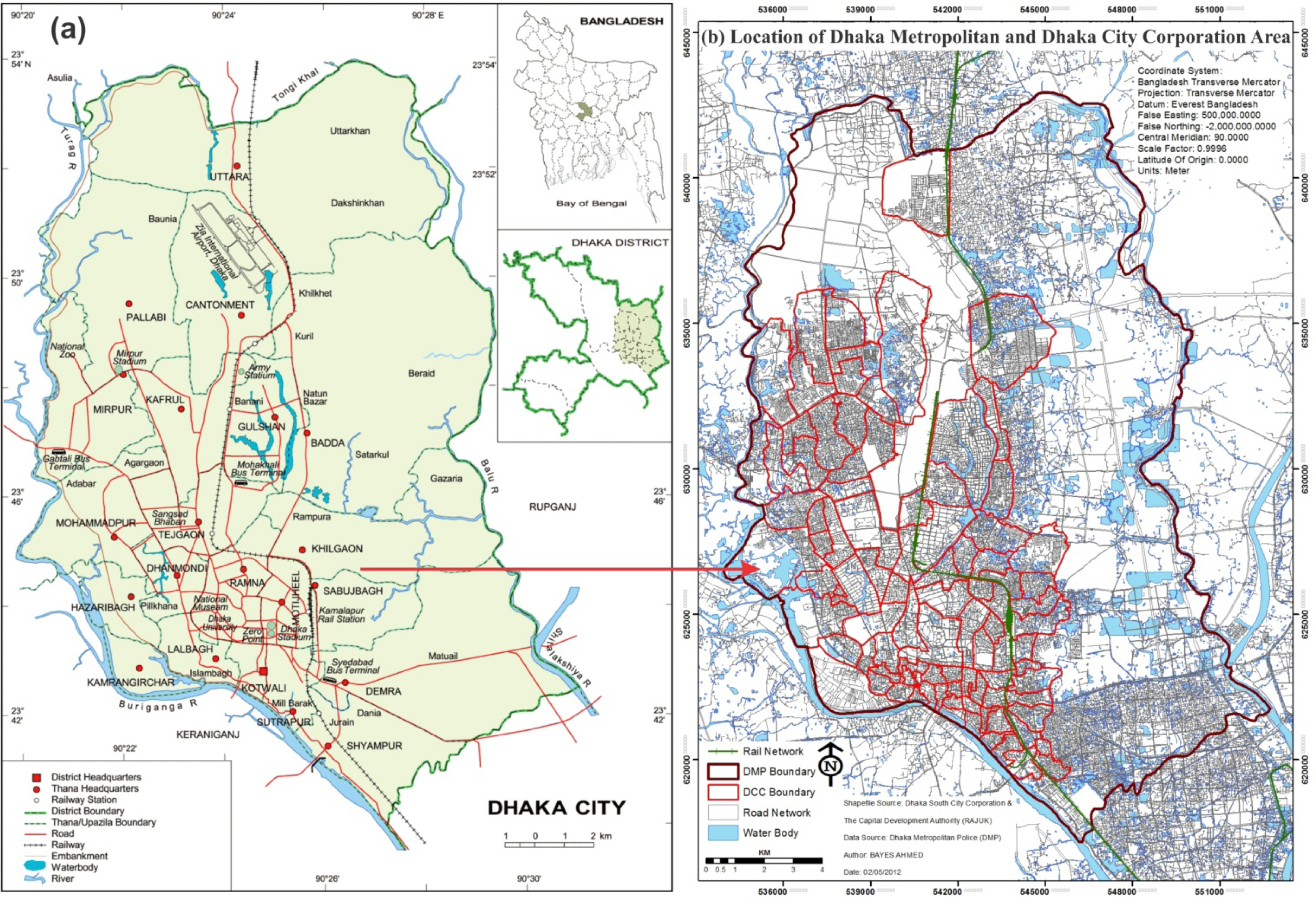
3.1. Case Study Area

This study was conducted in the context of Dhaka, Bangladesh. Dhaka, the capital of Bangladesh, is one of the fastest growing mega-cities of the world [20]. Therefore, although it is likely that such rapid urbanization in Dhaka has a major impact on land cover changes and consequently on the urban micro-climate, little is known about these trends so far in this context. The study area for this research covers the extent of Dhaka Metropolitan (DMP) area (Figure 1).
Dhaka is one of the largest urban agglomerations and the most densely populated mega city in the world. It is the home of more than 16 million people with a total land area of approximately 304.16 km2. The population of this city has increased by approximately 11 million in the past two decades [20]. Due to this population explosion mainly due to rural-urban migration and partially due to natural growth, Dhaka is expanding both vertically and horizontally. As discussed earlier, these expansions have been identified to be the major contributors of LST increase [20]. Existing evidences to date also justify the above argument because an upward shift of temperature has been noted in the last five decades, with an abrupt fluctuation in the minimum and maximum temperature levels (Figure 2).

3.2. Data Collection

Landsat satellite images (1989, 1999, and 2009) were downloaded from the official website of US Geological Survey (USGS) and used in order to reach the research objectives [55] (see Table 1 for details). The study area is located in the Landsat path 137 and row 44. The Universal Transverse Mercator (UTM) projection (within Zone 46 North) and the World Geodetic System (WGS)—1984 datum were applied to the images. The pixel sizes of the images were 30 × 30 m. Note that the three images were captured in different time periods; as a result, the atmospheric conditions might be different. However, the images were processed to level-one terrain-corrected (L1T) product. L1T provides systematic radiometric and geometric accuracy by incorporating ground control points while employing a Digital Elevation Model (DEM) for topographic accuracy. Geodetic accuracy of the product depends on the accuracy of the ground control points and the resolution of the DEM used [55].
In addition to the satellite images, a number of land use maps of the study area were collected in order to verify the accuracy of the classified images. The land use maps represented different time periods (e.g., 1987, 2001 and 2010). The maps were collected from the Survey of Bangladesh, which is a national organization responsible for surveying and preparing map products in the country. Therefore, the maps are generally consistent in terms of scale, units, and methods. However, while the existing maps can be valuable qualitative tools, they can result in the error matrix expressing merely differences between the reference data and the map data classification schemes, rather than map error. The scales of the maps were 1:20,000 including the classes- roads, railways, service, hydrography, boundary, cultivated area, low land, village, residential area, under development area, market/commercial area, educational area, industrial area, park and play ground; airport, graveyard, river, and lake.

4. Methods

The primary objective of this research is to model/simulate future LST. This was done through simulating future land cover changes, because empirical evidence has shown that a strong relationship exists between land cover indices (e.g., NDVI) and LST, as discussed in Section 2.3. Land cover maps of the DMP area were simulated for the period of 2019 and 2029, based on the patterns of land cover changes from 1989 to 2009. Four land cover indices were derived from the simulated land cover for each period including: NDVI, NDWI, NDBI, and NDBaI. The following sub-sections briefly present each of these steps.

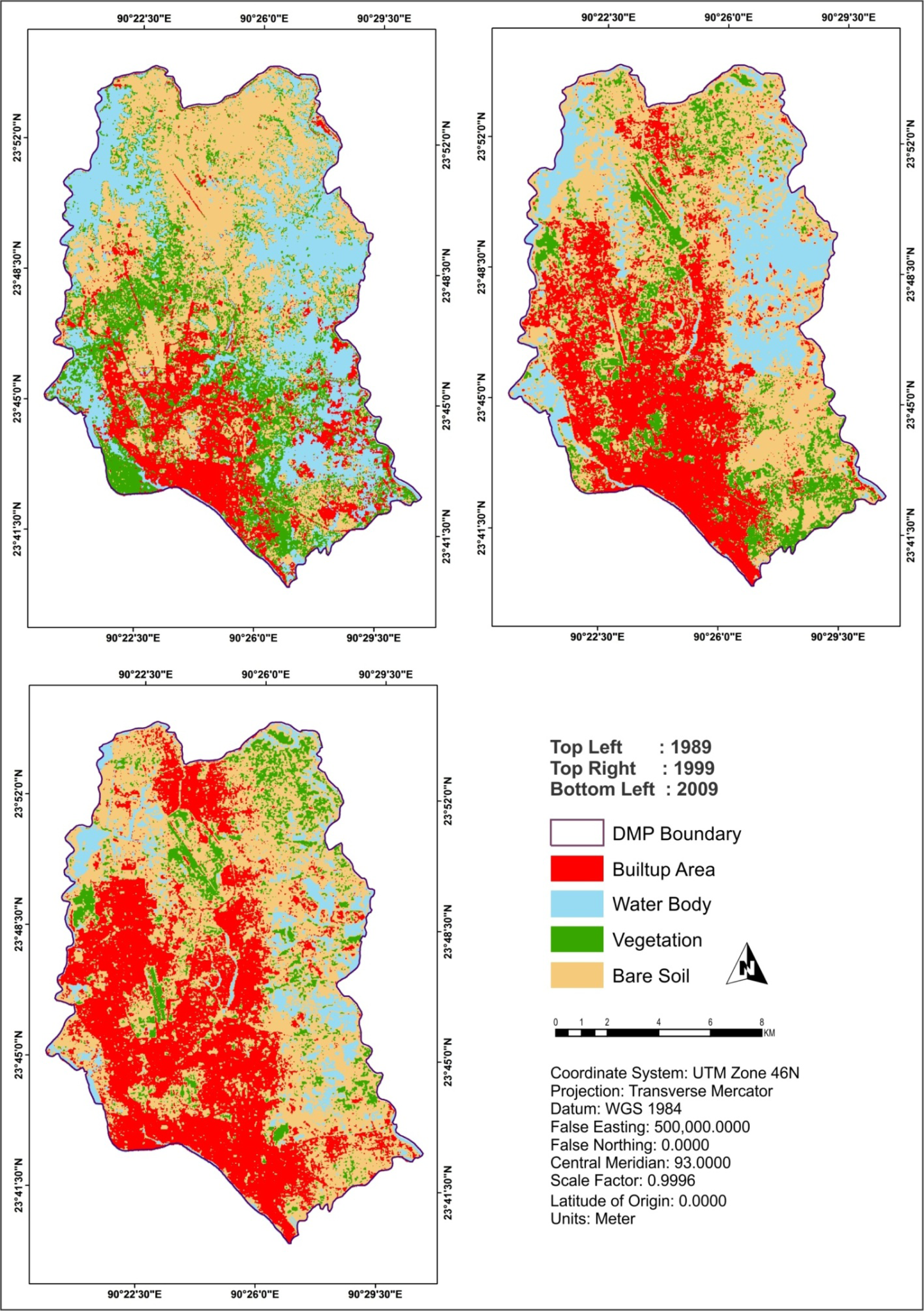
4.1. Derivation of Land Cover Maps

The acquired satellite images (1989, 1999, and 2009) were classified into four broad land cover types, as shown in Table 2. A supervised classification method was applied as it relies on a priori knowledge of the study area. All the images were analyzed with respect to their spectral and spatial profiles in order to develop training sites [20]. A chosen color composite (RGB = 432) was used for digitizing polygons around each training site for similar land cover. Then a unique identifier was assigned to each known land cover type [52]. The training sites developed for this research were based on the reference data and ancillary information collected from various sources.
When the digitization of the training sites was completed, the statistical characterizations (i.e., signatures) of each land cover class were developed [20]. Then, a maximum likelihood classification method was used with equal priori-probability for all classes. The maximum likelihood classifier calculated for each class the probability of the cell belonging to that class given its attribute values [30]. Consequently, a filtering technique was applied to generalize the classified land cover images. This post-processing operation replaced the isolated pixels to the most common neighboring class [52]. Finally, the generalized images were reclassified to produce the final version of land cover maps for different years (Figure 3).
The classified images were then assessed for accuracy based on a random selection of 200 reference pixels for each time period, which were compared against the collected land use maps [52]. The overall accuracies of the classified images (1989, 1999, and 2009) were, respectively, found to be 86.48%, 90.69%, and 94.83%, with Kappa coefficients of 0.86, 0.91, and 0.95 (Table 3). Note that the Kappa coefficient is a measure of the proportional (or percentage) improvement by the classifier over a purely random assignment to classes [56,57]. On the other hand, the user’s accuracy measures the proportion of each land cover class, which is correct whereas producer’s accuracy measures the proportion of the land base, which is correctly classified. It is observed that the accuracy of the land cover images is increasing over time. The reason is the availability of more detailed and higher resolution reference maps in recent times.

4.2. Retrieval of Land Surface Temperature

Surface radiant temperature is derived from geometrically corrected TM and ETM+ thermal infrared (TIR) channel (band 6). Band 6 records the radiation with spectral range in 10.4–12.5 μm from the surface of the earth [55]. The geometrically rectified images are free from distortions related to the sensor (e.g., jitter, view angle effects), satellite (e.g., attitude deviations from nominal), and Earth (e.g., rotation, curvature, relief) [55].
Although the impact of the diurnal heating cycle on the LSTs will be an interesting issue to address, there has been no attempt to include it here because TM/ETM+ images do not provide day and night infrared images at the same day. This is why the variability of LST at overpass time in different years is not analyzed. Moreover, because absolute temperatures are not used for the purpose of computation, atmospheric correction was not carried out at this stage. It means no radiometric normalization has been performed. These can be considered as some potential limitations of this research.
The LST was measured from the individual thermal images and were compared between different time periods. Based on the literature, different retrieval methods of brightness temperature from the TM and ETM+ images were applied as discussed below [5].

4.2.1. Retrieval of LST from the Landsat 5 TM Images

Based on Chen et al. (2002), a two step process was followed to derive brightness temperature from the Landsat 5 TM Images in this research [58]. In the first step, the digital numbers (DNs) of band 6 were converted to radiation luminance (RTM6) using the following formula:
R TM 6 = V 255 ( R max R min ) + R min
where, V represents the DN of band 6, and
R max = 1.896 ( mW × cm 2 × sr 1 )
R min = 0.1534 ( mW × cm 2 × sr 1 )
In the second step, the radiation luminance was converted to at-satellite brightness temperature in Kelvin, T(K), using the following equation:
T = K 1 ln ( K 2 / ( R TM 6 / b ) + 1 )
where, K1 = 1260.56 K and K2 = 607.66 (mW × cm−2 × sr−1 μm−1), which are pre-launch calibration constants under an assumption of unity emissivity; b represents effective spectral range, when the sensor’s response is much more than 50%, b = 1.239(μm) [55].

4.2.2. Retrieval of LST from the Landsat 7 ETM+ Images

In this research, a two step process was also used to retrieve brightness temperature from the Landsat 7 ETM+ images based on the literature [5,55]. In the first step, the DNs of band 6 were converted to radiance based on the following formula
Radiance = LMAX LMIN QCALMAX QCALMIN × ( QCAL QCALMIN ) + LMIN
where, information can be obtained from the header file of the images, QCALMIN = 1, QCALMAX = 255, QCAL = DN, and LMAX and LMIN (also given in the header file of the images) are the spectral radiances for band 6 at digital numbers 1 and 255 (i.e., QCALMIN and QCALMAX), respectively [55].
In the second step the effective at-satellite temperature of the viewed Earth-atmosphere system, under the assumption of a uniform emissivity, could be obtained by the following equation:
T = K 2 ln ( K 1 / L λ + 1 )
where, T is the effective at-satellite brightness temperature in Kelvin; K1 = 666.09 (watts/(meter2 × ster × μm)) and K2 = 1282.71 (Kelvin) are calibration constants; and Lλ is the spectral radiance in watts/(meter2 × ster × μm) [55].

4.3. Classification of the Heat Zones

The temperature values derived in ‘Kelvin (A)’ from the above two processes were converted in to ‘Degree Celsius (B)’ using the following equation:
B = A 273.15
This research found that the temperature values ranged from 15 °C to 36 °C, which were subsequently categorized into six classes (<18 °C, 18 °C to <21 °C, 21 °C to <24 °C, 24 °C to <27 °C, 27 °C to <30 °C, and ≥30 °C) (see, Figure 4).

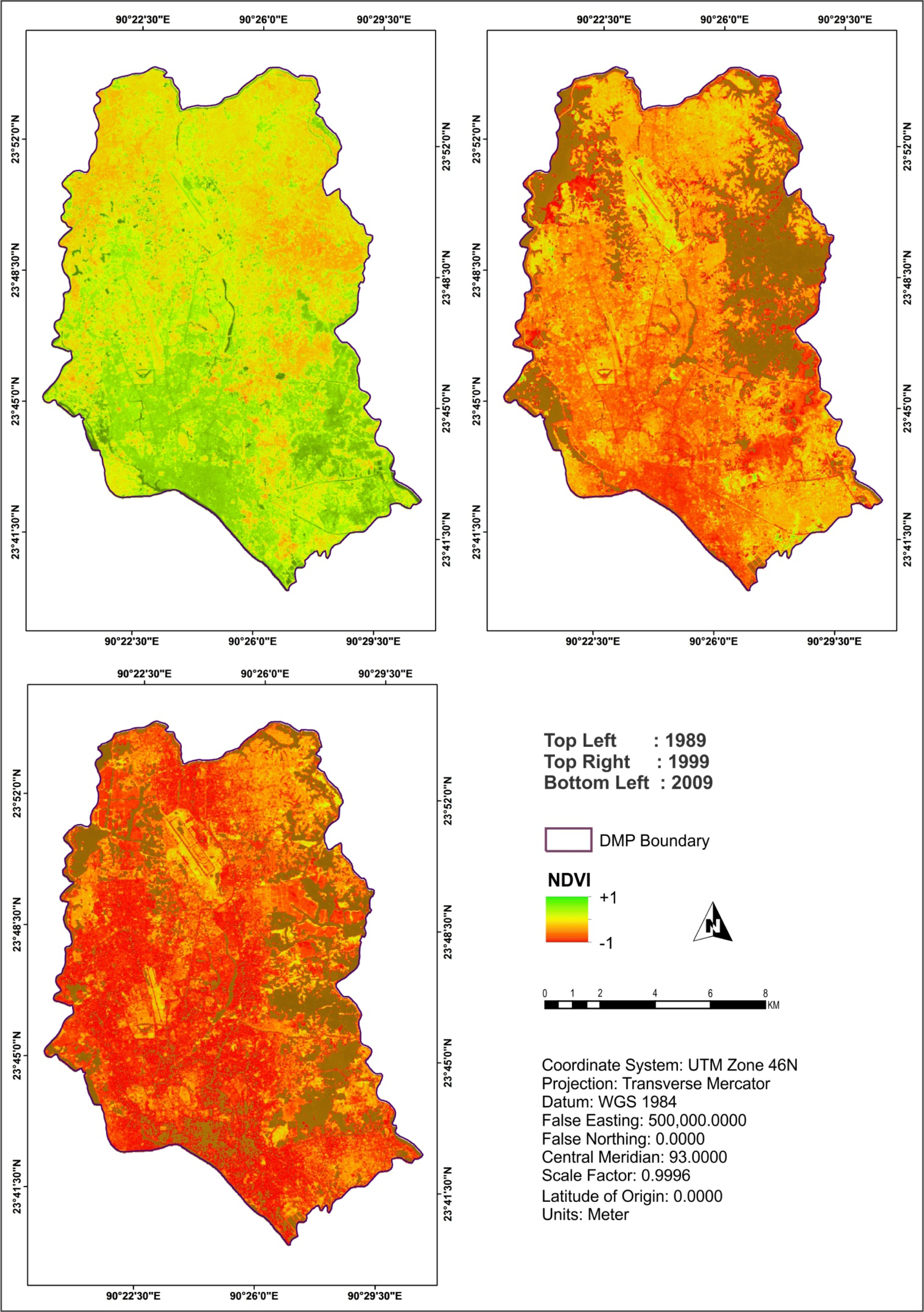
4.4. Derivation of NDVI, NDWI, NDBI, and NDBaI from the Landsat Imagery

As indicated earlier, four land cover indices were derived in this research including NDVI, NDWI, NDBI, and NDBaI. The following formulas, from the literature, were used to derive their scores [5]:
NDVI = b 4 b 3 b 4 + b 3
NDWI = b 4 b 5 b 4 + b 5
NDBI = b 5 b 4 b 5 + b 4
NDBaI = b 5 b 6 b 5 + b 6
where b3, b4, b5 and b6 are the DN values of each pixel in the Landsat TM/ETM+ visible red band 3 (0.63–0.69 μm), near-infrared band 4 (0.76–0.90 μm), middle infrared band 5 (1.55–1.75 μm), and thermal infrared band 6 (10.4–12.5 μm), respectively [55]. The NDVI map is illustrated in Figure 5.

4.5. Simulating Land Cover Maps for 2019 and 2029

As discussed earlier, there are many land use/cover change modeling techniques available (see Section 2.4). The choice of a right simulation technique/model depends upon individual context (e.g., the processes of land transformation), availability of datasets, objective of the research, and the accuracy of the prediction [20,51]. In this research, the combination of Markov Chain [59] and MLP modeling techniques [60] were applied to project the future land cover patterns due to their accuracy in outcomes and wide acceptability [61,62]. The MLP neural network model takes into account the rate of changes (e.g., expansion) in the built-up areas at the expense of other land cover types (e.g., in this case water body, vegetation, and bare soil). A great advantage of using this model is that it gives the opportunity to model several or even all the transitions at once. A description on the MLP Markov modeling technique can be found in Ahmed and Ahmed (2012), and as a result, is not described here in detail [52].
As the driving force (change to built-up area) for all these transitions are the same here, therefore it is possible to create a common group of explanatory variables that can adequately model all the transitions [20]. First, the observed land cover changes (the transitions from other land cover types to built-up areas) were used as the dependent variables; whereas the spatial variables (distance from all land cover types to built-up areas, water body, vegetation, and bare soil; the empirical likelihood transformation) were used as the independent variables. These two types of variables were used to train the MLP Markov model and to produce the transition potential maps. In this case, the MLP running statistics, based on the training and testing root mean square curves, gives an accuracy rate of 90.8%, which is considered to be good for this type of analysis [52,56]. The potential maps depict, for each location, the potential it has for each of the modeled transitions. Second, land cover conversions were predicted using the Multi-Objective Land Allocation (MOLA) algorithm [63]. The MOLA looks through all conversions to list the host classes that lose some amount of land and the receiver classes that acquire some amount of land from each host [64]. The quantities of conversions were determined by the Markovian conversion probabilities [65]. After this, a multi-objective allocation was run to allocate land for all receivers of a host class [63,64]. The results of the reallocation of each host class were then overlaid to produce the final predicted maps [20,52].

4.6. Simulating LST for 2019 and 2029

A three step method was applied in order to simulate LST for 2019 and 2029, as described in this section. Initially, a correlation (bivariate) analysis was conducted between each land cover index (e.g., NDVI) and the LST for each of the time periods (1989, 1999, and 2009) in order to explore the relationships over the periods. The analysis showed that the bivariate correlations are statistically significant and hold over the years. Second, given that the bivariate correlations were significant, a multiple regression analysis using the derived LST for 2009 as the dependent variable and the four land cover indices (NDVI, NDBI, NDWI, and NDBal) for 2009 as independent variable was warranted in order derive a regression equation to be used for projecting the future indices (2019 and 2029). However, a correlation analysis between the indices (e.g., between NDVI and NDBI) showed that the indices were significantly correlated with each other. As a result, the regression analysis was conducted only based on the NDVI in order to avoid the multicollinearity effect from the regression model. The model estimated a constant and a coefficient showing how the NDVI is related with the LST. Third, given that the explanatory power of the model was found to be representative of previous studies on this topic (i.e., explained more than 95% variance in data), the NDVI was, therefore, used to simulate LST for 2019 and 2029. To do this, the NDVI was simulated first for 2019 and 2029 using the Stochastic Markov model [52].
In general, in Markovian processes the future state of a system in time t2 can be modeled/predicted based on the immediate preceding state; time t1. Therefore, the future state can be predicted not based on the past but rather the present [20,47]. Initially the NDVI images were reclassified into suitable classes for Markov chain analysis. It produces a transition matrix, a transition areas matrix and a set of conditional probability images by analyzing two qualitative NDVI images from two different dates (1999 and 2009). Each conditional probability image shows the possibility of transitioning to another class [20,52]. The next step is to make one single NDVI map for future prediction aggregating all the Markovian conditional probability images. The final predicted land cover map of 2019 will be based on the past ten year’s land cover change pattern on the basis of Markov chain analysis. This prediction is performed by a Stochastic Choice decision model [20]. Stochastic Choice creates a stochastic NDVI map by evaluating and aggregating the conditional probabilities in which each class can exist at each pixel location against a rectilinear random distribution of probabilities [54]. This is how the NVDI maps of 2019 and 2029 were simulated. Finally the simulated NDVI images were used to produce the LST maps of 2019 and 2029 respectively using the regression equation.

5. Results

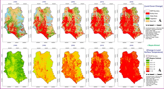
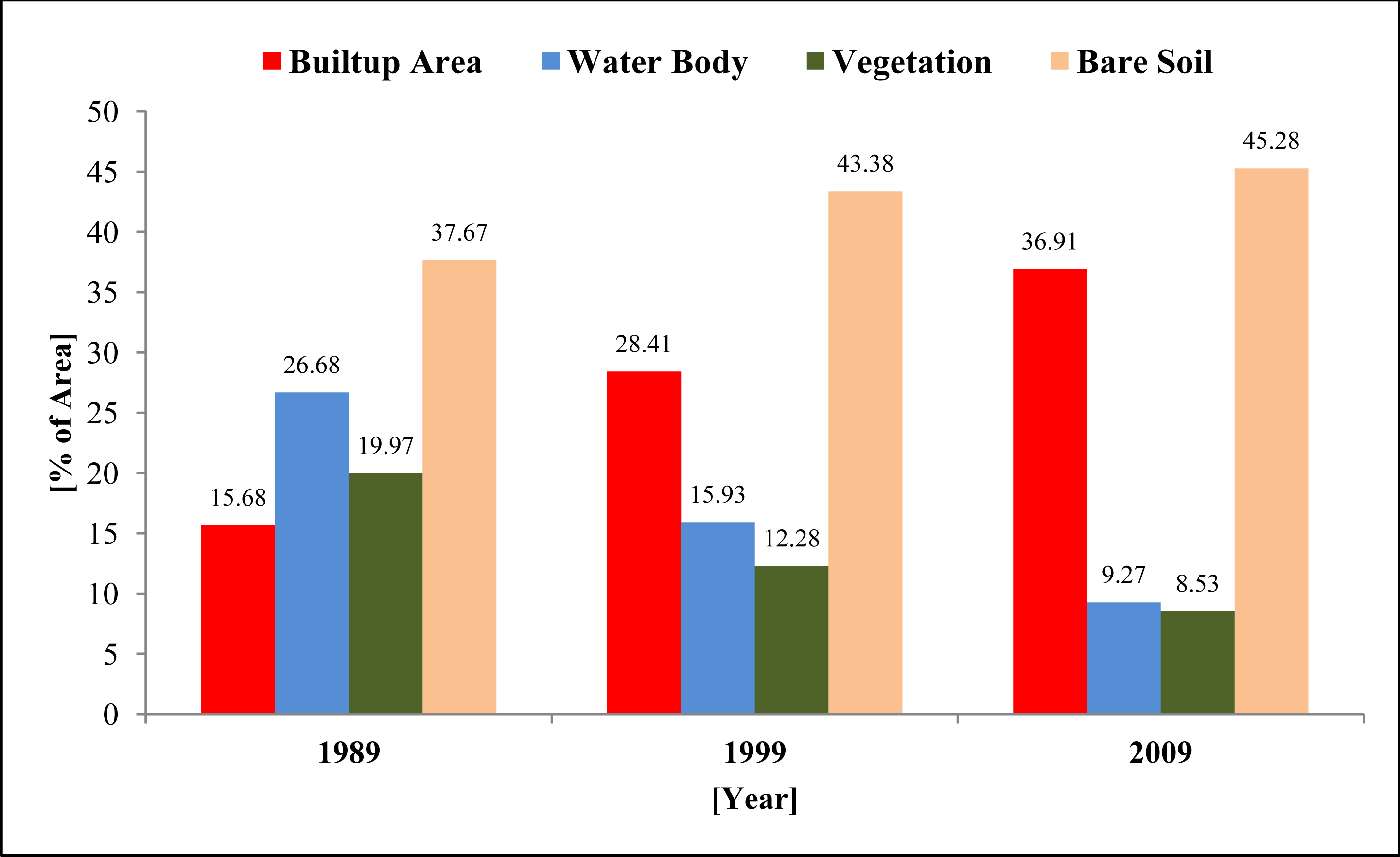
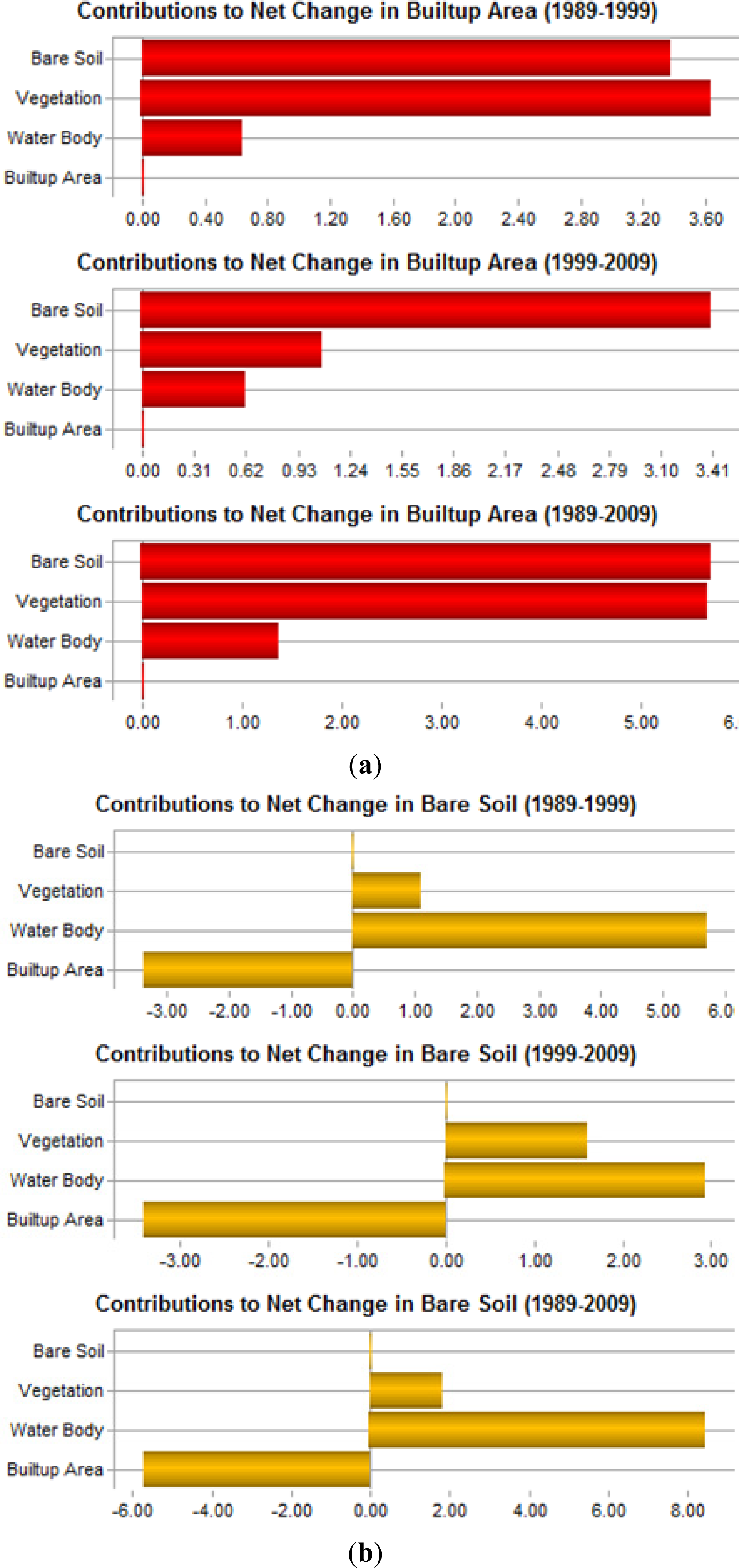
5.1. Patterns of Land Cover Changes

Figure 6 shows the distribution of land cover in the DMP area for the three time periods considered in this research. Two trends are clearly distinguishable from the figure: (a) built-up area and bare soil increased gradually over the periods; and (b) water body and vegetation declined gradually. More specifically built-up area increased by 88.78% in the past 20 years, from 1989 to 2009. However, two things are not explainable from Figure 6. First, it is unclear whether the built-up areas were only the receiver of lands from other types or donors as well to other types (e.g., converted from built-up to water body). Second, the patterns of conversions like the extent of conversion from one category to the others). In order to understand these relationships, further analyses were conducted (Figures 7 and 8).
Figure 7 illustrates that there was a slight loss in built-up area category in both time periods (e.g., 1989–1999, and 1999–2009). This means that some parts of the previously existed built-up areas were converted into some other land cover classes. However, a substantial change occurred in the bare soil category in both periods. This land cover category both gained and lost lands with almost an equal amount in each period (Figure 7). Figure 8 illustrates the conversion patterns between the categories. It shows that bare soil was the main contributor to forming the built-up areas followed by vegetation and water body (Figure 8a). In contrast, only water body and vegetation were converted into bare soil. Built-up area was not converted into bare soil type at all (Figure 8b).

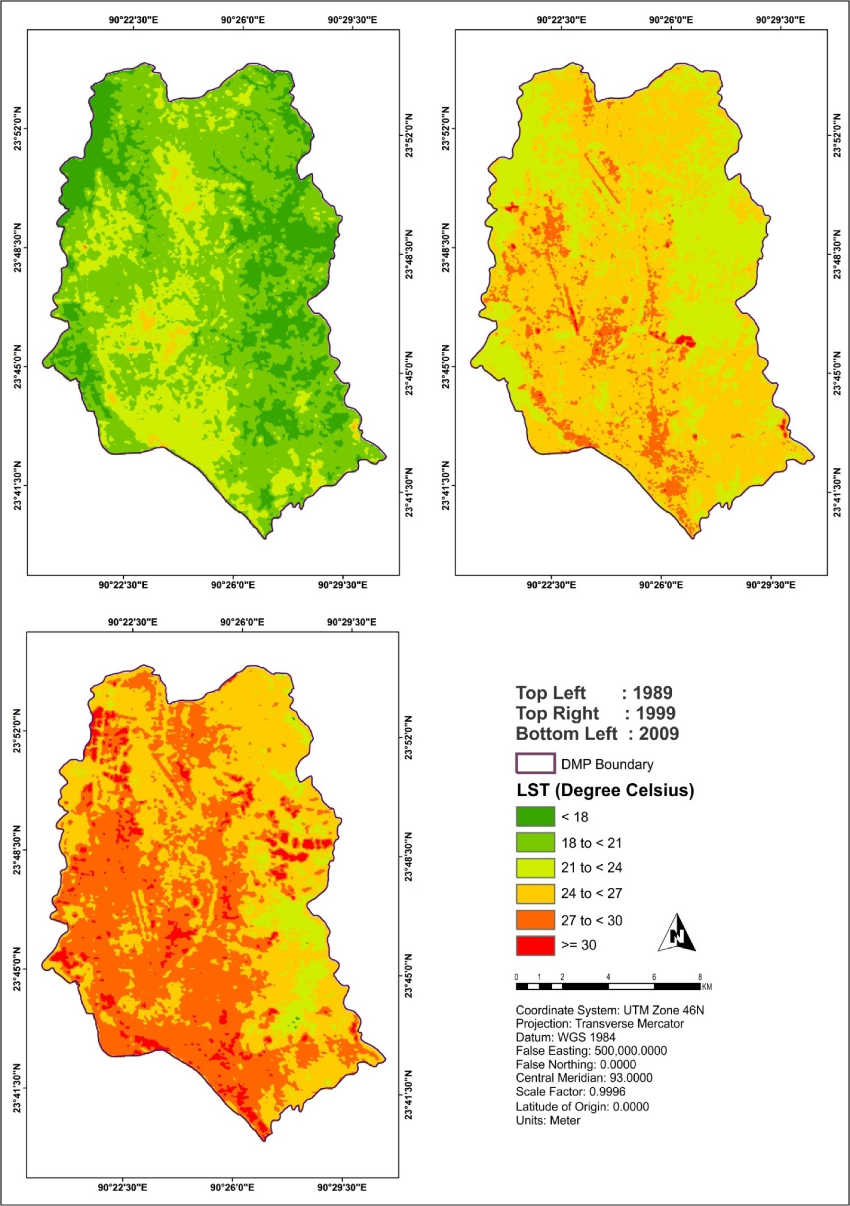
5.2. Change in Land Surface Temperature

Figure 4 shows the patterns of LST changes in the three time periods (1989, 1999, and 2009). The results show that the LSTs ranged from 15.44 °C to 28.12 °C, 18.39 °C to 34.22 °C and 23.03 °C to 35.73 °C.
Figure 9 shows that no areas in DMP experienced a temperature of ≥ 30 °C in 1989. Around 0.35% areas of the DMP experienced this temperature level in 1999, which was found to increase to around 5% in 2009. In 1989, a larger part of the DMP area (74%) fell within the lower temperature zones (<18 °C to < 21 °C) (Figure 9). But in 1999, a majority of the area (91.40%) was found to fall into the mid-temperature zones (21 °C to < 27 °C). This trend continues, and a larger portion of the DMP area (44%) moved into the higher temperature zones (27 °C to <30 °C) in 2009. Another noticeable fact is that no area remained in the lower heat zones in 2009 (Figure 9).

5.3. Temperature Variations for Different Land Cover Types

Weng (2001) has highlighted that the best way to understand the impact of land cover changes on LST is to investigate the links between the thermal signatures and land cover types [36]. Figure 10 summarises the average LST values by land cover type in the three periods. Clearly, the built-up land exhibited the highest LST, followed by bare soil, water body, and vegetation in all three periods. These findings are similar to that reported by Weng (2001), and Weng and Yang (2004) [36,39]. The findings signify that built-up areas increase surface temperature by replacing natural vegetation with non-evaporating, non-transpiring surfaces.
In addition, noticeable from Figure 10 is that the LST increased for all land cover types over the periods (e.g., even for vegetation); again suggesting the urban warming effect—otherwise temperature would have not been increased for vegetation. Ren, et al. also reported similar urban micro-climate warming effect in China. Their study has shown that both rural and urban areas experienced a rapid temperature increase in the last two decades [66]. However, in comparison with their rate of temperature increase (e.g., 0.32 °C/10 year), the rate of increase in the DMP was higher as shown in Figure 10. This is probably due to the fact that the DMP area experienced a rapid growth. On the other hand, the differences in the temporal resolution of the images might have an impact on this result. However, the results are indicative enough to support the urban area-warming phenomenon in the DMP area.

5.4. Relationship between Temperature and Land Cover Indices

Four land cover indices (e.g., NDVI, NDWI, NDBI, and NDBaI) were derived in order to establish quantifiable relationships between LST and the indices. As documented in the literature, a higher level of LST was found to be associated with a lower NDVI in this research (Figures 4 and 5). Figure 11a presents the relationship between LST and NDVI. In 1989, the NDVI ranged between −0.17 and +0.70, which gradually reduced to between −0.72 and +0.29, in 2009. Therefore, it can be said that the NDVI decreased in DMP over time (Figure 5).
This research also found that the NDWI and NDBaI values decreased over the periods as well suggesting that both the water content in vegetation and bareness of soil also declined. Figures 11 and 12 show, the correlations and linear regression equations of the LST and the different indices from 1989 to 2009. The results of multiple correlation and regression analyses indicate that LST presents a positive correlation with NDBI (Figure 12a) and negative correlations with NDVI, NDWI, and NDBaI (Figures 11a,b and 12b).

5.5. Simulating the Future Land Cover Dynamics

The main objective of this research was to simulate the future LST in the DMP area. In order to reach the objective, the future land covers of the area were simulated first. As mentioned earlier, the MLP Markov Chain model was used to simulate land cover for 2019 and 2029. The simulated land cover maps are shown in Figure 13. Note that 37% of the DMP area was categorized as built-up in 2009. The simulation results suggest that approximately 49% and 57% of the DMP area will be converted into “built-up area” land cover type in 2019 and 2029, respectively (Figure 13).

5.6. Simulating the Future LST Maps

The simulated LST maps of 2019 and 2029 are shown in Figure 14. It is found that approximately 56% and 87% areas of DMP will fall in the highest temperature zone (≥30 °C) in 2019 and 2029, respectively (Figure 14).

6. Discussion

This research models the impacts of land cover changes on land surface temperature (LST) in Dhaka Metropolitan (DMP) area for the period of 2019 and 2029. Numerous studies have investigated the impact of land cover changes on LST [7,11]. On the other hand, a handful literature exist that model urban growth for future [66,67]. This study is the first of its kind that attempted to combine both techniques and predicted LST based on simulated land cover changes. In addition to the simulated LST, this research also examined the observed relationship between land cover changes and LST in three time periods (1989, 1999, 2009) for the same area. The observed relationships were found to be consistent with the well-established findings in the literature that: (a) built-up areas exhibited the highest temperature, whereas the lowest temperature was found to be associated with the vegetated/forested areas within DMP area for all three periods [36]; (b) built-up areas increased significantly (89%) over the periods at the expense of vegetation, bare soil and water bodies [66], and as a result, more areas fell within the higher temperature zones over the periods; (c) a gradual increase in temperature was evident for all land cover types in DMP—suggesting the urban micro-climate warming effect in the area [68]; and (d) regression analysis resulted with a positive association between LST and NDBI; and a negative association between LST and other three land cover indices (e.g., NDVI, NDWI, and NDBaI) considered in this research [35,37].
Given that the findings from the observed relationships are consistent with the literature, it is believed that the simulated relationships are likely to be defendable because they are based on well-established methods in the literature- MLP Markov. The simulation results from the model were found to be a real concern for the policy makers of DMP area. The findings presented in this paper suggest that there would not be any spatially distributed sporadic UHI within the study area rather the whole DMP area would become an UHI in Bangladesh. Note that, urbanization is the main driver of land cover changes and consequently LST. However, unless undertaking a radical decentralization policy, it is difficult to stop or reverse the urbanization process in DMP because it contains all the major opportunities (e.g., job) and services (e.g., hospital/education) of the country [20]. Growth management policies (e.g., green belt) can be implemented that would contain the growth and consequently help reducing UHI effect [69]. In addition, policies must not be limited to horizontal growth management only. As discussed in Section 2.2, vertical growth (e.g., building height) can also cause LST. Additional consideration to implement the new urbanism (e.g., green building) concepts in the planning permission (or development assessment) stage of development would also help reducing the LST in the DMP area [70].
Despite the above findings are indicative, they should be read with caution because the results were derived from satellite images with different time periods. Further research should seek to validate the findings reported in this research using more authentic datasets. In addition, although the UHI and LST were often used interchangeably in this paper, they are not the identical concepts rather LST is considered to be just one contributing factor to UHI. The calculation of UHI requires data from a comparative geography (e.g., rural vs. urban), which was not considered in this research. Further research should seek to extend the study area by incorporating the rural/less urbanized surroundings of DMP area in order to simulate UHI effect in this context.

7. Conclusions

This is the first study, to the knowledge of the authors that demonstrated a method of deriving future land surface temperature (LST) of urban areas based on the simulation from observed relationships between land cover and LST changes in Dhaka Metropolitan (DMP) area. In doing so, the following conclusions were reached: (1) the amount of built-up area has doubled between 1989 and 2009, and is expected to increase three-fold and four-fold by 2019 and 2029, respectively; (2) a significant negative association between NDVI and LST where as a significant positive association between NDBI and LST exist which suggest that vegetation reduces the LST and built-up areas increases LST. Therefore, future city planning should focus more on urban greening; (3) more DMP areas are gradually shifting towards the highest temperature zone due to the expansion of built-up areas, and if the current trend continues then almost the entire DMP area will be an UHI in 2029. A compact-town like decentralization of urban areas (e.g., satellite-towns) is, therefore, a possible way forward in order to prevent the formation of large-scale urban heat island effect in the future, (4) the study used one land cover index (e.g., NDVI) and applied a simple regression equation for the derivation of future LST. It is possible that the different land cover indices can be used together as independent factors in a multiple regression equation model in order to derive the LST in a more robust way, possibly through undertaking a factor analysis. Future study should seek to incorporate these and improve upon the model presented here.

Acknowledgments

The authors would like to thank the Survey of Bangladesh, the Bangladesh Meteorological Department, the Capital Development Authority (RAJUK) and the US Geological Survey for assisting this research with datasets. The work was partially supported by the Korea Science and Engineering Foundation (KOSEF) grant funded by the Korean Government (MSIP) [No. 2010-0029446]. Finally we thank the three anonymous reviewers and the editors of ‘Remote Sensing’ journal for their constructive comments that improved the quality of this paper.

Conflicts of Interest

The authors declare no conflict of interest.

References

  1. He, F.; Liu, J.Y.; Zhuang, D.F.; Zhang, W.; Liu, M.L. Assessing the effect of land use-land cover change on the change of urban heat island intensity. J. Theor. Appl. Climatol 2007, 90, 217–226. [Google Scholar]
  2. Trenberth, K.E. Climatology (communication arising): Rural land-use change and climate. Nature 2004, 427, 213. [Google Scholar]
  3. Patz, J.A.; Lendrum, D.C.; Holloway, T; Foley, J.A. Impact of regional climate change on human health. Nature 2005, 438, 310–317. [Google Scholar]
  4. Kalnay, E.; Cai, M. Impact of urbanization and land-use change on climate. Nature 2003, 423, 528–531. [Google Scholar]
  5. Chen, X.-L.; Zhao, H.-M.; Li, P.-X.; Yin, Z.-Y. Remote sensing image-based analysis of the relationship between urban heat island and land use/cover changes. Remote Sens. Environ 2006, 104, 133–146. [Google Scholar]
  6. Lo, C.P.; Quattrochi, D.A. Land-use and land-cover change, urban heat island phenomenon, and health implications: A remote sensing approach. Photogramm. Eng. Remote Sens 2003, 69, 1053–1063. [Google Scholar]
  7. Deosthali, V. Impact of rapid urban growth on heat and moisture islands in Pune City, India. Atmos. Environ 2000, 34, 2745–2754. [Google Scholar]
  8. Mutizwa-Mangiza, N.D.; Arimah, B.C.; Jensen, I.; Yemeru, E.A.; Kinyanjui, M.K. Cities and Climate Change: Global Report on Human Settlements 2011, 1st ed; Earthscan Ltd: London, UK, 2011; pp. 1–12. [Google Scholar]
  9. Ye, H.; Wang, K.; Huang, S.; Chen, F.; Xiong, Y.; Zhao, X. Urbanisation effects on summer habitat comfort: A case study of three coastal cities in southeast China. Int. J. Sust. Dev. World 2010, 17, 317–323. [Google Scholar]
  10. Howard, L. The climate of London. London Harvey Dorton 1833, 2, 1818–1820. [Google Scholar]
  11. Liu, L.; Zhang, Y. Urban heat island analysis using the Landsat TM data and ASTER data: A Case study in Hong Kong. Remote Sens 2011, 3, 1535–1552. [Google Scholar]
  12. Streutker, D.R. A remote sensing study of the urban heat island of Houston, Texas. Int. J. Remote Sens 2002, 23, 2595–2608. [Google Scholar]
  13. Ohashi, Y.; Kida, H. Local circulations developed in the vicinity of both coastal and inland urban areas: A numerical study with a mesoscale atmospheric model. J. Appl. Meteor 2002, 41, 30–45. [Google Scholar]
  14. Souch, C.; Grimmond, S. Applied climatology: Urban climate. Prog. Phys. Geogr 2006, 30, 270–279. [Google Scholar]
  15. Jones, P.D.; Groisman, P.Y.; Coughlan, M.; Plummer, N.; Wang, W.; Karl, T.R. Assessment of urbanization effects in time series of surface air temperature over land. Nature 1990, 347, 169–172. [Google Scholar]
  16. Sheng, J.; Wilson, J.P.; Lee, S. Comparison of land surface temperature (LST) modeled with a spatially-distributed solar radiation model (SRAD) and remote sensing data. Environ. Model. Softw 2009, 24, 436–443. [Google Scholar]
  17. Weng, Q.; Lu, D. A sub-pixel analysis of urbanization effect on land surface temperature and its interplay with impervious surface and vegetation coverage in Indianapolis, United States. Int. J. Appl. Earth Obs. Geoinf 2008, 10, 68–83. [Google Scholar]
  18. Rosenzweig, C.; Karoly, D.; Vicarelli, M.; Neofotis, P.; Wu, Q.; Casassa, G.; Menzel, A.; Root, T.L.; Estrella, N.; Seguin, B.; et al. Attributing physical and biological impacts to anthropogenic climate change. Nature 2008, 453, 353–357. [Google Scholar]
  19. Oke, T.A. The Energetic Basis of the Urban Heat Island. Quart. J. Royal Meteor. Soc 1982, 108, 1–24. [Google Scholar]
  20. Ahmed, B. Urban land cover change detection analysis and modeling spatio-temporal Growth dynamics using Remote Sensing and GIS Techniques: A case study of Dhaka, Bangladesh. Erasmus Mundus Program, Universidade Nova de Lisboa (UNL), Instituto Superior de Estatística e Gestão de Informação (ISEGI), Lisbon, Portugal, 2011. [Google Scholar]
  21. Lowry, W.P. Empirical estimation of urban effects on climate: A problem analysis. J. Appl. Meteor 1977, 16, 129–135. [Google Scholar]
  22. Karl, T.R.; Diaz, H.F.; Kukla, G. Urbanization: Its detection and effect in the United States climate record. J. clim 1988, 1, 1099–1123. [Google Scholar]
  23. Gallo, K.P.; Tarpley, J.D. The comparison of vegetation index and surface temperature composites for urban heat-island analysis. Int. J. Remote Sens 1996, 17, 3071–3076. [Google Scholar]
  24. Streutker, D.R. Satellite-measured growth of the urban heat island of Houston, Texas. Remote Sens. Environ 2003, 85, 282–289. [Google Scholar]
  25. Fabrizi, R.; Bonafoni, S.; Biondi, R. Satellite and ground-based sensors for the urban heat island analysis in the City of Rome. Remote Sens 2010, 2, 1400–1415. [Google Scholar]
  26. Gallo, K.P.; Owen, T.W. Assessment of urban heat island: A multi-sensor perspective for the Dallas-Ft. Worth, USA region. Geocarto. Int 1998, 13, 35–41. [Google Scholar]
  27. Rinner, C.; Hussain, M. Toronto’s urban heat island- Exploring the relationship between land use and surface temperature. Remote Sens 2011, 3, 1251–1265. [Google Scholar]
  28. Xiong, Y.; Huang, S.; Chen, F.; Ye, H.; Wang, C.; Zhu, C. The impacts of rapid urbanization on the thermal environment: A remote sensing study of Guangzhou, South China. Remote Sens 2012, 4, 2033–2056. [Google Scholar]
  29. Essa, W.; Verbeiren, B.; van der Kwast, J.; van de Voorde, T.; Batelaan, O. Evaluation of the DisTrad thermal sharpening methodology for urban areas. Int. J. Appl. Earth Obs. Geoinf 2012, 19, 163–172. [Google Scholar]
  30. ArcGIS® 10 Help; Environmental Systems Research Institute: Redlands, CA, USA, 2012. Available online: http://help.arcgis.com/en/arcgisdesktop/10.0/help/ (accessed on 15 December 2012).
  31. Gao, B.C. NDWI—A normalized difference water index for remote sensing of vegetation liquid water from space. Remote Sens. Environ 1996, 58, 257–266. [Google Scholar]
  32. Maki, M.; Ishiahra, M.; Tamura, M. Estimation of leaf water status to monitor the risk of forest fires by using remotely sensed data. Remote Sens. Environ 2004, 90, 441–450. [Google Scholar]
  33. Zha, Y.; Gao, J.; Ni, S. Use of normalized difference built-up index in automatically mapping urban areas from TM imagery. Int. J. Remote Sens 2003, 24, 583–594. [Google Scholar]
  34. Zhao, H.M.; Chen, X.L. Use of normalized difference bareness index in quickly mapping bare areas from TM/ETM+. proceedings of 2005 IEEE International Geoscience and Remote Sensing Symposium, 2005. IGARSS’05, Seoul, Korea, 25–29 July 2005; pp. 1666–1668.
  35. Kalnay, E.; Cai, M. Impact of urbanization and land-use change on climate. Nature 2003, 423, 528–531. [Google Scholar]
  36. Weng, Q. A remote sensing-GIS evaluation of urban expansion and its impact on surface temperature in the Zhujiang Delta, China. Int. J. Remote Sens 2001, 22, 1999–2014. [Google Scholar]
  37. Weng, Q.; Lu, D.; Liang, B. Urban surface biophysical descriptors and land surface temperature variations. Photogram. Eng. Remote Sens 2006, 72, 1275–1286. [Google Scholar]
  38. Xiao, R.-B.; Ouyang, Z.-Y.; Zheng, H.; Li, W.-F.; Schienke, E.W.; Wang, X.-K. Spatial patterns of impervious surfaces and their impact on land surface temperature in Beijing, China. J. Environ. Sci 2007, 19, 250–256. [Google Scholar]
  39. Weng, Q.; Yang, S. Managing the adverse thermal effects of urban development in a densely populated Chinese city. J. Environ. Manag 2004, 70, 145–156. [Google Scholar]
  40. Pontius, R.G., Jr.; Spencer, J. Uncertainty in extrapolations of predictive land change models. Environ. Plan. B 2005, 32, 211–230. [Google Scholar]
  41. Silva, E.A.; Clarke, K.C. Calibration of the SLEUTH urban growth model for Lisbon and Porto, Portugal. Comput. Environ. Urban Syst 2002, 26, 525–552. [Google Scholar]
  42. Hilferink, M.; Rietveld, P. Land Use Scanner: An integrated GIS based model for long term projections of land use in urban and rural areas. J. Geogr. Syst 1999, 1, 155–177. [Google Scholar]
  43. Verburg, P.H.; de Nijs, T.C.M.; van Eck, J.R.; Visser, H.; de Jong, K. A method to analyse neighbourhood characteristics of land use patterns. Comput. Environ. Urban Syst 2004, 28, 667–690. [Google Scholar]
  44. Castella, J.C.; Boissau, S.; Trung, T.N.; Quang, D.D. Agrarian transition and lowland-upland interactions in mountain areas in northern Vietnam: Application of a multi-agent simulation model. Agric. Syst 2005, 86, 312–332. [Google Scholar]
  45. Pijanowski, B.C.; Gage, S.H.; Long, D.T. A Land Transformation Model: Integrating Policy, Socioeconomics and Environmental Drivers using a Geographic Information System. In Landscape Ecology: A Top down Approach; Harris, L., Sanderson, J., Eds.; CRC Press: Boca Raton, FL, USA, 2000; pp. 183–198. [Google Scholar]
  46. Kok, K.; Veldkamp, T.A. Evaluating impact of spatial scales on land use pattern analysis in Central America. Agric. Ecosyst. Environ 2001, 85, 205–221. [Google Scholar]
  47. Balzter, H. Markov chain models for vegetation dynamics. Ecolog. Model 2000, 126, 139–154. [Google Scholar]
  48. Santé, I.; García, A.M.; Miranda, D.; Crecente, R. Cellular automata models for the simulation of real-world urban processes: A review and analysis. Landsc. Urban Plan 2010, 96, 108–122. [Google Scholar]
  49. McConnell, W.; Sweeney, S.P.; Mulley, B. Physical and social access to land: Spatio-temporal patterns of agricultural expansion in Madagascar. Agric. Ecosyst. Environ 2004, 101, 171–184. [Google Scholar]
  50. Civco, D.L. Artificial neural networks for land-cover classification and mapping. Int. J. Geogr. Inf. Sci 1993, 7, 173–186. [Google Scholar]
  51. Pontius, R.G., Jr.; Boersma, W.; Castella, J.-C.; Clarke, K.; de Nijs, T.; Dietzel, C.; Duan, Z.; Fotsing, E.; Goldstein, N.; Kok, K.; et al. Comparing the input, output, and validation maps for several models of land change. Ann. Reg. Sci 2008, 42, 11–47. [Google Scholar]
  52. Ahmed, B.; Ahmed, R. Modeling urban land cover growth dynamics using multi-temporal satellite images: A case study of Dhaka, Bangladesh. ISPRS Int. J. Geo-Inf 2012, 1, 3–31. [Google Scholar]
  53. Atkinson, P.M.; Tatnall, A.R.L. Introduction Neural networks in remote sensing. Int. J. Remote Sens 1997, 18, 699–709. [Google Scholar]
  54. Eastman, J.R. IDRISI Selva Tutorial; Clark University; Worcester, MA, USA, 2012; pp. 267–275. [Google Scholar]
  55. Landsat 7 Science Data Users Handbook, 2010; National Aeronautics and Space Administration,; pp. 117–120. Landsat Project Science Office at NASA’s Goddard Space Flight Center: Greenbelt, MD, USA, 2010.
  56. Ahmed, B.; Ahmed, R.; Zhu, X. Evaluation of model validation techniques in land cover dynamics. ISPRS Int. J. Geo-Inf 2013, 2, 577–597. [Google Scholar]
  57. Cohen, J. A coefficient of agreement for nominal scales. Educ. Psychol. Meas 1960, 20, 37–46. [Google Scholar]
  58. Chen, Y; Wang, J.; Li, X. A study on urban thermal field in summer based on satellite remote sensing. Remote Sens. Land Resour 2002, 4, 55–59. [Google Scholar]
  59. Basharin, G.P.; Langville, A.N.; Naumov, V.A. The life and work of A.A. Markov. Linear Algebra Appl 2004, 386, 3–26. [Google Scholar]
  60. Atkinson, P.M.; Tatnall, A.R.L. Introduction Neural networks in remote sensing. Int. J. Remote Sens 1997, 18, 699–709. [Google Scholar]
  61. Pijanowski, B.C.; Brown, D.G.; Manik, G.; Shellito, B. Using neural nets and GIS to forecast land use changes: A land transformation model. Comput. Environ. Urban Syst 2002, 26, 553–575. [Google Scholar]
  62. Pijanowski, B.C.; Pithadia, S.; Shellito, B.A.; Alexandridis, K. Calibrating a neural network-based urban change model for two metropolitan areas of the Upper Midwest of the United States. Int. J. Geogr. Inf. Sci 2005, 19, 197–215. [Google Scholar]
  63. Khoi, D.D.; Murayama, Y. Forecasting areas vulnerable to forest conversion in the Tam Dao National Park Region, Vietnam. Remote Sens 2010, 2, 1249–1272. [Google Scholar]
  64. Eastman, J.R. IDRISI Selva Manual; Clark University: Worcester, MA, USA, 2012. [Google Scholar]
  65. Eastman, J.R.; Jin, W.; Kyem, P.A.K.; Toledano, R. Raster procedures for multi-criteria/multi-objective decisions. Photogramm. Eng. Remote Sens 1995, 61, 539–547. [Google Scholar]
  66. Tewolde, M.G.; Cabral, P. Urban sprawl analysis and modeling in Asmara, Eritrea. Remote Sens 2011, 3, 2148–2165. [Google Scholar]
  67. Zeug, G.; Eckert, S. Population growth and its expression in spatial built-up patterns: The Sana’a, Yemen case study. Remote Sens 2010, 2, 1014–1034. [Google Scholar]
  68. Ren, G.Y.; Chu, Z.Y.; Chen, Z.H.; Ren, Y.Y. Implications of temporal change in urban heat island intensity observed at Beijing and Wuhan stations. Geophys. Res. Lett 2007, 34, L05711. [Google Scholar]
  69. Park, H.-S. Features of the heat island in Seoul and its surrounding cities. Atmos. Environ 1986, 20, 1859–1866. [Google Scholar]
  70. Kibert, C.J. Sustainable Construction: Green Building Design and Delivery, 3rd ed; John Wiley and Sons, Inc: Hoboken, NJ, USA, 2012; p. 236. [Google Scholar]
Figure 1. Location of Dhaka Metropolitan (DMP) area (a) in Bangladesh and (b) in Dhaka City Corporation (DCC). Source: (a) Banglapedia, National Encyclopedia of Bangladesh, 2012, and (b) The Capital Development Authority (RAJUK), Dhaka, 2012.
Remotesensing 05 05969f1
Figure 2. Annual mean temperature (minimum and maximum) of Dhaka City (1960–2010). Date source: Bangladesh Meteorological Department, 2012.
Remotesensing 05 05969f2
Figure 3. Land cover maps of DMP area.
Remotesensing 05 05969f3
Figure 4. Spatial distribution of land surface temperature (LST).
Remotesensing 05 05969f4
Figure 5. NDVI distributions in DMP area (1989–2009).
Remotesensing 05 05969f5
Figure 6. Percentages of presence of land cover types in DMP area.
Remotesensing 05 05969f6
Figure 7. Gains and losses of the land cover types (Unit: % of Area).
Remotesensing 05 05969f7
Figure 8. Contributions to net change (a) in built-up area and (b) in bare soil of DMP area (Unit: % of Area).
Remotesensing 05 05969f8
Figure 9. Changing pattern of heat zones in DMP area.
Remotesensing 05 05969f9
Figure 10. The variations of mean LST over different land cover types.
Remotesensing 05 05969f10
Figure 11. (a) Correlation between NDVI and LST; (b) Correlation between NDWI and LST.
Remotesensing 05 05969f11
Figure 12. (a) Correlation between NDBI and LST; (b) Correlation between NDBaI and LST.
Remotesensing 05 05969f12
Figure 13. MLP Markov model simulated land cover maps of DMP area (2019 and 2029).
Remotesensing 05 05969f13
Figure 14. The simulated LST maps of DMP area (2019 and 2029).
Remotesensing 05 05969f14
Table 1. Details of Landsat satellite images. Source: US Geological Survey, 2012.
Respective YearDate Acquired (Day/Month/Year)Sensor
198913/02/1989Landsat 4–5 Thematic Mapper (TM)
199924/11/1999Landsat 7 Enhanced Thematic Mapper Plus (ETM+)
200926/10/2009Landsat 4–5 Thematic Mapper (TM)
Table 2. Details of the land cover types.
Land Cover TypeDescription
Built-up AreaAll infrastructure—residential, commercial, mixed use and industrial areas, villages, settlements, road network, pavements, and man-made structures.
Water BodyRiver, permanent open water, lakes, ponds, canals, permanent/seasonal wetlands, low-lying areas, marshy land, and swamps.
VegetationTrees, natural vegetation, mixed forest, gardens, parks and playgrounds, grassland, vegetated lands, agricultural lands, and crop fields.
Bare SoilFallow land, earth and sand land in-fillings, construction sites, developed land, excavation sites, open space, bare soils, and the remaining land cover types.
Table 3. Accuracy assessments of the land cover types.
YearUser’s Accuracy (%)
Producer’s Accuracy (%)
Overall Accuracy (%)Kappa Coefficient
Built-up AreaWater BodyVegetationBare SoilBuilt-up AreaWater BodyVegetationBare Soil
198987.2486.7185.6486.2285.6786.3986.0585.8886.480.86
199991.4288.5589.7890.4389.1390.6888.7290.3990.690.91
200993.5194.7793.6194.8394.7595.4493.5892.8694.130.95

