Combined Spatial and Temporal Effects of Environmental Controls on Long-Term Monthly NDVI in the Southern Africa Savanna


Abstract
:1. Introduction
2. Methods
2.1. Study Area
2.2. Remote Sensing and Climate Data
2.2.1. NDVI
2.2.2. Climate Data
2.3. Conceptual Basis for Analysis
2.4. Dynamic Factor Analysis (DFA)
2.4.1. Dimension Reduction of Candidate Explanatory Variables
2.4.2. NDVI Analysis Procedure
3. Results
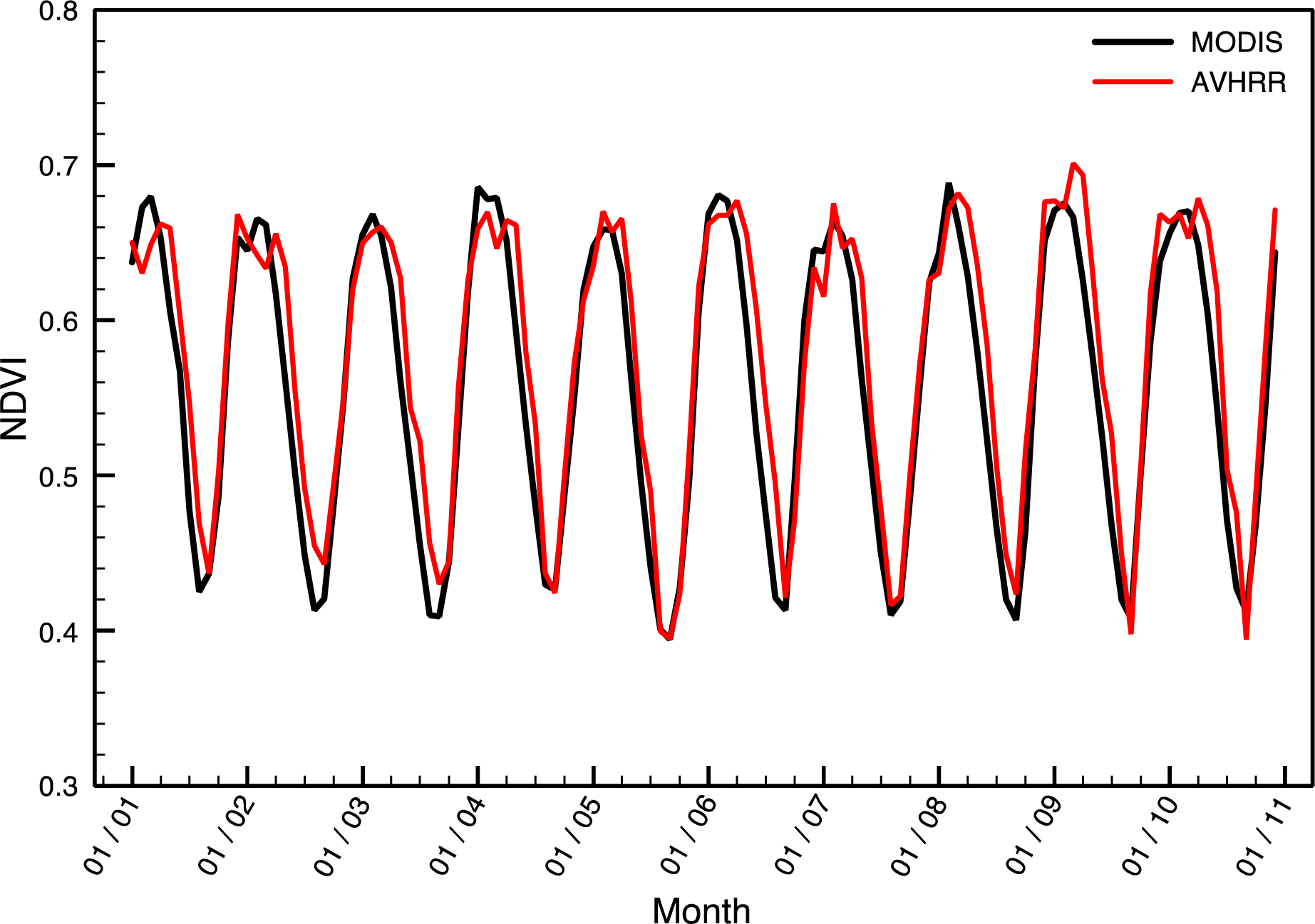
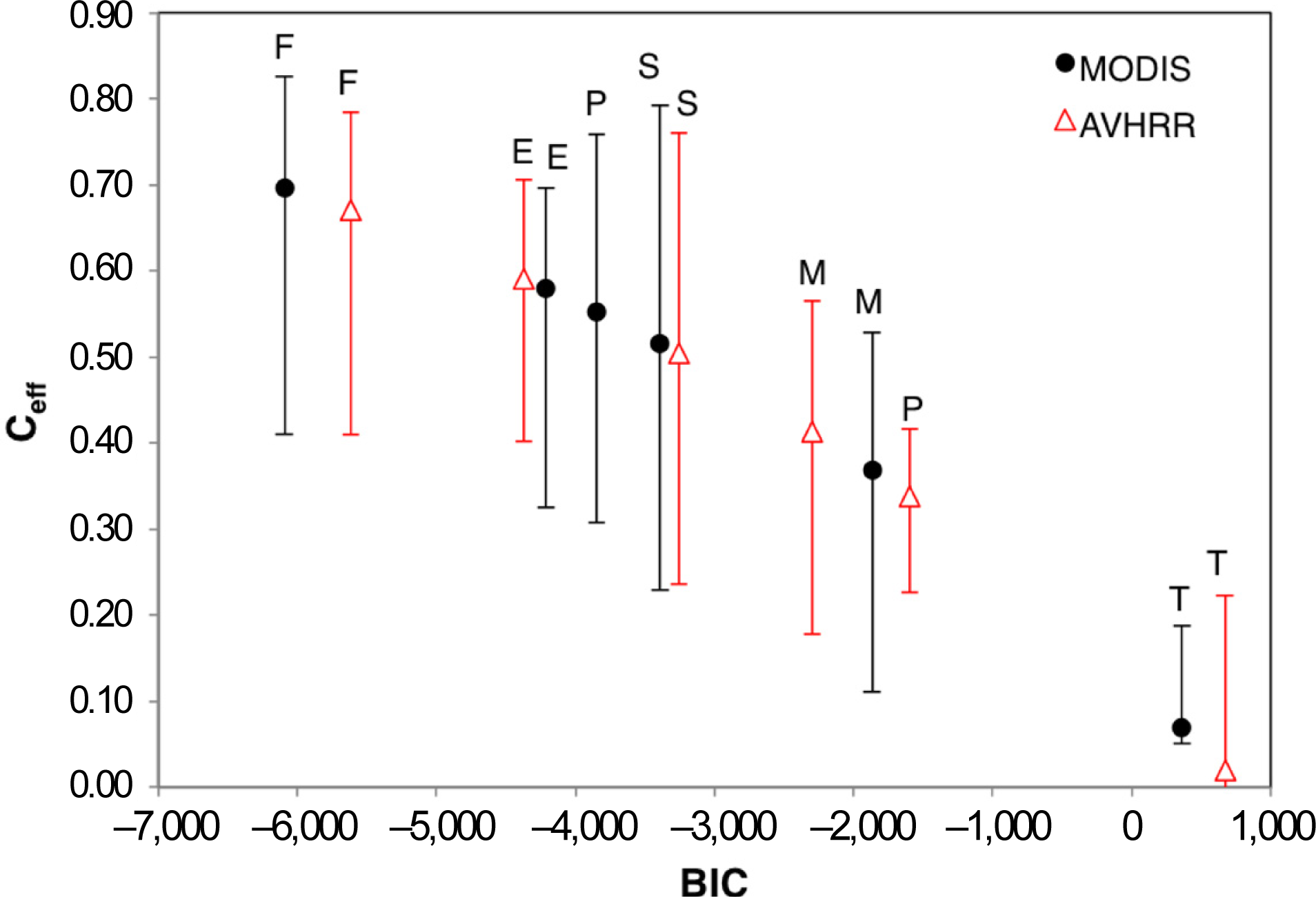
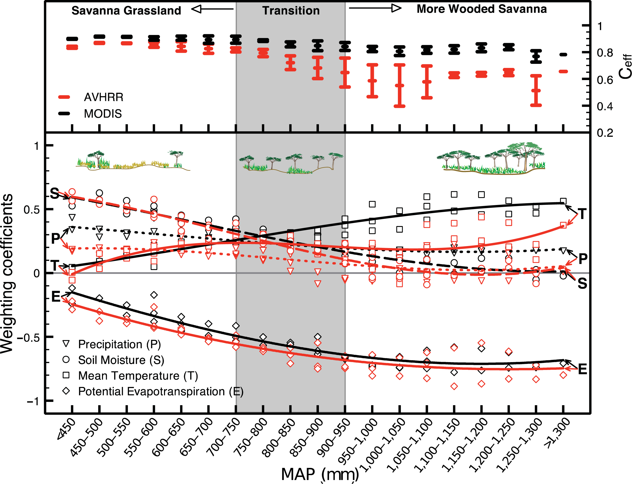
3.1. Part I: Comparison of MODIS and AVHRR Models (2001–2010)
3.2. PART II: Long-Term AVHRR Models (1982–2010)
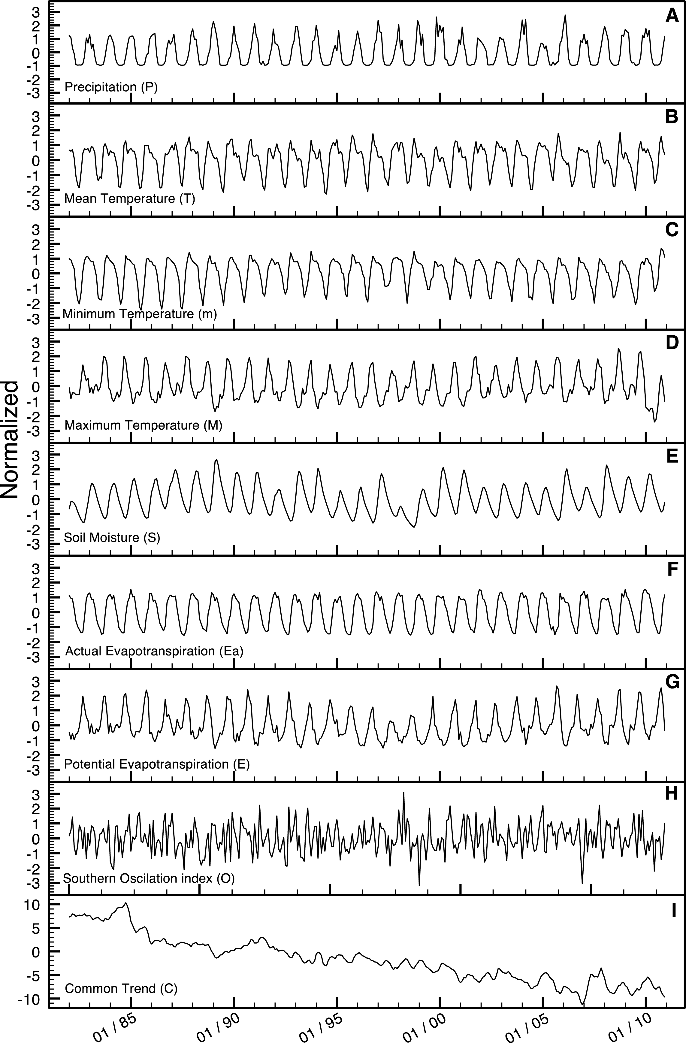
3.2.1. Experimental Time Series
3.2.2. Selection of Candidate Explanatory Variables
3.2.3. DFA Models (I, II and III)
4. Discussion
5. Conclusions
Acknowledgments
Conflicts of Interest
References
- Good, S.P.; Caylor, K.K. Climatological determinants of woody cover in Africa. Proc. Natl. Acad. Sci. USA 2011, 108, 4902–4907. [Google Scholar]
- Sankaran, M.; Hanan, N.P.; Scholes, R.J.; Ratnam, J.; Augustine, D.J.; Cade, B.S.; Gignoux, J.; Higgins, S.I.; Le Roux, X.; Ludwig, F.; et al. Determinants of woody cover in African savannas. Nature 2005, 438, 846–849. [Google Scholar]
- Sankaran, M.; Ratnam, J.; Hanan, N. Woody cover in African savannas: The role of resources, fire and herbivory. Glob. Ecol. Biogeogr 2008, 17, 236–245. [Google Scholar]
- Seghieri, J.; Vescovo, A.; Padel, K.; Soubie, R.; Arjounin, M.; Boulain, N.; de Rosnay, P.; Galle, S.; Gosset, M.; Mouctar, A.H.; et al. Relationships between climate, soil moisture and phenology of the woody cover in two sites located along the West African latitudinal gradient. J. Hydrol 2009, 375, 78–89. [Google Scholar]
- Gillson, L.; Hoffman, M.T. Rangeland ecology in a changing world. Science 2007, 315, 53–54. [Google Scholar]
- Ringrose, S.; Matheson, W.; Tempest, F.; Boyle, T. The development and causes of range degradation features in southeast Botswana using multitemporal landsat mss imagery. Photogramm. Eng. Remote Sens 1990, 56, 1253–1262. [Google Scholar]
- Barnes, R.F.W. Effects of elephant browsing on woodlands in a Tanzanian national park: Measurements, models and management. J. Appl. Ecol 1983, 20, 521–539. [Google Scholar]
- Baxter, P.W.J.; Getz, W.M. A model-framed evaluation of elephant effects on tree and fire dynamics in African savannas. Ecol. Appl 2005, 15, 1331–1341. [Google Scholar]
- Ntumi, C.P.; van Aarde, R.J.; Fairall, N.; de Boer, W.F. Use of space and habitat by elephants (Loxodonta Africana) in the Maputo Elephant Reserve, Mozambique. S. Afr. J. Wildl. Res 2005, 35, 139–146. [Google Scholar]
- Hamandawana, H.; Chanda, R.; Eckardt, F. Reappraisal of contemporary perspectives on climate change in southern Africa’s Okavango Delta sub-region. J. Arid Environ 2008, 72, 1709–1720. [Google Scholar]
- Bucini, G.; Hanan, N.P. A continental-scale analysis of tree cover in African savannas. Glob. Ecol. Biogeogr 2007, 16, 593–605. [Google Scholar]
- Murphy, B.P.; Bowman, D.M.J.S. What controls the distribution of tropical forest and savanna? Ecol. Lett 2012, 15, 748–758. [Google Scholar]
- Zhu, L.; Southworth, J. Disentangling the relationships between net primary production and precipitation in southern Africa savannas using satellite observations from 1982 to 2010. Remote Sens 2013, 5, 3803–3825. [Google Scholar]
- Vrieling, A.; de Leeuw, J.; Said, M.Y. Length of growing period over Africa: Variability and trends from 30 years of NDVI time series. Remote Sens 2013, 5, 982–1000. [Google Scholar]
- De Jong, R.; Verbesselt, J.; Zeileis, A.; Schaepman, M.E. Shifts in global vegetation activity trends. Remote Sens 2013, 5, 1117–1133. [Google Scholar]
- Zhu, Z.; Bi, J.; Pan, Y.; Ganguly, S.; Anav, A.; Xu, L.; Samanta, A.; Piao, S.; Nemani, R.R.; Myneni, R.B. Global datasets of vegetation Leaf Area Index (LAI)3g and Fraction of Photosynthetically Active Radiation (FPAR)3g derived from Global Inventory Modeling and Mapping Studies (GIMMS) Normalized Difference Vegetation Index (NDVI3g) for the period 1981 to 2011. Remote Sens 2013, 5, 927–948. [Google Scholar]
- Mao, J.; Shi, X.; Thornton, P.E.; Hoffman, F.M.; Zhu, Z.; Myneni, R.B. Global latitudinal-asymmetric vegetation growth trends and their driving mechanisms: 1982–2009. Remote Sens 2013, 5, 1484–1497. [Google Scholar]
- Tucker, C.J.; Slayback, D.A.; Pinzon, J.E.; Los, S.O.; Myneni, R.B.; Taylor, M.G. Higher northern latitude normalized difference vegetation index and growing season trends from 1982 to 1999. Int. J. Biometeorol 2001, 45, 184–190. [Google Scholar]
- Zhang, X.Y.; Friedl, M.A.; Schaaf, C.B.; Strahler, A.H.; Hodges, J.C.F.; Gao, F.; Reed, B.C.; Huete, A. Monitoring vegetation phenology using MODIS. Remote Sens. Environ 2003, 84, 471–475. [Google Scholar]
- Zhou, L.M.; Tucker, C.J.; Kaufmann, R.K.; Slayback, D.; Shabanov, N.V.; Myneni, R.B. Variations in northern vegetation activity inferred from satellite data of vegetation index during 1981 to 1999. J. Geophys. Res.: Atmos 2001, 106, 20069–20083. [Google Scholar]
- Baret, F.; Guyot, G. Potentials and limits of vegetation indexes for LAI and APAR assessment. Remote Sens. Environ 1991, 35, 161–173. [Google Scholar]
- Piao, S.; Fang, J.; Zhou, L.; Ciais, P.; Zhu, B. Variations in satellite-derived phenology in China’s temperate vegetation. Glob. Change Biol 2006, 12, 672–685. [Google Scholar]
- Badeck, F.W.; Bondeau, A.; Bottcher, K.; Doktor, D.; Lucht, W.; Schaber, J.; Sitch, S. Responses of spring phenology to climate change. New Phytol 2004, 162, 295–309. [Google Scholar]
- Schwartz, M.D.; Ahas, R.; Aasa, A. Onset of spring starting earlier across the northern hemisphere. Glob. Change Biol 2006, 12, 343–351. [Google Scholar]
- Zhang, X.Y.; Friedl, M.A.; Schaaf, C.B.; Strahler, A.H. Climate controls on vegetation phenological patterns in northern mid- and high-latitudes inferred from MODIS data. Glob. Change Biol 2004, 10, 1133–1145. [Google Scholar]
- Zhang, X.; Tarpley, D.; Sullivan, J.T. Diverse responses of vegetation phenology to a warming climate. Geophys. Res. Lett 2007, 34, L19405. [Google Scholar]
- Kramer, K.; Leinonen, I.; Loustau, D. The importance of phenology for the evaluation of impact of climate change on growth of boreal, temperate and mediterranean forests ecosystems: An overview. Int. J. Biometeorol 2000, 44, 67–75. [Google Scholar]
- Zhang, X.Y.; Friedl, M.A.; Schaaf, C.B.; Strahler, A.H.; Liu, Z. Monitoring the response of vegetation phenology to precipitation in Africa by coupling MODIS and TRMM instruments. J. Geophys. Res.: Atmos 2005, 110, D12103. [Google Scholar]
- Peñuelas, J.; Filella, I.; Zhang, X.; Llorens, L.; Ogaya, R.; Lloret, F.; Comas, P.; Estiarte, M.; Terradas, J. Complex spatiotemporal phenological shifts as a response to rainfall changes. New Phytol 2004, 161, 837–846. [Google Scholar]
- Ciais, P.; Piao, S.-L.; Cadule, P.; Friedlingstein, P.; Chedin, A. Variability and recent trends in the African terrestrial carbon balance. Biogeosciences 2009, 6, 1935–1948. [Google Scholar]
- Seaquist, J.W.; Hickler, T.; Eklundh, L.; Ardo, J.; Heumann, B.W. Disentangling the effects of climate and people on sahel vegetation dynamics. Biogeosciences 2009, 6, 469–477. [Google Scholar]
- Anyamba, A.; Tucker, C.J. Analysis of sahelian vegetation dynamics using NOAA-AVHRR NDVI data from 1981 to 2003. J. Arid Environ 2005, 63, 596–614. [Google Scholar]
- Eklundh, L.; Olsson, L. Vegetation index trends for the African Sahel 1982–1999. Geophys. Res. Lett 2003, 30, 1430–1433. [Google Scholar]
- Fensholt, R.; Rasmussen, K.; Nielsen, T.T.; Mbow, C. Evaluation of earth observation based long term vegetation trends—Intercomparing NDVI time series trend analysis consistency of Sahel from AVHRR GIMMS, Terra MODIS and SPOT VGT data. Remote Sens. Environ 2009, 113, 1886–1898. [Google Scholar]
- Helldén, U.; Tottrup, C. Regional desertification: A global synthesis. Glob. Planet. Chang 2008, 64, 169–176. [Google Scholar]
- Jeyaseelan, A.T.; Roy, P.S.; Young, S.S. Persistent changes in NDVI between 1982 and 2003 over India using AVHRR GIMMS (Global Inventory Modeling and Mapping Studies) data. Int. J. Remote Sens 2007, 28, 4927–4946. [Google Scholar]
- Lanfredi, M.; Simoniello, T.; Macchiato, M. Temporal persistence in vegetation cover changes observed from satellite: Development of an estimation procedure in the test site of the Mediterranean Italy. Remote Sens. Environ 2004, 93, 565–576. [Google Scholar]
- McCloy, K.R.; Los, S.; Lucht, W.; Hojsgaard, S. A comparative analysis of three long-term NDVI datasets derived from AVHRR satellite data. EARSeL eProc 2005, 4, 52–56. [Google Scholar]
- Neeti, N.; Eastman, J.R. A contextual Mann-Kendall approach for the assessment of trend significance in image time series. Trans. GIS 2011, 15, 599–611. [Google Scholar]
- Olsson, L.; Eklundh, L.; Ardo, J. A recent greening of the Sahel—Trends, patterns and potential causes. J. Arid Environ 2005, 63, 556–566. [Google Scholar]
- Carvalho, L.M.T.; Fonseca, L.M.G.; Murtagh, F.; Clevers, J.G.P.W. Digital change detection with the aid of multiresolution wavelet analysis. Int. J. Remote Sens 2001, 22, 3871–3876. [Google Scholar]
- Andres, L.; Salas, W.A.; Skole, D. Fourier-analysis of multi temporal AVHRR data applied to a land-cover classification. Int. J. Remote Sens 1994, 15, 1115–1121. [Google Scholar]
- Anyamba, A.; Eastman, J. Interannual variability of NDVI over Africa and its relation to El Nino southern oscillation. Int. J. Remote Sens 1996, 17, 2533–2548. [Google Scholar]
- Crist, E.P.; Cicone, R.C. A physically-based transformation of Thematic Mapper data—The TM Tasseled Cap. IEEE Trans. Geosci. Remote Sens 1984, 22, 256–263. [Google Scholar]
- Jakubauskas, M.; Legates, D.; Kastens, J. Harmonic analysis of time-series AVHRR NDVI data. Photogramm. Eng. Remote Sens 2001, 67, 461–470. [Google Scholar]
- Engle, R.; Watson, M. A one-factor multivariate time-series model of metropolitan wage rates. J. Am. Stat. Assoc 1981, 76, 774–781. [Google Scholar]
- Geweke, J.F. The Dynamic Factor Analysis of Economic Time Series Models. In Latent Variables in Socio-Economic Models; Aigner, D.J., Goldberger, A.S., Eds.; North-Holland: Amsterdam, The Netherlands, 1977; pp. 365–382. [Google Scholar]
- Harvey, A.C. Forecasting, Structural Time Series Models and the Kalman Filter; Cambridge University Press: New York, NY, USA, 1989; p. 572. [Google Scholar]
- Lütkepohl, H. Introduction to Multiple Time Series Analysis; Springer: Berlin, Germany, 1991. [Google Scholar]
- Zuur, A.F.; Pierce, G.J. Common trends in northeast atlantic squid time series. J. Sea Res 2004, 52, 57–72. [Google Scholar]
- Kaplan, D.; Muñoz-Carpena, R.; Ritter, A. Untangling complex shallow groundwater dynamics in the floodplain wetlands of a southeastern U.S. coastal river. Water Resour. Res 2010, 46, W08528. [Google Scholar]
- Kovács, J.; Márkus, L.; Halupka, G. Dynamic factor analysis for quantifying aquifer vulnerability. Acta Geol. Hung 2004, 47, 1–17. [Google Scholar]
- Muñoz-Carpena, R.; Ritter, A.; Li, Y.C. Dynamic factor analysis of groundwater quality trends in an agricultural area adjacent to Everglades National Park. J. Contam. Hydrol 2005, 80, 49–70. [Google Scholar]
- Ritter, A.; Muñoz-Carpena, R. Dynamic factor modeling of ground and surface water levels in an agricultural area adjacent to Everglades National Park. J. Hydrol 2006, 317, 340–354. [Google Scholar]
- Kaplan, D.; Muñoz-Carpena, R. Complementary effects of surface water and groundwater on soil moisture dynamics in a degraded coastal floodplain forest. J. Hydrol 2011, 398, 221–234. [Google Scholar]
- Kisekka, I.; Migliaccio, K.W.; Munoz-Carpena, R.; Schaffer, B.; Li, Y.C. Dynamic factor analysis of surface water management impacts on soil and bedrock water contents in Southern Florida Lowlands. J. Hydrol 2013, 488, 55–72. [Google Scholar]
- Ritter, A.; Regalado, C.M.; Muñoz-Carpena, R. Temporal common trends of topsoil water dynamics in a humid subtropical forest watershed. Vadose Zone J 2009, 8, 437–449. [Google Scholar]
- Kuo, Y.; Wang, S.; Jang, C.; Yeh, N.; Yu, H. Identifying the factors influencing PM2.5 in southern Taiwan using dynamic factor analysis. Atmos. Environ 2011, 45, 7276–7285. [Google Scholar]
- Linares, J.C.; Tiscar, P.A. Buffered climate change effects in a mediterranean pine species: Range limit implications from a tree-ring study. Oecologia 2011, 167, 847–859. [Google Scholar]
- Linares, J.C.; Camarero, J.J. Growth patterns and sensitivity to climate predict silver fir decline in the Spanish pyrenees. Eur. J. For. Res 2012, 131, 1001–1012. [Google Scholar]
- Campo-Bescós, M.A.; Muñoz-Carpena, R.; Kaplan, D.A.; Southworth, J.; Zhu, L.; Waylen, P.R. Beyond precipitation: Physiographic gradients dictate the relative importance of environmental drivers on savanna vegetation. PLoS One 2013, 8, e72348. [Google Scholar]
- Linard, C.; Gilbert, M.; Snow, R.W.; Noor, A.M.; Tatem, A.J. Population distribution, settlement patterns and accessibility across Africa in 2010. PLoS One 2012, 7, e31743. [Google Scholar]
- Wint, G.R.W.; Robinson, T.P. Gridded Livestock of the World 2007; Food and Agriculture Organization of the United Nations (FAO): Rome, Italy, 2007; p. 131. [Google Scholar]
- McCarthy, T.S.; Cooper, G.R.J.; Tyson, P.D.; Ellery, W.N. Seasonal flooding in the Okavango Delta, Botswana—Recent history and future prospects. S. Afr. J. Sci 2000, 96, 25–33. [Google Scholar]
- Eswaran, H.; Almaraz, R.; vandenBerg, E.; Reich, P. An assessment of the soil resources of Africa in relation to productivity. Geoderma 1997, 77, 1–18. [Google Scholar]
- Legates, D.R.; Willmott, C.J. Mean seasonal and spatial variability in gauge-corrected, global precipitation. Int. J. Climatol 1990, 10, 111–127. [Google Scholar]
- Global Air Temperature and Precipitation Archive. Available online: http://climate.geog.udel.edu/~climate/html_pages/README.ghcn_ts2.html (accessed on 25 September 2013).
- Earth System Research Laboratory: Physical Sciences Division: The National Centers for Environmental Prediction-Department of Energy Atmospheric Model Intercomparison Project (NCEP-DOE AMIP) II Reanalysis. Available online: http://www.esrl.noaa.gov/psd/data/gridded/data.ncep.reanalysis2.html (accessed on 25 September 2013).
- Bureau-Southern Oscilllation Index (SOI) Archives. Available online: http://www.bom.gov.au/climate/current/soihtm1.shtml (accessed on 25 Semptember 2013).
- Fan, Y.; van den Dool, H. Climate prediction center global monthly soil moisture dataset at 0.5 degrees resolution for 1948 to present. J. Geophys. Res.: Atmos 2004, 109, D10102. [Google Scholar]
- Zuur, A.F.; Tuck, I.D.; Bailey, N. Dynamic factor analysis to estimate common trends in fisheries time series. Can. J. Fish. Aquat. Sci 2003, 60, 542–552. [Google Scholar]
- Dempster, A.; Laird, N.; Rubin, D. Maximum likelihood from incomplete data via EM algorithm. J. R. Stat. Soc. Ser. B Methodol 1977, 39, 1–38. [Google Scholar]
- Shumway, R.H.; Stoffer, D.S. An approach to time series smoothing and forecasting using the EM algorithm. J. Time Ser. Anal 1982, 3, 253–264. [Google Scholar]
- Wu, L.S.Y.; Pai, J.S.; Hosking, J.R.M. An algorithm for estimating parameters of state-space models. Stat. Probab. Lett 1996, 28, 99–106. [Google Scholar]
- Zuur, A.F.; Ieno, E.N.; Smith, G.M. Analysing Ecological Data; Springer: New York, NY, USA, 2007; p. 672. [Google Scholar]
- Nash, J.E.; Sutcliffe, J.V. River flow forecasting through conceptual models Part I—A discussion of principles. J. Hydrol 1970, 10, 282–290. [Google Scholar]
- Ritter, A.; Muñoz-Carpena, R. Performance evaluation of hydrological models: Statistical significance for reducing subjectivity in goodness-of-fit assessments. J. Hydrol 2013, 480, 33–45. [Google Scholar]
- Schwarz, G. Estimating dimension of a model. Ann. Stat 1978, 6, 461–464. [Google Scholar]
- Zuur, A.F.; Fryer, R.J.; Jolliffe, I.T.; Dekker, R.; Beukema, J.J. Estimating common trends in multivariate time series using dynamic factor analysis. Environmetrics 2003, 14, 665–685. [Google Scholar]
- Montgomery, D.R.; Peck, E.A. Introduction to Linear Regression Analysis; Wiley: New York, NY, USA, 1992. [Google Scholar]
- Kuo, Y.; Chang, F. Dynamic factor analysis for estimating ground water arsenic trends. J. Environ. Qual 2010, 39, 176–184. [Google Scholar]
- Ward, D.; Wiegand, K.; Getzin, S. Walter’s two-layer hypothesis revisited: Back to the roots! Oecologia 2013, 172, 617–630. [Google Scholar]
- Linhoss, A.; Muñoz-Carpena, R.; Kiker, G.; Hughes, D. Hydrologic modeling, uncertainty, and sensitivity in the Okavango Basin: Insights for scenario assessment: Case Study. J. Hydrol. Eng. 2013, in press. [Google Scholar]
- Farrar, T.J.; Nicholson, S.E.; Lare, A.R. The influence of soil type on the relationships between NDVI, rainfall, and soil moisture in semiarid Botswana. II. NDVI response to soil moisture. Remote Sens. Environ 1994, 50, 121–133. [Google Scholar]
- Richard, Y.; Poccard, I. A statistical study of NDVI sensitivity to seasonal and interannual rainfall variations in Southern Africa. Int. J. Remote Sens 1998, 19, 2907–2920. [Google Scholar]
- Staver, A.C.; Archibald, S.; Levin, S. Tree cover in sub-Saharan Africa: Rainfall and fire constrain forest and savanna as alternative stable states. Ecology 2011, 92, 1063–1072. [Google Scholar]


| Dataset | Symbol | Source |
|---|---|---|
| Matsuura and Willmott’s Monthly Precipitation | P | [67] |
| Matsuura and Willmott’s Monthly Mean Temperature | T | [67] |
| NCEP-DOE Reanalysis II Monthly Minimum Temperature | m | [68] |
| NCEP-DOE Reanalysis II Monthly Maximum Temperature | M | [68] |
| CPC Monthly Soil Moisture | S | [68] |
| Matsuura and Willmott’s Monthly Actual Evapotranspiration | Ea | [67] |
| NCEP-DOE Reanalysis II Monthly Potential Evapotranspiration | E | [68] |
| NCEP-DOE Reanalysis II Monthly Vapor Pressure Deficit | V | [68] |
| Monthly Southern Oscillation Index | O | [69] |
| NDVI | ||
|---|---|---|
| MODIS | AVHRR | |
| F | 0.70 (0.51–0.81) | 0.67 (0.42–0.79) |
| F S | 0.82 (0.70–0.87) | 0.80 (0.55–0.88) |
| F S P | 0.89 (0.81–0.92) | 0.81 (0.59–0.90) |
| F S P T | 0.90 (0.86–0.92) | 0.82 (0.66–0.90) |
| F S P T E | 0.91 (0.88–0.93) | 0.83 (0.66–0.91) |
| Variable Symbol | VIF | |
|---|---|---|
| Step 1 | Step 2 | |
| P | 4.9 | 4.4 |
| T | 9.8 | 8.4 |
| m | 9.8 | 8.6 |
| M | 12.1 | 5.5 |
| S | 2.2 | 2.1 |
| Ea | 11.5 | 7.2 |
| E | 7.5 | 5.5 |
| V | 33.9 | - |
| O | 1.0 | 1.0 |
| Modela | No. of Trends (C) | Explanatory Variables | No. of Parameters | BICb | Ceffc | p-valued | ρ1,ne |
|---|---|---|---|---|---|---|---|
| I | 1 | - | 1,272 | −8,186 | 0.79 (0.34–0.95) | + | 0.89 (0.59–0.97) |
| 2 | - | 1,319 | −8,083 | 0.79 (0.34–0.95) | + | ||
| 3 | - | 1,365 | −7,909 | 0.80 (0.37–0.95) | + | ||
| II | 1 | Ea | 1,320 | −8,256 | 0.78 (0.36–0.90) | + | 0.57 (0.33–0.68) |
| 1 | Ea M | 1,368 | −8,531 | 0.74 (0.37–0.87) | + | 0.06 (−0.01–0.11) | |
| 1 | Ea T S | 1,416 | −8,538 | 0.77 (0.46–0.87) | + | 0.06 (−0.01–0.11) | |
| 1 | Ea T S P | 1,464 | −8,293 | 0.79 (0.52–0.87) | + | 0.06 (−0.02–0.11) | |
| 1 | Ea T S P M | 1,512 | −8,027 | 0.81 (0.53–0.89) | + | 0.06 (−0.02–0.11) | |
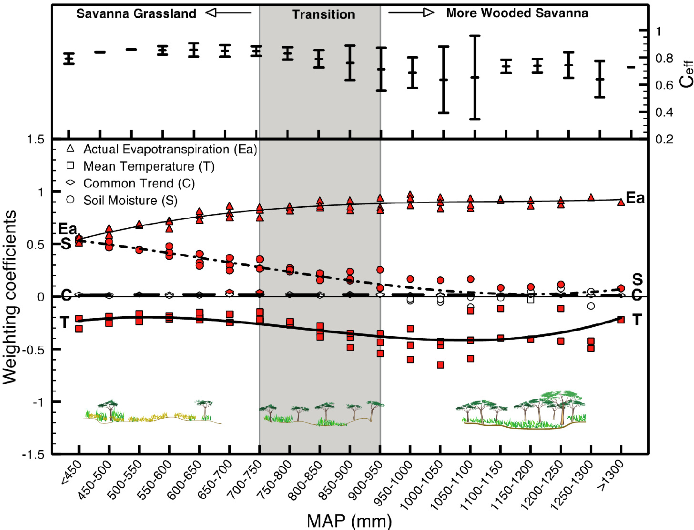
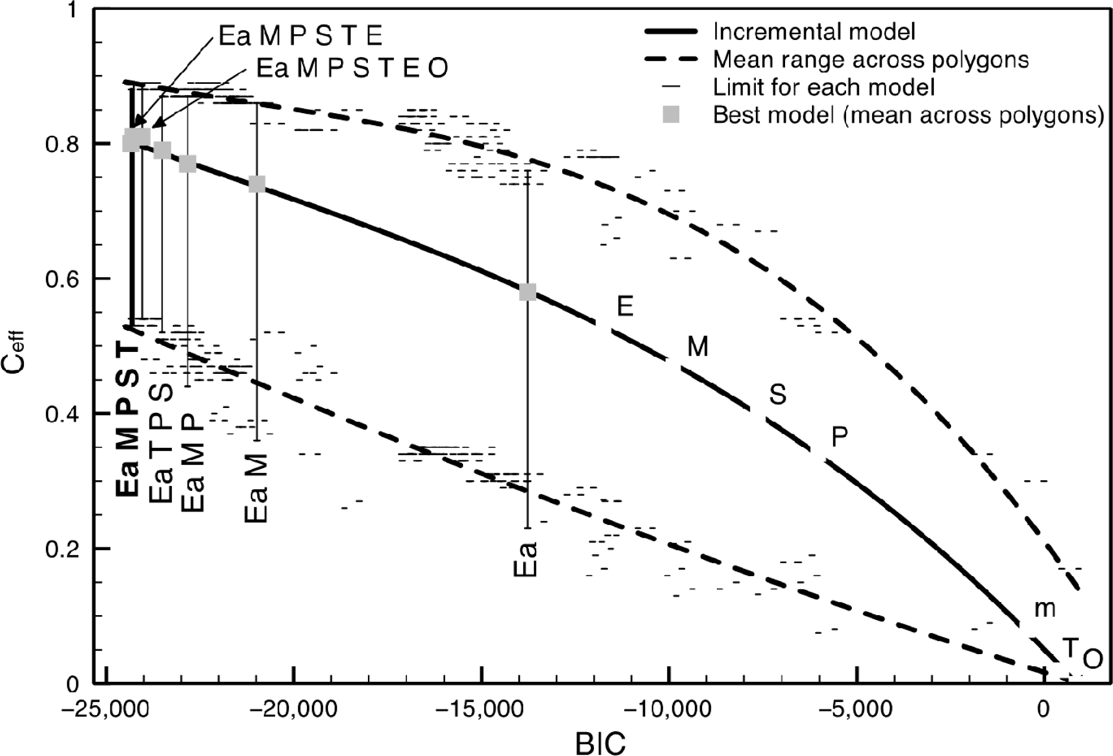
| III | 0 | Ea | 96 | −13,766 | 0.58 (0.23–0.76) | − | |
| 0 | Ea M | 144 | −20,980 | 0.74 (0.36–0.86) | + | ||
| 0 | Ea M P | 192 | −22,830 | 0.77 (0.44–0.87) | + | ||
| 0 | Ea T S P | 240 | −23,506 | 0.79 (0.52–0.87) | + | ||
| 0 | Ea T S P M | 288 | −24,333 | 0.80 (0.53–0.88) | + | ||
© 2013 by the authors; licensee MDPI, Basel, Switzerland This article is an open access article distributed under the terms and conditions of the Creative Commons Attribution license ( http://creativecommons.org/licenses/by/3.0/).
Share and Cite
Campo-Bescós, M.A.; Muñoz-Carpena, R.; Southworth, J.; Zhu, L.; Waylen, P.R.; Bunting, E. Combined Spatial and Temporal Effects of Environmental Controls on Long-Term Monthly NDVI in the Southern Africa Savanna. Remote Sens. 2013, 5, 6513-6538. https://doi.org/10.3390/rs5126513
Campo-Bescós MA, Muñoz-Carpena R, Southworth J, Zhu L, Waylen PR, Bunting E. Combined Spatial and Temporal Effects of Environmental Controls on Long-Term Monthly NDVI in the Southern Africa Savanna. Remote Sensing. 2013; 5(12):6513-6538. https://doi.org/10.3390/rs5126513
Chicago/Turabian StyleCampo-Bescós, Miguel A., Rafael Muñoz-Carpena, Jane Southworth, Likai Zhu, Peter R. Waylen, and Erin Bunting. 2013. "Combined Spatial and Temporal Effects of Environmental Controls on Long-Term Monthly NDVI in the Southern Africa Savanna" Remote Sensing 5, no. 12: 6513-6538. https://doi.org/10.3390/rs5126513