Use of Satellite Radar Bistatic Measurements for Crop Monitoring: A Simulation Study on Corn Fields

Abstract
: This paper presents a theoretical study of microwave remote sensing of vegetated surfaces. The purpose of this study is to find out if satellite bistatic radar systems can provide a performance, in terms of sensitivity to vegetation geophysical parameters, equal to or greater than the performance of monostatic systems. Up to now, no suitable bistatic data collected over land surfaces are available from satellite, so that the electromagnetic model developed at Tor Vergata University has been used to perform simulations of the scattering coefficient of corn, over a wide range of observation angles at L- and C-band. According to the electromagnetic model, the most promising configuration is the one which measures the VV or HH bistatic scattering coefficient on the plane that lies at the azimuth angle orthogonal with respect to the incidence plane. At this scattering angle, the soil contribution is minimized, and the effects of vegetation growth are highlighted.1. Introduction
A bistatic radar system is defined when antennas for reception and transmission are physically separated [1]. In principle, the transmitting and receiving antennas could be located on ground, on an aircraft or on-board a spacecraft; mixed solutions are also possible, e.g., the transmitter is spaceborne, while the receiver is airborne. The system could be either cooperating (transmitter and receiver designed for the specific bistatic application) or non-cooperating (transmitter designed independently of the receiver). If both receiver and transmitter, or illuminator, operate in the microwave band, the latter could be a radar, a communication or navigation satellite. For instance, non-cooperating systems can use already-existing satellite Synthetic Aperture Radars (SARs) as transmitters [2,3], as well as the signal transmitted by Global Positioning System (GPS) satellites [4,5]. Bistatic applications were investigated in the fields of target detection [6,7] and planetology [8]. As for Earth Observation, oceanographic studies exploiting the GPS signal were carried out, including altimetric applications (measure of the sea level and of the associated oceanographic features) and scatterometric applications (measure of the near surface wind field) [9,10], while interferometric applications were addressed in [11]. In consequence of the recent launch of the new generation of X-band radars (TerraSAR-X, COSMO-SkyMed), experiments involving X-band have been accomplished in order to evaluate the additional information contained in the bistatic reflectivity of targets (e.g., [12]). The TerraSAR-X mission has been extended into the TanDEM-X mission [13] with the purpose of generating global Digital Elevation Model from radar interferometry. This is the first bistatic system in orbit, and it successfully provided bistatic images of urban features [14]. However, its quasi-monostatic configuration does not appear suitable to observe vegetated surfaces whose directional scattering properties can be detected under large bistatic angles, as will be shown in this study.
The effect of soil moisture (SM) and roughness on the amplitude of the incoherent backscattered signal was largely investigated, and the effectiveness for their retrieval by radars working in the low-frequency range of the microwave band (1–5 GHz) was demonstrated (e.g., [15–19]). The sensitivity to vegetation parameters of monostatic radar measurements was assessed in [20,21], while the possibility to extract quantitative information on crop height from interferometric coherence and phase has been exploited in [22,23]. Up to now, few works are available on the use of a bistatic radar configuration for measuring land bio-geophysical parameters, such as vegetation and soil parameters. The first attempt to retrieve soil reflectivity and dielectric constant from Global Navigation Satellite System (GNSS) reflected data of the SMEX02 campaign was reported by [24], while in [25], the Interferometric Pattern Technique has been applied to retrieve the wheat crop height. The feasibility of retrieving SM using bistatic radar systems was assessed in [26], where a simulation study aiming at identifying the best bistatic configurations, in terms of incidence angle, observation direction, polarization and frequency band, for soil moisture content was performed. The technical issues related to the configurations selected in [26] have been discussed in [27].
As for vegetation, some airborne bistatic measurement campaigns at P-band have been carried out to find bistatic configurations allowing for the minimization of double bounce scattering from vertical trees in order to detect vehicles in forest concealment [28]. From a theoretical perspective, the MIMICS model was modified to allow the simulation of bistatic scattering from forests [29]. Like its monostatic version, Bi-MIMICS follows a first order approach, which, therefore, neglects multiple scattering contributions that, on the other hand, can be important at higher frequencies. The relevant features of scattering in the specular direction from soil covered by a vegetation canopy were theoretically analyzed in [30,31], on the basis of simulations carried out by using the fully polarimetric electromagnetic model developed at the Tor Vergata University of Rome and described in [32] (hereafter, the TOV model). The theoretical results indicated that such a bistatic system would maintain an appreciable sensitivity to the plant water content of crops and forest biomass over a considerably wider range than in the monostatic operation mode [30,31], because of the attenuation due to vegetation of the coherent specular reflection from the soil.
Extending the well-established TOV model to bistatic configurations different from the specular one, this paper investigates the bistatic radar potential in view of vegetation parameter estimation. The bistatic scattering simulations, provided herewith, focus on the identification of the configuration, which provides the most accurate crop height retrieval; in particular, corn plants are considered for this purpose. The sensitivity yielded by the selected bistatic configurations is compared with that of standard monostatic radar. Moreover, the potential of combining both measurements, considering that backscatter is expected to be measured by conventional SAR missions (multistatic case) is assessed. We have used the Cramér–Rao Lower Bound to quantify and compare the retrieval performances of the different configurations.
In Section 2, a summary of the electromagnetic model used to perform the bistatic simulations will be given, together with a description of the parameters used for the sensitivity analysis of the bistatic configurations carried out in the following Section 3. The directional properties of vegetation are deeply investigated and, in particular, it will be shown that co-polar bistatic measurements, acquired on a plane orthogonal with respect to the incidence one, show an interesting sensitivity to biomass. Finally, a bistatic configuration will be selected on the basis of the sensitivity analysis, and its performance will be compared against the one of a monostatic system.
2. The Methodology and the Selected Electromagnetic Model
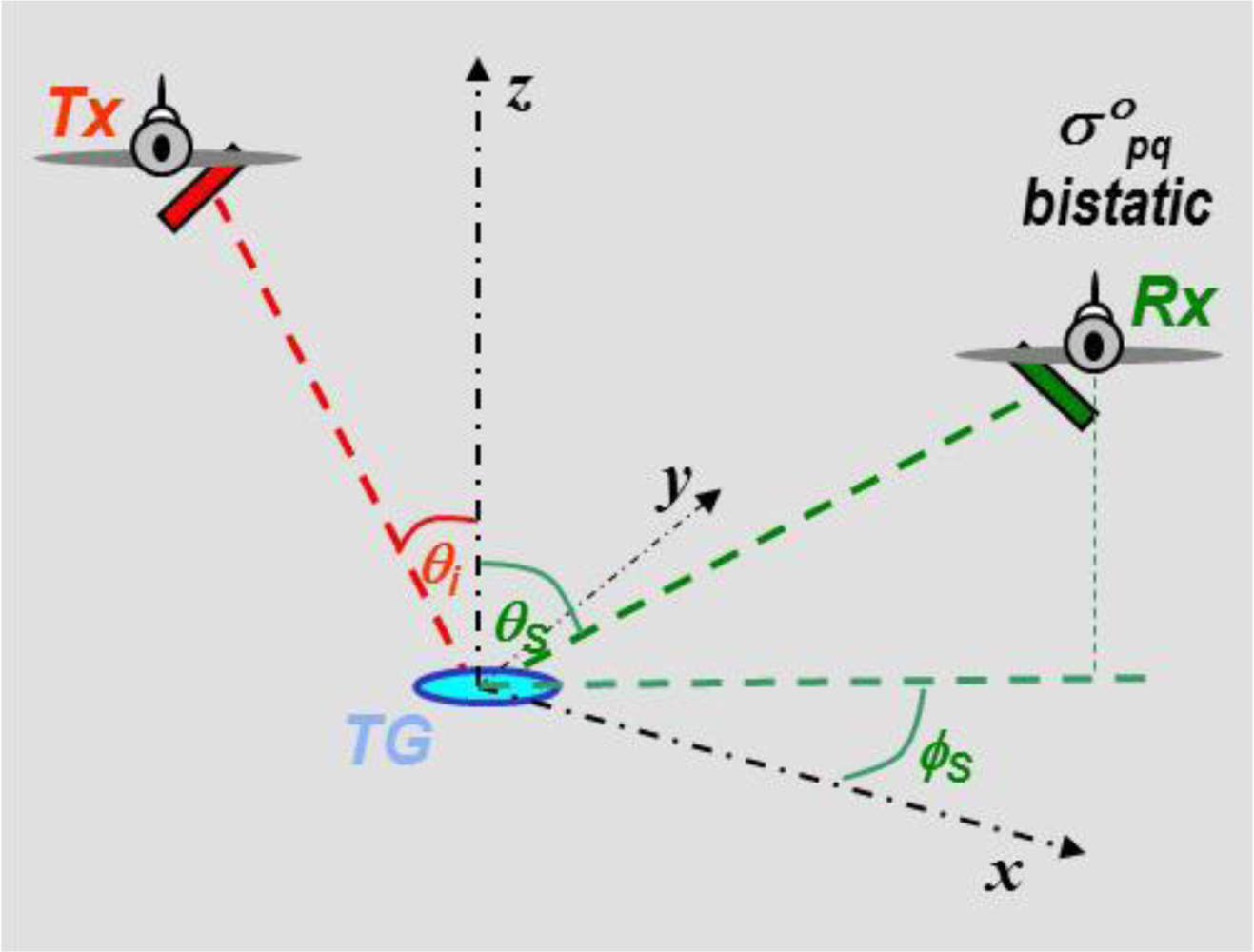
Bistatic configurations are defined in terms of frequency, polarization and transmitter-target-receiver relative geometry. This geometry is shown in Figure 1, in which the plane of incidence is assumed as a reference coordinate plane and the configuration is identified through the incidence angle (θi, red in Figure 1) with respect to the vertical, the zenith (θs) and azimuth (φs) scattering angles (green in Figure 1). The measurement performed by a bistatic radar consists in the bistatic scattering coefficient, i.e., the bistatic radar cross section per unit area:
In order to identify the set of bistatic system parameters (especially geometric parameters, but also polarization and frequency), which optimize the sensitivity to the crop height, the adopted methodology is based on a set of simulations of σ0 carried out by running the TOV model in correspondence of a range of system and target parameters. For the purpose of identifying the best configurations in terms of polarizations, incidence and scattering angles, the retrieval accuracy is quantified by using the Cramér–Rao Lower Bound (CRLB), already used in [26], which is based on the Bayesian theory of parameter estimation. Note that, even though forecasting the retrieval accuracy using simulations is a tricky problem, in this work, we are only interested on a relative comparison between the estimated retrieval performances in order to identify the optimal bistatic configurations. Although we cannot predict the actual accuracy without experimental data, this relative comparison is suitable for our purposes.
The selected electromagnetic model is described in the next section, with additional details reported in the Appendix. Then, some results of the simulations performed by running the model are presented.
The TOV model is fully polarimetric, since it can simulate the backscattering coefficient corresponding to any polarization of the incident and scattered power. However, in this work, simulations related to linear polarization only are discussed.
This section ends by describing the parameters chosen to identify the best configurations for crop status monitoring.
2.1. The Selected Electromagnetic Model
The TOV model, which has been selected to predict the bistatic scattering coefficient of crops, is based on the radiative transfer theory. It adopts a discrete approach [32] in which vegetation elements are described as discrete dielectric scatterers and suitable electromagnetic theories [33] are used to compute their absorption and scattering cross sections; in their turn, the latter are calculated using suitable permittivity models [34]. The soil is described as a homogeneous half-space with rough interface, producing surface scattering, which may be subdivided into two components: a coherent and an incoherent one. The coherent component is computed following the theory developed in [35], which takes the sphericity of the wavefront into account. The derived coherent scattering coefficient of the soil depends not only on the surface parameters, but also on the receiving and transmitting antenna parameters. In this study, the beamwidth of the receiving and transmitting antennas has been supposed to be equal to 3°. Furthermore, in order to account for coherent phenomena outside the plane of incidence, the formulation in [35] has been extended to any directions.
The incoherent bistatic scattering coefficient of soil is computed through the Integral Equation Model (IEM) [36]. Although several advances have been achieved in representing the statistics and the electromagnetic properties of soil surfaces, soil backscattering coefficient measured at HV polarization is generally underestimated by surface models, IEM included. On the other hand, experimental data point out that the backscattering coefficients at HV and VV polarizations are highly correlated. For this reason, we have linked the modeled σ0HV of bare soil to the modeled σ0VV of bare soil itself. This correction basically consists in multiplying the σ0VV IEM output by the average ratio between HV and VV backscattering measurements over bare soil available through the ERA-ORA library ( http://eraora.disp.uniroma2.it). The result is multiplied by the canopy transmission matrices at horizontal and vertical polarizations [20]. This semi-empirical correction has been applied to backscattering only, due to the lack of experimental bistatic data, which would be required to calculate the correction factor at every direction.
In order to combine vegetation and soil contributions, the TOV model adopts the Matrix Doubling algorithm [32] that accounts for the multiple scattering effects that take place between vegetation elements and the terrain. The main steps of the extension of the TOV model to the bistatic case are reported in the Appendix. As for the coherent component, attenuation by the vegetation layer has been superimposed to the soil contribution mentioned previously.
We recall here that model simulations showed a good fitting with polarimetric backscattering signatures measured over sunflower fields at L-band and two angles [32], bearing an error of about 1.5 dB at all polarizations over developed crops. The same model was able to explain the polarimetric features observed over several kinds of agricultural and forest areas at P-, L- and C-band [37]. Recently, the model simulated the backscattering signatures of wheat and corn at C-band [20,33], and in these cases, the accuracy was also good (less than 1.5 dB) for developed crops. The validation of the bistatic model for vegetation cannot be performed, because of the lack of suitable experimental data. Nevertheless, the ability of the model to predict the surface reflectivity, that is, the integral of the bistatic scattering coefficient over all the scattering directions, can be assessed. In fact, one minus the reflectivity provides the surface emissivity, which has been measured and compared with vegetation conditions in many experiments. Validations of the surface emissivity computed by the model have been carried out in [38,39], with a resulting accuracy equal to 0.02 at the L-band and to 0.04 at the C-band.
2.2. The Corn Crop Scenario
The reliability and accuracy of a theoretical model depends on its capacity to reproduce real measurements and, as just mentioned, the Tor Vergata model has been tested and validated against data collected under different conditions. Furthermore, a reliable model can also be used to predict measurements in order to evaluate the potential of a novel system. The model must then ensure the correct electromagnetic representation of the processes under study, but also a correct representation of the environmental scenario to be observed. To this end, the TOV model is made up of an electromagnetic module and of a growth module.
Indeed, the TOV model takes plant height as an input parameter, and it includes equations that, for a given height, calculate all other vegetation parameters, which are used to model corn bistatic scattering, i.e., leaf area index, leaf dimensions and moisture content, twigs dimensions, density and moisture content, stem dimensions, density and moisture content. As a consequence, all these parameters vary simultaneously in a realistic way, since the regression equations implemented within the TOV model have been established on the basis of ground truth measurements performed in the course of past various remote sensing campaigns. Most of them were derived by ground measurements collected during experimental campaigns carried out in the Central Plain site in Switzerland and can be found in table format in [33]. Therefore, the results presented in this study consist of theoretical simulations of bistatic measurements over a realistic corn crop scenario.
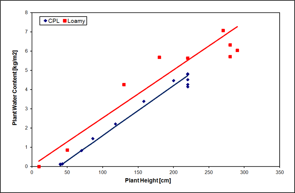
The sensitivity study carried out here is focused on the capability to retrieve plant height, from which it is possible to get information about the vegetation biomass. Height is related to plant water content in a way that depends on geographical characteristics and on working procedures of the agricultural site. As an example, in Figure 2, the measured plant height and water content of two corn sites, in Switzerland and Belgium [33], are shown together with regression lines. The reference corn crop scenario of this paper is the Central Plain one, and the plant heights considered for the sensitivity study are 50 and 100 cm. This means that the other plant parameters, such as Leaf Area Index, dimensions, moisture content, etc., vary in such a way to give a Plant Water Content equal to about 0.15 and 2 kg/m2, respectively.
In order to take into account different plant developments with respect to that of the Central Plain (like in the Belgian site reported in Figure 2), the plant coverage fraction has been introduced as an additional input parameter, besides plant height. In particular, a plant cover fraction increasing with plant height faster than at the Central Plain has been also considered in some of the examples presented in the following sections. This situation can correspond to more intensive agricultural practices.
2.3. Simulations Results
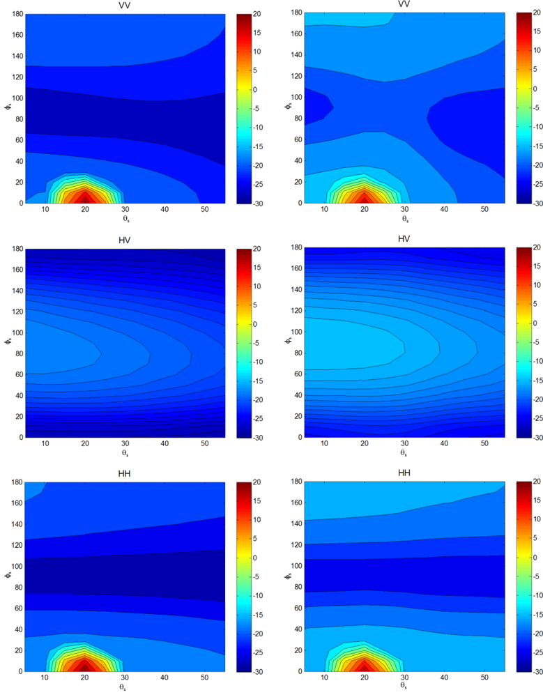
The bistatic TOV model has been run in order to simulate the bistatic scattering of corn fields, and the results are outputted as a matrix whose rows represent the scattering azimuth angles and whose columns represent the scattering look angles. In order to represent the bi-dimensional scattering properties of this vegetation medium, a color map has been used, as that reported in Figure 3, where colors represent the bistatic scattering coefficient values, with shades towards the red representing highest scattering and shades toward the blue the lowest scattering. In these maps, the horizontal axis represents the scattering look angle θs in the range [5°, 55°]; the vertical axis represents the azimuth scattering angle φs in the range [0°, 180°]. Due to the azimuthal symmetry of the vegetated medium, symmetric bistatic scattering coefficient values are expected for 180 ≤ φs ≤ 360. In the color map representation, the backscattering coefficient can be found on the upper side of the maps (φs = 180°; θs = θi), whereas the specular direction lies on the bottom (φs = 0°; θs = θi).
In Figure 3, the L-band is considered, and a soil characterized by SM = 10% and by a standard deviation of surface height (σz, representing roughness) of 0.5 cm has been assumed. Two values of corn height have been considered, i.e., 50 cm (low/moderate stage of growth) and 150 cm (well-developed plant). Looking at Figure 3, it can be noted that, in the co-polarized cases, the highest scattering is encountered toward the specular direction (φs = 0°; θs = θi = 20°). In this direction, coherent scattering from the soil is very strong, and it is only partially attenuated by the above lying vegetation. The lowest co-polar scattering is met at horizontal polarization on the plane orthogonal to the incidence one (φs = 90°), while on this same plane, the highest cross-polarized scattering occurs. This behavior is due to a reversal of the polarization vectors on the orthogonal plane, with respect to the polarization vectors defined in the plane of incidence. Indeed, the horizontal polarization vector defined in the plane of incidence, is seen as a vertical polarization vector on the plane with φs = 90°. Conversely, the vertical polarization vector defined in the plane of incidence is partially seen as a horizontal polarization vector on the plane with φs = 90°.
The increase of plant height (compare right and left column of Figure 3) determines an increase of vegetation volume scattering and an attenuation of soil scattering. The magnitude of these two contributions depends on the field plant cover fraction, but the bistatic scattering directional pattern does not. The results presented in Figure 3 refer to cover fractions of 20% at 50 cm height and 60% at h = 150 cm, which were recorded in the field measurements performed in the Central Plain site [20]. It has been found that an increase of plant coverage means a higher attenuation of the coherent contribution, besides a volume scattering contribution more significant with respect to soil contribution (especially for the highest plant). Consequently, the bistatic scattering coefficients are larger, except around the specular direction, where a decrease is observed.
The effects of increasing soil roughness or moisture content are to increase bistatic scattering in most of the scattering directions, due to a higher soil contribution, which is visible due the incomplete coverage of crop (60%) and to higher interactions between soil and vegetation. However, it has been found (not shown in this paper) that, around the specular direction, an increase of roughness causes a decrease of coherent scattering, while an increase of moisture content causes an increase in all directions.
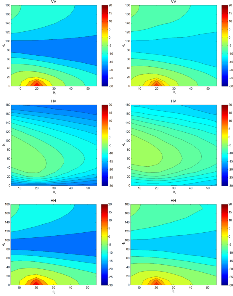
Changing incidence angle does not change the considerations previously drawn for θi = 20°, bearing in mind that the high incidence angles give rise to a lower scattering, for any soil roughness and moisture content. At C-band, where volume scattering is more significant and gives rise to a general increase of bistatic σ0 values (except, of course, for the specular direction, where an increase of attenuation produces a decrease of scattering), the angular trends are in general analogous to those at L-band (as it can be deduced by comparing Figure 4 and Figure 3). From Figure 4, it can be appreciated as at C-band the contrast between specular direction and the other directions is reduced (the color scale used in all these σ0 maps is unique, so their color can be directly compared).
2.4. Parameters for the Evaluations of the Bistatic Configurations
The retrieval accuracy of a given relevant target parameter (here, the crop height) obviously depends on the sensitivity of the measurement (the bistatic scattering coefficient, in this case) to the parameter itself. In order to evaluate the sensitivity to plant height, the soil parameters have been kept constant, and the following incremental ratio has been calculated from the model output:
Besides the sensitivity, the Cramér–Rao Lower Bound (CRLB) index has been used to better evaluate the potentiality of bistatic measurements and multistatic ones (that foresee the exploitation of the monostatic data, too, see Section 3) for retrieving the height of a corn plant. It is derived from the Bayes theory of parameter estimation and already used in [26]. Let us assume that we perform several measurements, σ01,σ02,…,σ0n (different polarizations and/or observation directions and/or frequencies), i.e., that we measure a n-component vector σ0 to estimate a given target parameter xi. The measurements do not depend only on xi, but also on other parameters, xj, that act as nuisance parameters. CRLB gives the best achievable accuracy of any unbiased estimator. By assuming a Gaussian measurement error with zero mean and a common variance, σn2, the minimum variance of the estimate, x̂i, is defined by the following inequality [26]:
CRLB is a positive quantity; the numerator contains the sensitivity to the nuisance parameter, x2, so that the greater the numerator, the larger the variance of the estimator. As for the denominator, it is equal to the determinant of [J(x)]T[J(x)]. Although it could be expected an increase of the denominator (i.e., an improvement of the retrieval performance) if the sensitivity to the target parameter rises, this condition is not sufficient to achieve a reliable estimation of the x1 parameter. In fact, if the term (J11J12 + J21J22)2 compensates for the term , CRLB tends to rise. Such compensation occurs if the different measurements have similar sensitivity to the bio-geophysical parameter to be estimated (the crop height in this case), so that the determinant of [J(x)]T[J(x)] becomes close to zero. In other words, to ensure a reliable estimation of x1, the sensitivity to x1 must be high, and the various measurements must provide non-redundant information. The CRLB diverges to infinity when only one measurement is available or the Jacobian matrix is singular, since in both cases it is not possible to solve for the two unknowns x1 and x2.
Note that introducing in Equation (4) a constant average value of the sensitivity, as it will be done in the sequel, corresponds to assuming that the forward problem is linear. If we compute the sensitivity around different values of the parameter (for instance computing sensitivity to plant height for small, medium and tall plants), we could obtain slightly different results. However, here, we are interested to find the bistatic configuration, which provides on average the best retrieval performance, so that the consideration of an average sensitivity within a large range of the target parameters is justified.
3. Analysis of the Bistatic Configurations for Crop Height Monitoring
3.1. Analysis of the Sensitivity of Single Polarization Data
As previously stated, the sensitivity analysis for the vegetated target has been carried out by considering corn, which is one of the world most common agricultural crops. In order to explore a wide range of bistatic configurations (polarizations and geometry) with a reasonable number of model runs, the system parameters reported in Table 1 have been chosen.
Furthermore, two frequencies, i.e., 1.2 GHz (L-band) and 5.3 GHz (C-band), have been considered. As discussed in Section 2, scattering from vegetated areas is also influenced by soil roughness and moisture. In order to simulate the variability of soil conditions, the parameters reported in Table 2 have been chosen as representative of smooth and rough soils and dry and moist soil beneath vegetation. The above roughness parameters meet the IEM applicability criteria (which can be found in graphical form in [40]) at the frequencies of interest.
The following sensitivity analysis will be performed on single configuration data, that is, assuming that the measurement is acquired along a single observation direction.
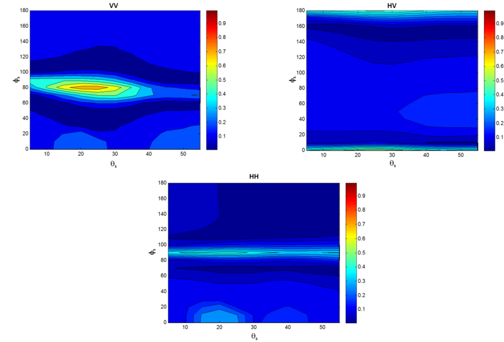
The sensitivity to plant height is defined by Equation (2). From the sensitivity point of view, a negative and a positive value of the incremental ratio, defined by Equation (2), are equivalent. For this reason, the absolute value will be considered hereafter. However, it must be underlined that, around the specular direction (where the coherent soil component is generally predominant), a negative Δσ0/Δh is obtained, differently from all other directions. The sensitivity maps are given in units of dB/(10 cm); blue represents a low sensitivity, while red corresponds to a high sensitivity.
The above plots (Figure 5) refer to simulations carried out at L-band for two corn plant heights (h = 50 and 150 cm), as representative of young and well-developed corn plants, and the soil parameters are SM = 25% and σz = 1.5 cm. Figure 5 shows that the maximum sensitivities of bistatic σ0 are shown at different directions, depending on the polarization: at horizontal polarization, it occurs on the scattering plane orthogonal to the incidence one, that is, for directions with φs = 90°; at vertical polarization for some directions with φs ∼ 80°; at cross-polarization, on directions contained in the plane of incidence, both in the backward (φs = 180°) and forward (φs = 0°) semi-planes. All this happens because, on these planes, the soil contribution is very low and the vegetation growth gives rise to increasing volume scattering (at HH or HV polarizations) or interaction with soil (at vertical polarization). Among the three polarizations, the vertical one shows the maximum sensitivity that, depending on soil conditions and observation angle, can reach more than 0.9 dB/(10 cm), which is considerably higher than that exhibited for the monostatic case. The latter, corresponding to θs = θi = 20° and φs = 180°, exhibits a sensitivity not larger than 0.3 dB/10 cm. At other polarizations, the maximum obtained value is 0.5. In the case study of Figure 5, the specular configuration does not provide good sensitivities, because of the low cover fraction characterizing the corn field: indeed, in the specular direction the coherent soil contribution is the dominant one, but attenuation introduced by the crop is not enough to produce a significant change of σ0 in the specular direction.
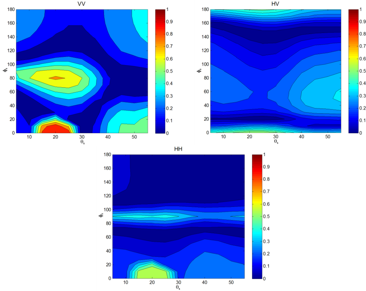
As mentioned in Section 2, a plant cover fraction of approximately 60% has been assumed for the tallest plant, whereas for h = 50 cm, the 20% of coverage has been assumed. We have also increased these fractions (to 100% and 40%, respectively), obtaining higher volume scattering and attenuation. The latter produces an increase of sensitivity in the specular direction, while volume scattering produces a general increase of sensitivity that, as it can be observed in Figure 6, is more or less remarkable, depending on the bistatic scattering angles. The general angular trend keeps, however, the same behavior. Even with this kind of phenology, the best sensitivities are presented by vertical polarization at φs∼80° and θs∼20°, besides the specular direction.
Indeed, the sensitivity in the specular configuration is connected to the attenuation by the plant canopy, which makes it very suitable to vegetation biomass monitoring. The scattering phenomena, which take place in this direction, were theoretically analyzed in [30,31], so that considerations on this specific configuration are excluded from the present study.
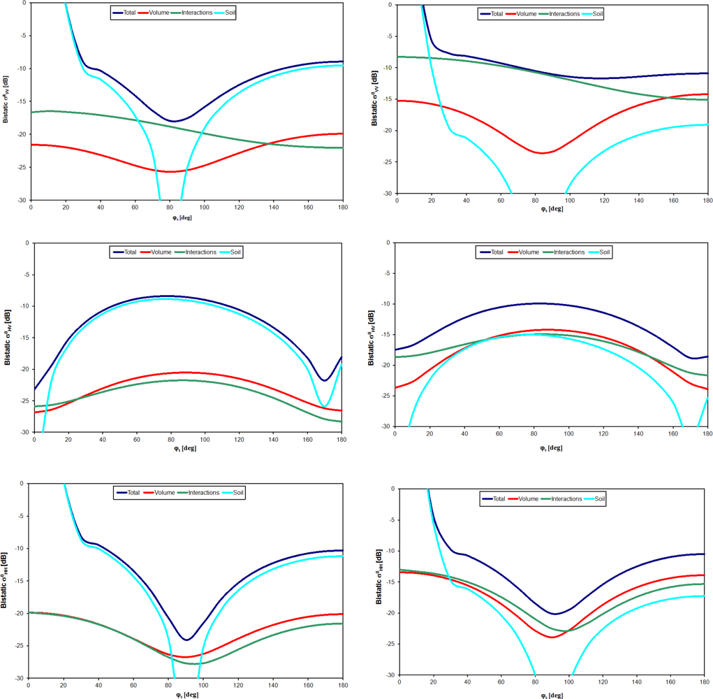
In order to understand this behavior, we singled out the contributions originating from the various scattering sources along the directions, which presented the maximum variability of sensitivity, i.e., along the so-called “forward scattering cone”. In the following figures (Figure 7, corresponding to input parameters, as in Figure 6), scattering contribution from the vegetation volume, interactions between vegetation and soil—including double bounce—and the soil contribution are shown as a function of the azimuth scattering angle φs, once the incidence and scattering look angles have been fixed equal to 20°. A corn canopy in the early development (i.e., with h = 50 cm and 40% vegetation cover) and a fully developed one (h = 150 cm, cover of 100%) are considered on the left and right columns, respectively. In backscattering (φs = 180°), soil contribution is dominant at L-band for short plants, as expected. For fully developed plants, volume scattering and interaction effects are important. In the specular direction, soil coherent scattering gives rise to a high co-polar bistatic scattering coefficient. However, it can be observed from the plots that the relative weights of the various contributions are azimuth-dependent. Volume scattering and, mainly, the soil contribution show the minimum value of bistatic σ0HH on the direction at azimuth scattering angle φs = 90°, that is, orthogonal with respect to the plane of incidence, and at the same scattering angle, they are maximum at cross-polarization. At vertical polarization, the minimum is slightly shifted toward φs ∼ 80°.
We can conclude that the maximum sensitivity to plant height is displayed when the soil contribution is very low and the plant growth can appear with the maximum contrast.
The effects of changing incidence direction (i.e., θi = 35° and 50°) have been studied, and it has been observed that the considerations drawn previously still apply. In particular, the highest sensitivities at horizontal polarization appear on the orthogonal plane (φs = 90°) and on the backward plane (φs∼180°) at cross-polarization. As far as the vertical polarization is concerned, a shift of the bistatic direction showing the best sensitivity is observed. In particular, for θi = 35°, the best sensitivity is shown at θs = 35°, φs = 70°. This effect is due to the fact that the direction at which the soil contribution shows its minimum is dependent on the incidence direction, according to the IEM simulations of soil bistatic scattering [36] (p. 266) We also note that the sensitivity decreases with increasing incidence angle. The best sensitivity to corn plant height is therefore shown at vertical polarization in the bistatic configuration with θi = 20° and φs = 80°, θs = 20°.
The sensitivity to plant height has been evaluated at C-band too. Although it is reduced with respect to L-band, it is still significant at vertical polarization at the same angles of the lower frequency. At C-band, the two co-polar linear polarizations show similar values (around 0.5 dB/(10 cm)), with horizontal polarization showing the best sensitivity on the “orthogonal” scattering plane.
3.2. CRLB for Multipolarization Data
In this section, it will be assumed that measurements at two polarizations, with the same bistatic observation direction, are available. It is understood that this analysis includes the special case of the observation of backscattered waves. Three different possible combinations of polarization are considered: bistatic measurements at VV and VH polarizations, bistatic measurements at HH and HV polarizations and bistatic measurements at VV and HH polarizations. To evaluate the performance of these multipolarized bistatic systems, the CRLB defined in Section 2 was computed. As previously discussed, this parameter is more powerful than just looking at the sensitivity, if one wants to analyze a multidimensional data set. The parameter to be monitored (x1) is the corn plant height, h, the nuisance parameter (x2) has been supposed to be the soil moisture content, while the soil roughness has been assumed to be constant (i.e., σz = 1.5 cm). The standard deviation error of the measurements σn has been supposed to be 1 dB.
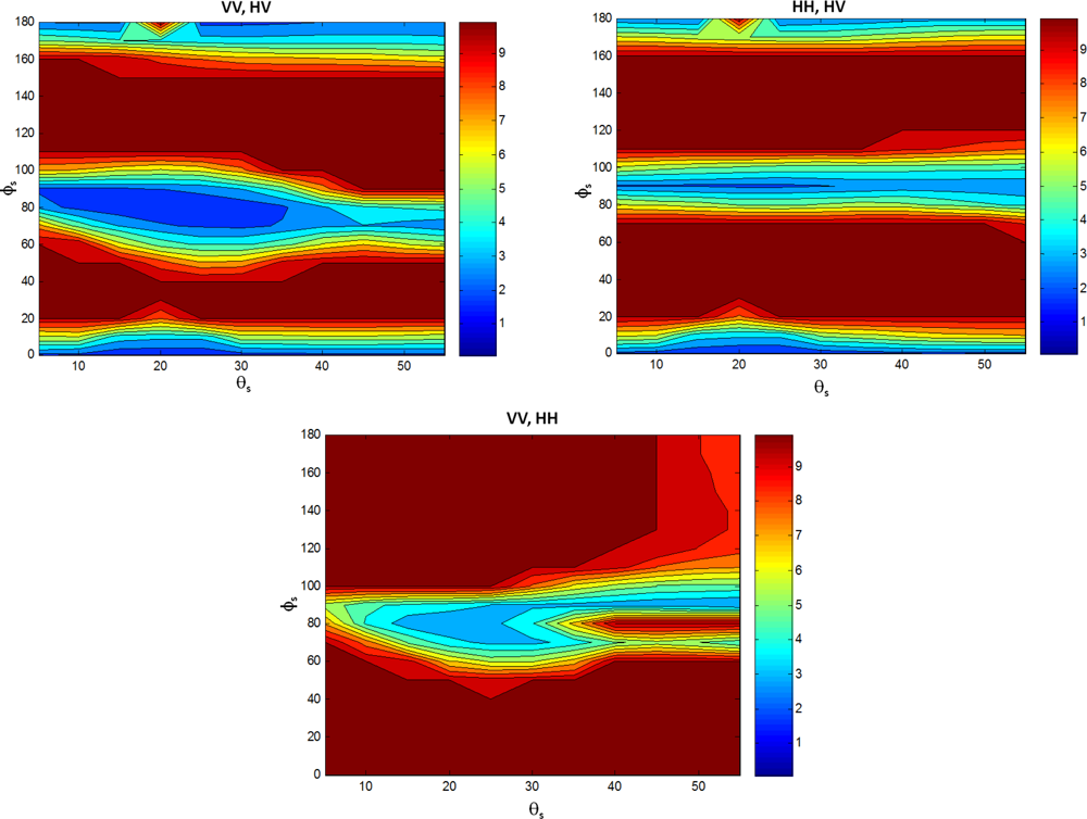
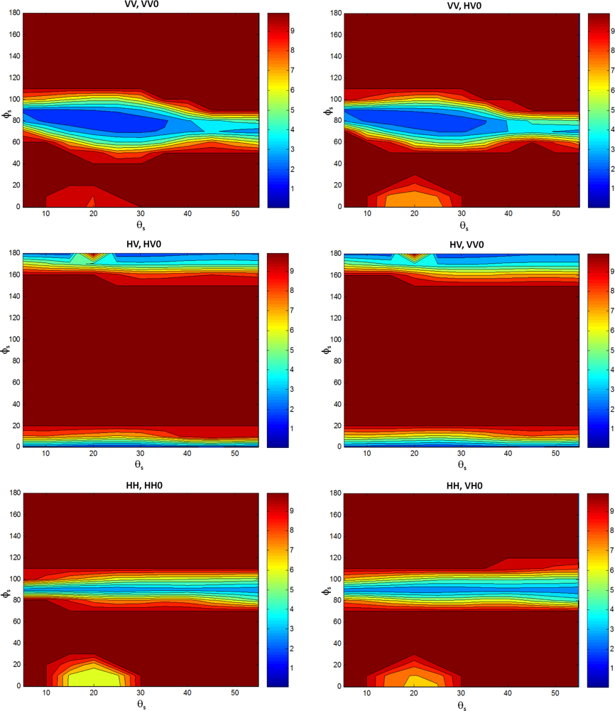
In the maps presented in Figure 8, the square root of the CRLB parameter is reported. In order to have the same scale on all the following maps, the square root of CRLB has been normalized to 10 cm, so that the standard deviation is expressed in tens of cm. Furthermore, for the sake of figure clarity, the values of the square root of CRLB have been saturated to 100 cm in the following color maps, in order to emphasize directions where the estimated retrieval error is lower than this value.
We remind that CRLB is inversely proportional to the sensitivity to plant height and that it gets to the maximum values (lower retrieval quality) when the two measurements are in some way correlated, while it is at minimum (higher retrieval quality) when the two available measurements are uncorrelated or they have opposite sensitivities. As a consequence of the semi-empirical correction applied on the backscattered σ0HV, the following CRLB maps show a high value in the backward direction (i.e., low retrieval quality), due to the high correlation existing between HV and VV measurements in this configuration (see Section 2.1); at scattering directions with θs ≠ θi on the plane of incidence, CRLB presents a significant discontinuity, physically not realistic, with respect to the monostatic configuration, due to the fact that the empirical correction has been applied in the backscattering direction only.
In general, horizontal and vertical polarizations are highly correlated on a wide range of bistatic angles, which results in high values of CRLB, as shown in the bottom map of Figure 8. Conversely, the lowest values of CRLB are shown when one of the two measurements is carried out at cross polarization. The best performances are presented in the polarization configurations σ0VV and σ0HV or σ0HH and σ0VH, at azimuthal angles close to φs = 90°. In this condition, the CRLB indicates that the estimation error standard deviation can reach a lower bound of about 10 cm. The couple of σ0VV and σ0HV measurements maintains this optimal condition for a larger range of scattering angles and, therefore, seems to be the best configuration. Note that along this direction the cross-polarized bistatic σ0HV presents its maximum, while the two co-polarized bistatic scattering coefficients reach the lowest values, so that the two measurements are uncorrelated, as discussed before The error on corn height retrieval remains above 100 cm in the monostatic case, while it may decrease to about 30 cm at the identified optimal bistatic configuration (reminding that the square root of CRLB has been normalized to 10 cm and saturated to 100 cm in the color map). The maps obtained for corn observation at C-band show analogous trend than at that L-band.
3.3. CRLB for Multistatic Configurations
A bistatic system requires the implementation of a suitable receiver, but the monostatic data are expected to be available through the active SAR missions, which provide the signal. Then, we can assume that the monostatic measurement (θs = θi and φs = 180°) may complement the bistatic ones, thus setting up the so-called multistatic case.
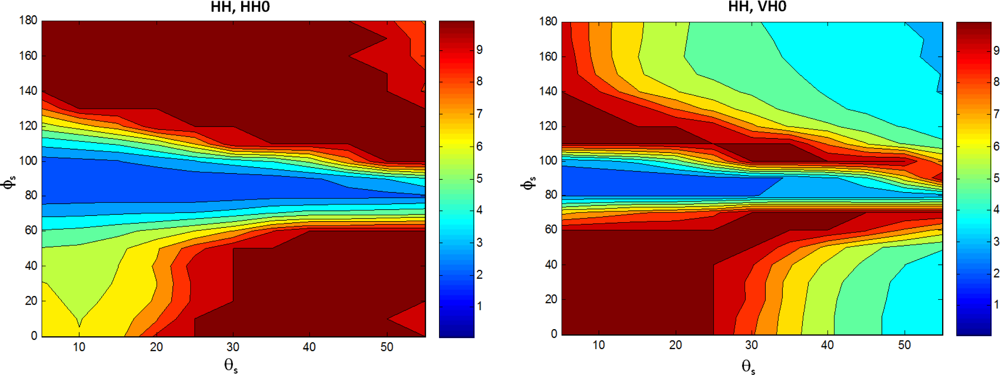
Like in the previous section, the CRLB parameter was estimated, and the maps of the square root of CRLB are here reported, with the same normalization applied in the previous plots. In each figure, two columns are displayed. The left one reports the “co-polarized” CRLB’s, i.e., the CRLB’s calculated assuming that the bistatic and the monostatic measurements have the same polarization (bistatic σ0VV and monostatic σ0VV; bistatic σ0HV and monostatic σ0HV; bistatic σ0HH and monostatic σ0HH). The right column reports the “cross-polarized” CRLB’s, i.e., those calculated for the following couples of measurements: bistatic σ0VV and monostatic σ0HV; bistatic σ0HV and monostatic σ0VV; bistatic σ0HH and monostatic σ0HV. We have verified that the CRLB maps concerning bistatic σ0HV and monostatic σ0VV differ from those concerning bistatic σ0HV and monostatic σ0HH only for their values, but not for what concerns the dependence on the bistatic geometry. For this reason, only one map is reported.
Note that when monostatic σ0HV is available, also a co-polarized measurement is usually carried out, so that two monostatic measurements can be expected to be available from a dual polarization SAR simultaneously with the bistatic one. We have then estimated the CRLB parameter with three measurements too: again, x1 is the corn plant height, h, while the nuisance parameter, x2, has been supposed to be the soil moisture content and the soil roughness has been fixed to σz = 1.5 cm. σ01 is the bistatic measurement, while σ02 and σ03 are the two available measurements in the backscattering direction (e.g., σ0HV and σ0VV or σ0HV and σ0HH). However, it has been found that the addition of another monostatic measurement at L-band (see Equation (5)) does not change the CRLB maps, so that those obtained for the “cross-polarized” CRLBs (shown below) apply for the three measurements case as well. As for the C-band, the addition of the third measurement improves significantly the performance of the retrieval only where the variance is large with two measurements. Nevertheless, the optimal bistatic configurations are obtained at the same azimuth and zenith angles indicated in the case of two measurements. For these reasons, the maps for the three measurements case are not reported.
The maps in Figure 9 indicate that co-polarized and cross-polarized multistatic configurations (left and right column, respectively) behave in the same way. This is partially due to the fact that monostatic σ0HV has been linked to monostatic σ0VV, which, in its turn, is correlated to monostatic σ0HH. Therefore, considering a cross-polarized or a co-polarized backscattering measurement does not change the CRLB maps very much.
At HH and VV polarizations (top and bottom plots), bistatic scattering behaves similarly to backscattering, as long as the azimuth scattering angle φs is far from 90°, and this correlation makes the values of CRLB fairly high on a large range of scattering angles. The maps suggest that the scattering plane orthogonal with respect to the plane of incidence shows the best performance at horizontal polarization, while at vertical polarization, the direction underlined also in the previous sensitivity analysis (see Section 3.1) shows up, that is, φs = 80°, θs = 20° for an incidence direction with θi = 20°. The best achievable value of the variance of the corn height estimate is less than 20 cm, comparable with the one obtained for a purely bistatic configuration and two polarizations. Therefore, the choice between a dual polarized receiver and a receiver at single polarization complemented by a monostatic measurement should be only based on economic considerations (we note that, as for the previous example of Figure 8, the variance of the corn height estimate is larger than 100 cm in the monostatic dual mode).
The maps concerning HV polarization (on the 2nd row) always display large values of CRLB, since the sensitivity of bistatic σ0HV to plant height is rather low outside the plane of incidence (see Figure 5). We remind that the HV backscattering coefficient has been empirically corrected, thus yielding a large CRLB value in the backward direction (i.e., the monostatic configuration), much different from adjacent bistatic configurations in the middle plots of Figures 9 and 10.
If the incidence angle is shifted to higher values, the maps show analogous correlations between measurements, but with slightly higher values of CRLB than in the case of low incidence angle discussed previously. Obviously, the minimum CRLB for the vertical polarization moves towards φs = 70°, θs = 35°, appearing at bistatic directions corresponding to the maximum sensitivity to plant height, as observed in Section 3.1. Moreover, it has been found that, by increasing the cover percentage, CRLB lowers in the specular direction, where the higher coverage produces a higher attenuation and, hence, a higher sensitivity; at other bistatic angles CRLB trend is analogous to the one reported for the reference coverage.
The simulations performed at C-band (Figure 10) indicate that the sensitivity to vegetation biomass in the specular configuration is quite reduced or even absent when the soil roughness is large with respect to wavelength and the percent coverage is low. At C-band, however, when φs is close to 90°, the region with low CRLB gets larger than at the lower frequency, since the vegetation contributions get stronger with respect to the soil ones and the sensitivity to plant height has a smoother trend with bistatic angle. In general, however, the lowest values of CRLB at C-band are higher than the lowest values at L-band.
3.4. Optimal Bistatic Configurations for Crop Height Monitoring
The simulation results presented in the previous sections indicate that the specular configuration (especially at L-band), with a tolerance of about ±5° both in aspect and azimuth, is by far the most sensitive to vegetation biomass. The specular configuration, however, presents some problems in terms of achievable geometrical resolution of a radar imaging system, as discussed in [26]. It becomes very interesting in the case of a GNSS-R system, as discussed, for instance, in [31,41]. Then, it is important to single out other interesting configurations that have emerged from this study.
If the receiver of the bistatic system is foreseen to operate at single polarization (see Figure 5), a low incidence angle (θi∼20°) leads to the best performances. Furthermore, bistatic measurements present sensitivities larger than in the monostatic configuration at vertical polarization with φs = 80°, θs∼θi (at L-band, ΔσVV/Δh can be five-times larger than in backscattering and, at C-band, double) and at horizontal polarization at φs = 90° (where ΔσHH/Δh can be double that in backscattering both at L- and C-band). VV polarization keeps the sensitivity larger in a wider range of bistatic angles with respect to other polarizations, so that, in summary, the best configuration for a receiver with single polarization is:
σ0VV at φs∼80°, θs∼θi
The performance maps developed for the bistatic multipolarization configurations and for the multistatic configurations have shown that several bistatic configurations can provide measurements that are expected to yield good performances. In order to select the most significant ones, we take as a reference the multipolarized measurements performed in monostatic configuration, i.e., the ones, which can be carried out by past and currently available SARs, like ALOS/PALSAR ENVISAT/ASAR, Radarsat or the forthcoming Sentinel 1. We compare the CRLB in this configuration with the ones found in the other scattering directions.
At L-band, the monostatic couples are very much correlated (their CRLB indicates an error standard deviation lower bound always higher than 100 cm, which basically means the inability to measure the height of corn). When two polarizations are available through the passive component of the bistatic system, the scattering angles showing a high sensitivity, mentioned previously, keep their high performances in the combination (σ0VV, σ0HV) and (σ0HH, σ0VH), with a lower bound of the error standard deviation reduced by a factor of about five with respect to the monostatic dual-pol configuration (see Figure 8). When a bistatic measurement is accompanied by a monostatic measurement, the performed simulations (Figure 9) give CRLBs that are much lower than the monostatic values when θi = 20°, with the following multistatic configurations:
σ0VV at φs∼90°, 0 < θs < 20°, together with monostatic σ0VV or σ0HV: this configuration shows the minimum CRLB (i.e., lower bound of the error standard deviation between 15 and 25 cm);
σ0HH at φs∼90°, 0 < θs < 20°, together with monostatic σ0HH or σ0VH (lower bound of the error standard deviation about 25 cm).
At C-band, the error standard deviation is between 50 and 60 cm for the three monostatic couples. Lower values are shown by:
σ0VV at φs∼90°, 0 < θs < 20°, together with monostatic σ0VV or σ0HV (error standard deviation of about 20 cm);
σ0HH at φs∼90°, 0 < θs < 20°, together with monostatic σ0HH or σ0VH (error standard deviation between 20 and 30 cm).
To summarize, the configurations in Table 3 are recommended.
4. Conclusions
In this paper, we have performed an investigation, based on theoretical simulations, on the potential of bistatic and multistatic radar measurements for retrieving crop parameters. To our knowledge, this is the first attempt to analyze this topic. The investigation has taken into account a single crop type (a corn field) and the bistatic configurations, which could be implemented having as master a SAR satellite system operating at one or two polarizations. The results show that, besides the observations around the specular direction, which are implemented, for instance, by the GNSS-R technique, bistatic imaging systems could provide a significant performance in retrieving corn height when looking at about 90° in azimuth with respect to the plane of incidence. The simulations yield a corn height retrieval error standard deviation reduced at least by a factor of three with respect to a monostatic system.
The sensitivity analysis indicates that the most useful responses show up when the soil contribution is at a minimum, so that the vegetation signature shows off with its maximum contrast. Although simulations reported in this paper refer to corn plants, this conclusion may apply to other vegetation types also.
A preliminary analysis of the feasibility of this bistatic geometry, which has been carried out, has shown that the image resolution is still adequate in this geometry, and a limited, but still significant coverage can be ensured using an Envisat type satellite as a master [42]. These results encourage one to further analyze this topic. In particular, the feasibility of the proposed passive radar configuration and an assessment assuming as master a polarimetric SAR should be object of further investigations.
Acknowledgments
The work has been funded by the European Space Agency under contract ESTEC 19173/05/NL/GLC.
References
- Willis, N.J. Bistatic Radar; Artech House: Norwood, MA, USA, 1991. [Google Scholar]
- Griffiths, H.D.; Baker, C.J.; Baubert, J.; Kitchen, N.; Treagust, M. Bistatic Radar Using Satellite-Borne Illuminators. Proceedings of RADAR 2002 (IEE Conference), Edinburgh, UK, 15– 17 October 2002.
- Walterscheid, I.; Ender, J.H.G.; Brenner, A.R.; Loffeld, O. Bistatic SAR processing and experiments. IEEE Trans. Geosci. Remote Sens 2006, 44, 2710–2717. [Google Scholar]
- Lowe, S.T.; LaBrecque, J.L.; Zuffada, C.; Romans, L.J.; Young, L.E.; Hajj, G.A. First spaceborne observation of an earth-reflected GPS signal. Radio Sci 2002, 37, 7-1–7-28. [Google Scholar]
- Gleason, S.; Hodgart, S.; Sun, Y.; Gommenginger, C.; Mackin, S.; Adjrad, M.; Unwin, M. Detection and processing of bistatically reflected GPS signals from Low Earth Orbit for the purpose of ocean remote sensing. IEEE Trans. Geosci. Remote Sens 2005, 43, 1229–1241. [Google Scholar]
- Burkholder, R.J.; Gupta, J.; Johnson, J.T. Comparison of monostatic and bistatic radar images. IEEE Antennas Propag. Mag 2003, 45, 41–50. [Google Scholar]
- Soumekh, M. Moving target detection in foliage using along track monopulse synthetic aperture radar imaging. IEEE Trans. Image Processing 1997, 6, 1148–1163. [Google Scholar]
- Simpson, R.A. Spacecraft studies of planetary surfaces using bistatic radar. IEEE Trans. Geosci. Remote Sens 1993, 31, 465–482. [Google Scholar]
- Martín-Neira, M.; Caparrini, M.; Font-Rossello, J.; Lannelongue, S.; Vallmitjana, C.S. The PARIS concept: An experimental demonstration of sea surface altimetry using GPS Reflected signals. IEEE Trans. Geosci. Remote Sens 2001, 39, 142–150. [Google Scholar]
- Garrison, J.L.; Komjathy, A.; Zavorotny, V.U.; Katzberg, S.J. Wind speed measurement using forward scattered GPS signals. IEEE Trans. Geosci. Remote Sens 2002, 40, 50–65. [Google Scholar]
- Sanz-Marcos, J.; Lopez-Dekker, P.; Mallorqui, J.J.; Aguasca, A.; Prats, P. SABRINA: A SAR bistatic receiver for interferometric applications. IEEE Geosci. Rem. Sens. Lett 2007, 4, 307–311. [Google Scholar]
- Rodriguez-Cassola, M.; Baumgartner, S.V.; Krieger, G.; Moreira, A. Bistatic TerraSAR-X/F-SAR spaceborne-airborne SAR experiment: Description, data processing, and results. IEEE Trans. Geosci. Remote Sens 2010, 48, 781–793. [Google Scholar]
- Krieger, G.; Moreira, A.; Fiedler, H.; Hajnsek, I.; Werner, M.; Younis, M.; Zink, M. TANDEM-X: A satellite formation for high-resolution SAR interferometry. IEEE Trans. Geosci. Remote Sens 2007, 45, 3317–3341. [Google Scholar]
- Rodriguez-Cassola, M.; Prats, P.; Schulze, D.; Tous-Ramon, N.; Steinbrecher, U.; Marotti, L.; Nannini, M.; Younis, M.; Lopez-Dekker, P.; Zink, M.; Reigber, A.; Krieger, G.; Moreira, A. First bistatic spaceborne SAR experiments with TanDEM-X. IEEE Geosci. Rem. Sens. Lett 2012, 9, 33–37. [Google Scholar]
- Engman, E.T.; Chauhan, N.S. Status of microwave soil moisture measurements with remote sensing. Remote Sens. Environ 1995, 51, 189–198. [Google Scholar]
- Wagner, W.; Bloschl, G.; Pampaloni, P.; Calvet, J.C.; Bizzarri, B.; Wigneron, J.P.; Kerr, Y. Operational readiness of microwave remote sensing of soil moisture for hydrology applications. Nord. Hydrol 2007, 38, 1–20. [Google Scholar]
- Pierdicca, N.; Castracane, P.; Pulvirenti, L. Inversion of electromagnetic models for bare soil parameter estimation from multifrequency polarimetric SAR data. Sensors 2008, 8, 8181–8200. [Google Scholar]
- Barrett, B.W.; Dwyer, E.; Whelan, P. Soil moisture retrieval from active spaceborne microwave observations: An evaluation of current techniques. Remote Sens 2009, 1, 210–242. [Google Scholar]
- Pierdicca, N.; Pulvirenti, L.; Bignami, C. Soil moisture estimation over vegetated terrains using multitemporal remote sensing data. Remote Sens. Environ 2010, 114, 440–448. [Google Scholar]
- Della Vecchia, A.; Ferrazzoli, P.; Guerriero, L.; Ninivaggi, L.; Strozzi, T.; Wegmüller, U. Observing and modeling multifrequency scattering of maize during the whole growth cycle. IEEE Trans. Geosci. Remote Sens 2008, 46, 3709–3718. [Google Scholar]
- Notarnicola, C.; Posa, F. Inferring vegetation water content from C- and L-band SAR images. IEEE Trans. Geosci. Remote Sens 2007, 45, 3165–3171. [Google Scholar]
- Engdahl, M.E.; Borgeaud, M.; Rast, M. The use of ERS-1/2 tandem interferometric coherence in the estimation of agricultural crop heights. IEEE Trans. Geosci. Remote Sens 2001, 39, 1799–1806. [Google Scholar]
- Lopez-Sanchez, J.M.; Hajnsek, I.; Ballester-Berman, J.D. First demonstration of agriculture height retrieval with PolInSAR airborne data. IEEE Geosci. Remote Sens. Lett 2012, 9, 242–246. [Google Scholar]
- Katzberg, S.J.; Torres, O.; Grant, M.S.; Masters, D. Utilizing calibrated GPS reflected signals to estimate soil reflectivity and dielectric constant: Results from SMEX02. Remote Sens. Environ 2006, 100, 17–28. [Google Scholar]
- Rodríguez-Álvarez, N.; Camps, A.; Vall-llosera, M.; Bosch-Lluis, X.A.; Monerris, A.; Ramos-Pérez, I.; Valencia, E.; Marchán-Hernandez, J.F.; Martinez-Fernandez, J.; Baroncini-Turicchia, G.; Pérez-Gutiérrez, C.; Sanchez, N. Land geophysical parameters retrieval using the interference pattern GNSS-R technique. IEEE Trans. Geosci. Remote Sens 2011, 49, 71–84. [Google Scholar]
- Pierdicca, N.; Pulvirenti, L.; Ticconi, F.; Brogioni, M. Radar bistatic configurations for soil moisture retrieval: A simulation study. IEEE Trans. Geosci. Remote Sens 2008, 46, 3252–3264. [Google Scholar]
- Pierdicca, N.; De Titta, L.; Pulvirenti, L.; della Pietra, G. Bistatic radar configuration for soil moisture retrieval: Analysis of the spatial coverage. Sensors 2009, 9, 7250–7265. [Google Scholar]
- Ulander, L.M.H.; Frolind, P.; Gustavsson, A.; Stenstrom, G. Bistatic P-Band SAR Signatures of Forests and Vehicles. Proceedings of 2012 IEEE International Geoscience and Remote Sensing Symposium (IGARSS), Munich, Germany, 22– 27 July 2012; pp. 311–314.
- Liang, P.; Pierce, L.; Moghaddam, M. Radiative Transfer model for microwave bistatic scattering from forest canopies. IEEE Trans. Geosci. Remote Sens 2005, 43, 2470–2483. [Google Scholar]
- Ferrazzoli, P.; Guerriero, L.; Solimini, D. Simulating bistatic scatter from surfaces covered with vegetation. J. Electromagnet. Wave. Applicat 2000, 14, 233–248. [Google Scholar]
- Ferrazzoli, P.; Guerriero, L.; Pierdicca, N.; Rahmoune, R. Forest biomass monitoring with GNSS-R: Theoretical simulations. Adv. Space Res 2011, 47, 1823–1832. [Google Scholar]
- Bracaglia, M.; Ferrazzoli, P.; Guerriero, L. A fully polarimetric multiple scattering model for crops. Remote Sens. Environ 1995, 54, 170–179. [Google Scholar]
- Della Vecchia, A.; Ferrazzoli, P.; Guerriero, L.; Blaes, X.; Defourny, P.; Dente, L.; Mattia, F.; Satalino, G.; Strozzi, T.; Wegmüller, U. Influence of geometrical factors on crop backscattering at C-band. IEEE Trans. Geosci. Remote Sens 2006, 44, 778–790. [Google Scholar]
- Ulaby, F.T.; El-Rayes, M.A. Microwave dielectric spectrum of vegetation—Part II: Dual dispersion model. IEEE Trans. Geosci. Remote Sens 1987, 25, 550–556. [Google Scholar]
- Fung, A.K.; Eom, H.J. Coherent scattering of a spherical wave from an irregular surface. IEEE Trans. Antennas Propagat 1983, 31, 68–72. [Google Scholar]
- Fung, A.K. Microwave Scattering and Emission Models and Their Applications; Artech House: Norwood, MA, USA, 1994. [Google Scholar]
- Ferrazzoli, P.; Guerriero, L.; Schiavon, G. Experimental and model investigation on radar classification capabilities. IEEE Trans. Geosci. Remote Sens 1999, 37, 960–968. [Google Scholar]
- Ferrazzoli, P.; Wigneron, J.P.; Guerriero, L.; Chanzy, A. Multifrequency emission of wheat: Modeling and applications. IEEE Trans. Geosci. Remote Sens 2000, 38, 2598–2607. [Google Scholar]
- Ferrazzoli, P.; Guerriero, L. Synergy of Active and Passive Signatures to Decouple Soil and Vegetation Effects. Proceedings of 2010 11th Specialist Meeting On Microwave Radiometry and Remote Sensing of the Environment, Washington, DC, USA, 1– 4 March 2010; pp. 86–89.
- Macelloni, G.; Nesti, G.; Pampaloni, P.; Sigismondi, S.; Tarchi, D.; Lolli, S. Experimental validation of surface scattering and emission models. IEEE Trans. Geosci. Remote Sens 2000, 38, 459–469. [Google Scholar]
- Egido, A.; Caparrini, M.; Ruffini, G.; Paloscia, S.; Santi, E.; Guerriero, L.; Pierdicca, N.; Floury, N. Global navigation satellite systems reflectometry as a remote sensing tool for agriculture. Remote Sens 2012, 4, 2356–2372. [Google Scholar]
- Pierdicca, N.; Pulvirenti, L.; Ticconi, F.; Pampaloni, P.; Macelloni, G.; Brogioni, M.; Pettinato, S.; Guerriero, L.; Ferrazzoli, P.; della Pietra, G.; Capobianco, F. Use of Bi-Static Microwave Measurements for Earth Observation, Final Report ESA CONTRACT No. ESTEC 19173/05/NL/GLC. 2007.
Appendix
A detailed description of the active and passive version of the Tor Vergata model can be found in [A1,A2], respectively. Here, the main steps leading to the refinements developed to simulate the bistatic scattering coefficient of a corn crop will be recalled.
In the scattering models available in the literature, contributions of the various sources of scattering and absorption are combined by using, basically, the Radiative Transfer theory. Nevertheless, this theory can be implemented using different numerical procedures; the Tor Vergata model adopts the Matrix doubling method [A3]. In the corn cover analyzed in this study, three main layers of the canopy have been identified. Predominant scatterers were identified for each one, as it is summarized in the following table:

| Top Layer | Leaves, twigs |
| Middle Layer | Stems |
| Bottom Layer | Soil |
To characterize the behavior of the vegetation medium, the vegetation layers are further subdivided into N elementary sublayers, thin enough to neglect interactions among scatterers within the same elementary layer, and where only single scattering is present. For each sublayer, both the upper and lower half-spaces are subdivided into Nθ discrete intervals of angular amplitude Δθ, both in the incidence θi and scattering θs off-normal angles.
Scattering from each sublayer, for a downwards propagating wave at q polarization (either H or V), is described by an upper half-space scattering matrix S− and by a lower half-space scattering matrix S+. In [A2], it has been demonstrated that the (j,k)-th elements of the scattering matrices are:
In order to correctly include both the scattering effects and the attenuation, a transmission matrix, T, is defined as the sum of the downward scattered specific intensity, S+, and the fraction of forward propagating intensity affected by attenuation [A2]. This is accomplished by adding to the diagonal elements of the matrix, S+pq, a quantity equal to (1 − keq(θij)), where keq(θij) is the fraction of power traveling along the θij direction, at polarization q, which undergoes extinction in the considered sub-layer:
In order to achieve a considerable improvement in the fineness subdivision of the angular directions, without much increase in computation complexity [A3], the scattering and transmission matrices are Fourier transformed with respect to φs − φi. In this way, each elementary layer is characterized by NM pairs of matrices, Sm (previously called S−) and Tm, corresponding to the NM Fourier components through which the azimuthal dependence is expressed.
The contributions of two adjacent thin sublayers are then combined through the Matrix doubling algorithm (Chapter 8 of [36]). For a pair of adjacent sublayers, characterized by matrices, S1m, T1m and S2m, T2m, respectively, the matrices of the combination are given by:
By reiterating this procedure, the N sub-layers are successively combined, and the scattering Smtop and transmission matrices, Tmtop, of the top vegetation layer are computed. We remind that the doubling procedure is applied to each NM matrix, Sm and Tm, and that the elements of the matrices are functions of θi, θs, p and q (Spqm(θi,θs)). In the case of the corn crop canopy, the same procedure is applied to the middle layer of the canopy, so that the whole vegetation layer is obtained applying again the matrix doubling:
The scattering properties of the soil are expressed by the dimensionless bistatic scattering coefficient σ0gpq(θi, θs, φs − φi), which is employed to obtain the Sgpq matrix. Similarly to the matrix of the vegetation elementary layer:
Once the total matrices Stm are computed, the total scattering functions in the direction characterized by the angles φs and θs, which represents the observation angle of the bistatic system, can be obtained by the Fourier series:
References
- Ferrazzoli, P.; Guerriero, L. Radar sensitivity to tree geometry and woody volume: A model analysis. IEEE Trans. Geosci. Remote Sens 1995, 33, 360–371. [Google Scholar]
- Ferrazzoli, P.; Guerriero, L. Passive microwave remote sensing of forests: A model investigation. IEEE Trans. Geosci. Remote Sens 1996, 34, 433–443. [Google Scholar]
- Twomey, S.; Jacobowitz, H.; Howell, H.B. Matrix methods for multiple scattering problems. J. Atmos. Sci 1996, 23, 289–295. [Google Scholar]


| Polarization | Incidence Angle (θi) [deg] | Azimuth Scattering Angle (φs) [deg] | Zenith Scattering Angle (θs) [deg] |
|---|---|---|---|
| HH, VV, HV | 20, 35, 50 | 0 to 180, step 10 | 0 to 60 step 10 |
| Soil Roughness (cm) | Soil Correlation Length (cm) | Soil Moisture Content (%) |
|---|---|---|
| 0.5, 1.5 | 5 (exponential autocorrelation function) | 10, 25 |
| Bistatic σ0VV | Bistatic σ0HH |
|---|---|
| in single configuration | in single configuration |
| combined with bistatic σ0VH | combined with bistatic σ0HV |
| combined with monostatic σ0VV or σ0VH | combined with monostatic σ0HH or σ0HV |
| L-Band | C-Band |
|---|---|
| θi = 20° | θi = 20° |
| φs∼90° ± 5°, | φs∼90° ± 10°, |
| 0 ≤ θs ≤ 20° | θs∼0° |
Share and Cite
Guerriero, L.; Pierdicca, N.; Pulvirenti, L.; Ferrazzoli, P. Use of Satellite Radar Bistatic Measurements for Crop Monitoring: A Simulation Study on Corn Fields. Remote Sens. 2013, 5, 864-890. https://doi.org/10.3390/rs5020864
Guerriero L, Pierdicca N, Pulvirenti L, Ferrazzoli P. Use of Satellite Radar Bistatic Measurements for Crop Monitoring: A Simulation Study on Corn Fields. Remote Sensing. 2013; 5(2):864-890. https://doi.org/10.3390/rs5020864
Chicago/Turabian StyleGuerriero, Leila, Nazzareno Pierdicca, Luca Pulvirenti, and Paolo Ferrazzoli. 2013. "Use of Satellite Radar Bistatic Measurements for Crop Monitoring: A Simulation Study on Corn Fields" Remote Sensing 5, no. 2: 864-890. https://doi.org/10.3390/rs5020864