Chromophoric Dissolved Organic Matter and Dissolved Organic Carbon from Sea-Viewing Wide Field-of-View Sensor (SeaWiFS), Moderate Resolution Imaging Spectroradiometer (MODIS) and MERIS Sensors: Case Study for the Northern Gulf of Mexico

Abstract

Empirical band ratio algorithms for the estimation of colored dissolved organic matter (CDOM) and dissolved organic carbon (DOC) for Sea-viewing Wide Field-of-view Sensor (SeaWiFS), Moderate Resolution Imaging Spectroradiometer (MODIS) and MERIS ocean color sensors were assessed and developed for the northern Gulf of Mexico. Match-ups between in situ measurements of CDOM absorption coefficients at 412 nm (a_CDOM(412)) with that derived from SeaWiFS were examined using two previously reported reflectance band ratio algorithms. Results indicate better performance using the R_rs(510)/R_rs(555) (Bias = −0.045; RMSE = 0.23; SI = 0.49, and R² = 0.66) than the R_rs(490)/R_rs(555) reflectance band ratio algorithm. Further, a comparison of a_CDOM(412) retrievals using the R_rs(488)/R_rs(555) for MODIS and R_rs(510)/R_rs(560) for MERIS reflectance band ratios revealed better CDOM retrievals with MERIS data. Since DOC cannot be measured directly by remote sensors, CDOM as the colored component of DOC is utilized as a proxy to estimate DOC remotely. A seasonal relationship between CDOM and DOC was established for the summer and spring-winter with high correlation for both periods (R²∼0.9). Seasonal band ratio empirical algorithms to estimate DOC were thus developed using the relationships between CDOM-R_rs and seasonal CDOM-DOC for SeaWiFS, MODIS and MERIS. Results of match-up comparisons revealed DOC estimates by both MODIS and MERIS to be relatively more accurate during summer time, while both of them underestimated DOC during spring-winter time. A better DOC estimate from MERIS in comparison to MODIS in spring-winter could be attributed to its similarity with the SeaWiFS band ratio CDOM algorithm.

1. Introduction

Dissolved organic matter (DOM), the largest bioreactive inventory of carbon in the global ocean comparable in size to the atmospheric CO₂ stock has a major impact on the global carbon cycle and climate change [1,2]. The abundance of DOM has generally been determined as dissolved organic carbon (DOC), a major component of organic carbon [3]. Chromophoric DOM (CDOM), the colored component of DOM primarily absorbs light in the UV and visible spectral range affecting the intensity and spectral quality of the light field in the aquatic medium. Because in situ measurement and analysis of DOC is time-consuming and expensive [4,5], the potential for satellite estimates of DOC could provide a useful tool with synoptic and repeated coverage. However, DOC cannot be sensed directly by ocean color sensors; CDOM, the colored fraction of DOC, can be estimated remotely. Thus, CDOM can be utilized as an inexpensive intermediary to estimate the standing stock of DOC and the carbon cycle in aquatic environments. Coble [6] reported CDOM’s contribution to DOC ranged from 20% to 70% in the ocean. The optical signature of CDOM can thus be used as a proxy for DOC as long as these two parameters behave conservatively in the marine environment [7,8]. However, a robust bio-optical algorithm to retrieve CDOM from ocean color sensors must be available [7].

CDOM as well as other photoreactive in-water constituents (e.g., chlorophyll-a, detritus or non-algal particles) affect the underwater light field and the optical properties of water [9,10]. Hence, several ocean color algorithms have been developed to study CDOM distribution both spatially and temporally. Semi-analytical (SA) inversion models have been developed for the Sea-viewing Wide Field-of-view Sensor (SeaWiFS) and Moderate Resolution Imaging Spectroradiometer (MODIS) to derive CDOM and detritus absorption coefficient as a single component (CDM) [11–14], as both exhibit similar spectral shape and slope in the visible light spectrum [15]. In order to investigate carbon cycling in coastal and estuarine waters (Case-2 waters) where optically active constituents often do not co-vary with chlorophyll-a, knowledge of CDOM’s distribution and dynamics is required [16–18]. Empirical algorithms, also known as band ratio algorithms, are based on statistical relationships between R_rs band ratios and the concentration of seawater constituents [18–23]. For example, Kahru and Mitchell [19] developed a relationship between a_CDOM(300) and SeaWiFS R_rs(443)/R_rs(510) at the CalCOFI site in southern California. D’Sa and Miller [20] developed an algorithm to retrieve a_CDOM(412) from ocean color data in the Mississippi River dominated coastal waters using a relationship between a_CDOM(412) and the SeaWiFS reflectance band ratio of R_rs(510)/R_rs(555). For the coastal waters adjacent to the Chesapeake and Delaware Bays, Johannessen et al.[21] reported the relationship between ultraviolet (UV) attenuation coefficient (K_d) at 323 nm, 338 nm, and 380 nm and the R_rs(412)/R_rs(555) band ratio. Recently, Zhu et al.[24] developed an Extended Quasi-Analytical Algorithm (QAA-E) to estimate CDOM in the Mississippi and Atchafalaya River plume regions using above-surface hyper-spectral light measurements.

Conservative behavior between CDOM absorption coefficient and DOC has been reported in different types of water bodies [8,25–28]. CDOM absorption coefficient (a_CDOM(λ)) and DOC concentration are highly correlated with each other in regions where the mixing of fresh and oceanic waters control the variability of each parameter and terrestrial dominance is strong [29]. These conditions have enabled satellite estimates of DOC using the relationship between CDOM-DOC and CDOM-R_rs band ratios [7,22]. Mannino et al.[22] developed algorithms to derive DOC through the relationship between the a_CDOM at 412 nm, 355 nm, DOC, and R_rs ratios for MODIS/Aqua and SeaWiFS in coastal waters of the US Middle Atlantic Bight. Del Castillo and Miller [7] applied the R_rs(510)/R_rs(670) band ratio to SeaWiFS imagery to retrieve DOC in the Mississippi River plume. The high rates of water discharge containing elevated levels of DOC and CDOM by the Mississippi and Atchafalaya Rivers into the coastal waters strongly impacts the biogeochemical processes and fluxes in the northern Gulf of Mexico. Satellite ocean color remote sensing offers the capability to monitor CDOM and DOC distribution spatially and temporally and to improve understanding of the carbon cycling in this large river delta-front estuary (LDE) [30].

The primary goal of this study is to evaluate existing and to develop new ocean color algorithms for CDOM absorption and DOC concentrations in the northern Gulf of Mexico. An extended set of field CDOM absorption and DOC measurements collated for the northern Gulf of Mexico as part of a NASA funded project were used in this study. Algorithm assessment and development were based on two empirical band ratio CDOM algorithms, namely the D’Sa et al.[18] and the Mannino et al.[22] algorithms for estimating a_CDOM(412). These algorithms were extended to MODIS/Aqua and the MERIS/ENVISAT sensors. Further, DOC empirical algorithms were developed through the relationships between in situ a_CDOM(412)-in situ DOC and in situ a_CDOM(412)-R_rs band ratios (satellite-derived) (e.g., Mannino et al.[22]). This approach was found to be an effective method to derive DOC concentration. The satellite-derived DOC concentration enabled us to monitor DOC variations both spatially and temporally, and to enhance our understanding of the organic carbon processes in this LDE in the northern Gulf of Mexico.

2. Materials and Methods

2.1. Study Area

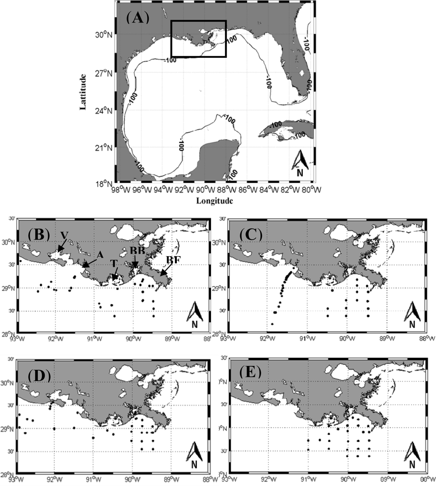
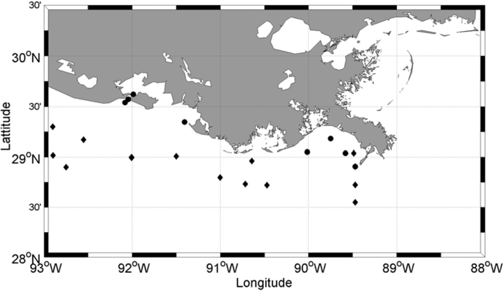
The study area is located in the northern Gulf of Mexico on the Texas-Louisiana shelf, covering the region from latitude 28.0° to 30.5°N and longitude 88.0° to 93.0°W (Figure 1(A)). The study site is highly influenced by the discharge from the Mississippi River (MR) and its largest distributary, the Atchafalaya River (AR). The Mississippi River drains approximately 41% of the contiguous United States, making it the third largest drainage basin in the world. The MR also ranks as the seventh largest river in terms of fresh water discharge [31,32]. The Mississippi-Atchafalaya River System (MARS) discharges ∼70% of its total flow into the Gulf of Mexico through the MR Birdfoot delta while the remainder discharges through the AR and Wax Lake outlets into the broad, shallow Atchafalaya bay [33,34]. Seasonal variations and the large discharge of freshwater from the MR and AR profoundly influence the bio-optical properties of water, primary productivity, and the distribution of carbon flux in the region [20,34–37]. Terrestrially-derived (riverine or allochthonous) CDOM introduced by the MR and AR predominates the northern Gulf of Mexico [38]. The annual export of DOC from the Mississippi and the Atchafalaya Rivers into the Gulf of Mexico was reported 1.75 Tg and 0.95 Tg, respectively. These amounts account for about 0.8%–1.1% of the total global input of DOC from rivers to the ocean [39].

2.2. Field Sampling

Field data comprising of CDOM optical (spectral absorption coefficient) and DOC concentrations in conjunction with physical (salinity) properties of water were obtained from the study area during 17 oceanographic cruises in 2005 and 2007–2009 (

Table 1. Field data from cruises in the northern Gulf of Mexico along with mean values for a_CDOM(412), dissolved organic carbon (DOC) concentration, salinity, and S.D., and Geometric mean for each cruise.

Cruise	Date	aCDOM(412) (m−1)	DOC (μmol·C·L−1)	Salinity (psu)	S.D.aCDOM(412)	Geometric MeanaCDOM(412)
1	23–29 March2005	0.47	n/a	27.07	0.22	0.43
2	20–25 May 2005	0.43	n/a	27.07	0.16	0.39
3	8–12 July 2005	0.23	n/a	29.27	0.18	0.17
4	18–24 August 2005	0.25	n/a	28.75	0.13	0.22
5	23–28 March 2007	n/a	204.51	n/a	-	-
6	16–20 April 2007	2.79	n/a	31.75	2.09	1.62
7	7–10 May 2007	0.87	180.02	24.16	0.93	0.33
8	17 and 19 July 2007	1.43	288.23	15.12	0.60	1.34
9	17–20 July 2007	n/a	155.13	n/a	-	-
10	9 August 2007	0.74	266.58	27.64	0.20	0.73
11	11 and 13 September 2007	1.97	509.74	11.33	0.44	1.93
12	9–12 February 2008	1.72	361.68	11.28	0.58	1.64
13	5–8 April 2008	3.72	664.30	2.60	1.35	3.49
14	6–8 April 2008	0.82	n/a	22.33	0.56	0.55
15	6–18 April 2008	n/a	226.69	n/a	-	-
16	2 June 2008	2.52	377.25	11.23	0.19	2.51
17	18–20 August 2009	0.34	166.97	27.94	0.27	0.22

; Figure 1). Some of the field data from these cruises were hosted as part of a NASA funded project by the Biological and Chemical Oceanography Data Management Office (BCO-DMO) as a data rescue effort. In the spring and summer (March, May, July, and August) of 2005, coastal waters influenced by the MR from Southwest Pass to the Atchafalaya Delta were sampled aboard the RV Gyre. Water samples were collected from the surface using Niskin bottles attached to the conductivity-temperature-depth (CTD) profiler (Sea-Bird Electronic, Inc., Bellevue, WA, USA). The samples were filtered through pre-rinsed 0.2 μm Nuclepore membrane filters within three hours of collection. Spectral absorption of filtered samples was obtained onboard the ship using a single-beam spectrophotometer [40]. Water samples taken in April 2007 were collected and analyzed similar to the samples taken in 2005. Field samples collected in May 2007 in the AR plume region onboard RV Pelican were obtained from the Biological and Chemical Oceanography Data Management Office (BCO-DMO) website ( http://data.bco-dmo.org/jg/serv/BCO/NACP_Coastal/GulfMexico), samples were filtered through 0.2 μm Polyether sulfone filters into baked (550 °C; 5 h minimum) collection vials and stored at 4 °C in the dark until processed in the laboratory. More information can be found on the BCO-DMO website.

In situ data obtained during the 2007 (July, August, September) and 2008 (February, April, June) cruises were also used. Near-shore sampling was conducted from a small boat in transects out of the Vermilion, Atchafalaya, Terrebonne, and Barataria Bays, and the Mississippi River’s Southwest Pass. Discrete water samples were collected 0.5 m below the water surface using a Sea-Bird 25 CTD. Water samples were filtered through Whatman 47 mm GF/F filters, nominal pore size 0.7 μm, into combusted glass flasks for CDOM and DOC analysis [41]. DOC measurements were obtained during cruises onboard the RV Pelican in March and July of 2007 and April and July of 2008 as part of the Mechanisms Controlling Hypoxia (MCH) project. In August 2009, in situ observations were made onboard the RV Pelican on the Louisiana continental shelf. In situ samples from the water surface were collected using Niskin bottles attached to CTD profiles. Samples were immediately filtered under low vacuum through a Whatman GF/F filter (nominal pore size 0.2 μm) and then stored in pre-cleaned amber glass bottles and refrigerated until CDOM absorption and DOC concentration were measured in the laboratory.

2.3. CDOM Absorption

Spectral CDOM absorption values from filtered water obtained in 2005 were determined onboard the ship using a capillary waveguide system (WPI, Inc., Sarasota, FL, USA), a single-beam spectrophotometer [42,43]. The optical absorbance spectra (A) were obtained between 250 nm to 722 nm from two scans, namely, a cell filled with blank solution (Milli-Q water), adjusted for the sample salinity followed by a water sample scan. The absorbance values at each wavelength were corrected for baseline fluctuation and scattering by subtracting the absorbance averaged between 715 to 722 nm [40]. The absorption coefficients at each wavelength (a_CDOM(λ)) (m⁻¹) were calculated using the following equation:

$$a\left(\lambda \right)=\frac{2.303A\left(\lambda \right)}{l}$$

(1)

where l, the optical path length (m) used for the absorbance measurements were 0.1 or 0.5 m [40].

CDOM absorption from filtered water samples obtained during 2007 (July, August, September) and 2008 (February, April, June) were obtained with a Shimadzu UV1700 dual-beam spectrophotometer using a 1-cm cuvette at 1 nm intervals between 350–700 nm. Spectra were then normalized by subtracting each wavelength from the measured value at 700 nm [41]. The CDOM absorption measurement method used to analyze the May 2007 water samples is documented at BCO-DMO website ( http://data.bco-dmo.org/jg/serv/BCO/NACP_Coastal/GulfMexico/CDOM.html0). Filtered samples from the August 2009 survey were processed in the laboratory on a double beam Perkin Elmer Lambda 850 spectrophotometer between 190 to 750 nm at 2 nm intervals. Samples were brought to room temperature before measuring the absorbance spectra of CDOM. Before determining a_CDOM(λ), absorbance data were corrected by subtracting the mean absorbance from 700 to 750 nm from each wavelength. The CDOM absorption coefficient at each wavelength was derived using Equation (1).

2.4. DOC Concentration

The DOC concentration of filtered-water samples obtained in 2007 (July, August, September) and in 2008 (February, April, June) was measured using a Shimadzu TOC–VCSN analyzer, calibrated with potassium biphthalate [41]. Samples collected in 2007 (March, July) and 2008 (April, July) were filtered through GF/F filters and then acidified (100 μL of 2 N HCl was added in order to remove inorganic carbon). The DOC concentration was then measured with the Shimadzu TOC-VCSH/CSN by using high-temperature catalytic oxidation (HTCO). The DOC concentrations used for this study from the May 2007 cruise were measured by wet chemical oxidation with an OI Analytical Model 1010 TOC analyzer [44]. For the August 2009 samples, DOC concentrations were obtained using a Shimadzu TOC-5000A (with ASI-5000A auto-sampler) using a high temperature combustion method.

2.5. Satellite Data

Satellite data from the SeaWiFS, MODIS, and MERIS sensors were used to evaluate and parameterize CDOM and DOC empirical algorithms using R_rs visible bands; specifically, the performance of two empirical algorithms, namely the D’Sa et al.[18] algorithm using the R_rs(510)/R_rs(555) band ratio and the Maninno et al.[22] algorithm using the R_rs(490)/R_rs(555) band ratios were used to derive a_CDOM(412). Level 1A SeaWiFS LAC (local area coverage) data with spatial resolution of 1.1 km at nadir, and with daily temporal resolution were acquired from NASA Goddard Space Flight Center ( http://oceancolor.gsfc.nasa.gov/). Level 1A data were processed up to Level 2 (L2) using the SeaWiFS Data Analysis System (SeaDAS) developed by NASA’s Ocean Biology Processing Group (OBPG) version 6.0 and IDL 6.3 to derive R_rs bands at 490, 510 and 555 nm. As the field data set spanned the period corresponding to the operational period of three ocean color sensors, the empirical algorithms were evaluated for SeaWiFS as well as the MODIS/Aqua and MERIS/ENVISAT sensors. MODIS/Aqua Level 1A LAC (∼1 km at nadir, daily temporal resolution) were obtained from the NASA’s Ocean Color website and processed to Level 2 (L2) to retrieve R_rs bands at 488 nm and 555 nm using SeaDAS 6.0 software package. The atmospheric correction algorithm developed by Gordon and Wang [45] was used for SeaWiFS and MODIS to derive R_rs bands. Furthermore, R_rs bands using 1 × 1 and 3 × 3 pixel box size (1km/pixel at nadir) centered on the position of field measurements were chosen. Due to paucity of data points, a time window of ±14 h between satellite match-ups and field sampling was set. R_rs bands extracted from a 5 × 5 pixel box for both SeaWiFS and MODIS were also examined, but this pixel box size was not used because of the spatial heterogeneity in coastal waters; therefore, a 3 × 3 pixel box was applied for extracting most data. In order to develop an empirical algorithm to retrieve CDOM and DOC with MERIS/ENVISAT (European Space Agency (ESA)), Level 1 reduced resolution (RR) data, with a spatial resolution of ∼1.2 km and daily temporal resolution, were obtained from ESA ( http://merci-srv.eo.esa.int/merci/welcome.do) and processed to Level 2 using SeaDAS 6.0 software package. R_rs bands at 510 nm and 560 nm were extracted from 1 × 1 and 3 × 3 pixel box size (1.2 km/pixel at nadir) with ±14 h temporal window between satellite overpass and the time of field sampling for obtaining sufficient data points. Matchup comparisons between satellite derived estimates and in situ measurements of CDOM absorption and DOC concentrations were assessed using statistical criteria such as bias, root mean square error, scatter index and the coefficient of determination (

Table 2. Equations used for calculating error statistics for evaluation of algorithms.

Statistical Estimator	Formula
Bias	$$\frac{1}{N}\sum _{i=1}^N\left(y_i-x_i\right)$$
Root mean square error	$$\sqrt{\frac{1}{N}\sum _{i=1}^N{\left(y_i-x_i\right)}^2}$$
Scatter-index	$$\frac{1}{\overline{x}}\sqrt{\frac{1}{N}\sum _{i=1}^N{\left[\left(y_i-\overline{y}\right)-\left(x_i-\overline{x}\right)\right]}^2}$$

where y_i is satellite-derived values and x_i is field-measured values.

).

3. Results

3.1. CDOM, DOC and Salinity Relationships

In order to develop an empirical ocean color DOC algorithm using CDOM’s optical signature as a proxy for DOC, the relationship between these two parameters was examined seasonally (i.e., for summer and spring-winter periods) (

Table 3. Coefficients resulting from regression analysis between a_CDOM(412), DOC, and salinity.

Parameter	Season	Slope (a)	Intercept (b)	R2	N
DOC vs. aCDOM (412)	Summer	137.22	124.20	0.90	39
DOC vs. aCDOM (412)	Spring-winter	127.02	77.97	0.90	40
aCDOM(412) vs. salinity	Summer	−0.079	2.62	0.77	39
aCDOM(412) vs. salinity	Spring-winter	−0.076	2.78	0.86	40
DOC vs. salinity	Summer	−11.48	497.82	0.77	39
DOC vs. salinity	Spring-winter	−11.84	482.64	0.90	40

Linear equations were fitted to all variables (y = a × x + b). In the DOC-CDOM relationship, y = DOC and x = a_CDOM(412); in the CDOM-salinity relationship, y = a_CDOM(412) and x = salinity; in the DOC-salinity relationship, y = DOC and x = salinity. All presented values are within interval Mean ± 1 Stdev.

). Based on the location of the field measurements, the MR discharge strongly influenced the relationships between DOC, CDOM and salinity during summer (August 2007, September 2007, August 2009), while spring-winter data (May 2007, February 2008) were significantly affected by the AR discharge. In summer, a_CDOM(412), DOC concentration and salinity in surface waters ranged from 0.023 to 2.45 m⁻¹ (S.D. = 0.66, geometric mean = 0.35, n = 40), 117 to 488 μmol·C·L⁻¹ (214 ± 95 μmol·C·L⁻¹, n = 40), and 4.39 to 34.39 psu (mean = 24.67 ± 7.30 psu), respectively. During spring-winter study period, a_CDOM(412) varied from 0.011 m⁻¹ to 5.47 m⁻¹ (S.D. = 1.38, geometric mean = 0.52; n = 40), the DOC concentration ranged from 56 to 739 μmol·C·L⁻¹ (246 ± 185 μmol·C·L⁻¹; n = 40), and salinity exhibited a range from 0.43 to 35.9 psu (mean = 23.01 ± 12.21 psu, n = 40). Elevated values of DOC and CDOM observed in spring-winter period were likely due to out-welled CDOM-laden water from productive wetlands adjacent to the AR plume [46].

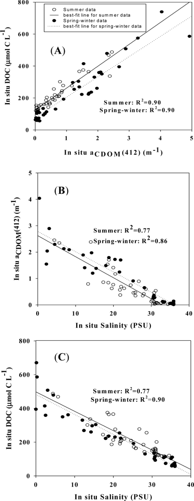
DOC concentrations were regressed against a_CDOM(412) for spring-winter and summer periods to assess the seasonal relationship between DOC and CDOM. Results indicated strong conservative behavior between the two properties for both seasons (Equations (2) and (3); Figure 2(A)), respectively). Regression analyses between a_CDOM(412) and DOC concentration indicated high R² values (0.9) for both seasons with the intercept for the summer relationship (Equation (3)) being higher than that of spring-winter relationship (Equation (2)) (see Table 3).

$$\mathit{DOC}\left(\mu \mathit{mol}\hspace{0.17em}C\hspace{0.17em}{L}^{-1}\right)=127.027\hspace{0.17em}{a}_{CDOM}\left(412\right)+77.97$$

(2)

$$\mathit{DOC}\left(\mu \mathit{mol}\hspace{0.17em}C\hspace{0.17em}{L}^{-1}\right)=137.22\hspace{0.17em}{a}_{CDOM}\left(412\right)+124.20$$

(3)

The high positive correlation between a_CDOM(412) and DOC concentration suggests that these two properties behaved conservatively for the two time periods with mixing between the river and marine end members playing a critical role in the distribution of both CDOM and DOC. The seasonal relationships between a_CDOM(412) and salinity (Table 3; Figure 2(B)) as well as between DOC concentration and salinity (Table 3; Figure 2(C)) exhibited strong linear inverse correlations for the summer and spring-winter periods. The inverse linear correlation between a_CDOM(412) and salinity (R² = 0.77 in summer; R² = 0.86 in spring-winter) suggests strong river-derived or terrestrial sources; however, high CDOM and DOC concentrations due to riverine influences could be masking advective or autochthonous sources (e.g., in situ primary production) or removal processes (e.g., photooxidation, flocculation and sorption). These results indicate similar trends and consistency of a conservative behavior between CDOM and salinity in the northern Gulf of Mexico [40]. The seasonal variation in MR and AR discharges along with effects of mixing caused by energetic atmospheric events (i.e., intrusion of cold fronts or storms) likely induces variability in CDOM optical properties and DOC concentration in the northern Gulf of Mexico [46–48] affecting biogeochemical cycles and the relationship between these two properties and salinity.

A strong negative correlation (Table 3; Figure 2(C)) exhibited between DOC and salinity indicates that terrestrial-derived DOC was conserved during the mixing of river and marine end member waters. The strong correlations between these three properties show the persistent influence of the MR and AR discharges on the CDOM distribution and geochemical cycle in the northern Gulf of Mexico (Coble, 2007). These results indicate that the first condition to derive DOC remotely and exclusively was met here (Figure 2).

Table 4. Station locations, a_CDOM(412), DOC, and salinity data used in Figure 2.

Date	Latitude	Longitude	CDOM	DOC	Salinity
Jul-2007	29.57	−92.04	1.536	375.00	18.47
	29.54	−92.08	1.409	365.83	19.97
	29.62	−91.99	0.792	301.50	13.30
	29.32	−89.94	1.172	276.17	20.49
Aug-2007	29.35	−89.91	0.894	277.42	26.72
	29.32	−89.94	0.597	255.75	28.57
Sep-2007	29.62	−91.99	2.450	487.50	4.39
	29.57	−92.04	2.345	468.58	5.71
	29.35	−89.91	1.706	364.33	18.81
Jun-2008	29.32	−89.94	2.381	336.67	14.02
Sep-2009	29.05	−90.02	0.692	208.83	22.03
	28.38	−89.47	0.083	123.42	31.48
	29.04	−89.49	0.624	186.58	19.56
	29.23	−89.88	0.470	163.00	25.77
	28.87	−90.48	0.173	156.42	30.27
	28.73	−91.00	0.348	185.08	27.76
	28.91	−90.02	0.537	201.00	31.16
	28.55	−89.47	0.051	142.75	30.95
	28.91	−89.47	0.747	209.17	24.58
	29.18	−90.02	0.840	233.75	18.65
	28.72	−90.47	0.459	162.42	30.77
	28.71	−90.00	0.282	159.42	30.90
	28.55	−89.75	0.035	153.17	30.92
	28.91	−89.61	0.373	203.08	21.80
	29.05	−90.02	0.628	219.17	22.84
	28.55	−90.48	0.093	117.17	33.14
	28.53	−90.02	0.042	137.67	30.51
	28.72	−89.75	0.100	130.42	30.80
	28.93	−90.02	0.130	149.08	30.01
	28.38	−90.48	0.060	117.75	32.52
	28.72	−89.47	0.456	171.33	25.29
	29.05	−89.75	0.085	126.25	31.25
	28.98	−90.25	0.567	190.58	21.71
	28.73	−90.72	0.346	163.58	25.83
	28.38	−89.75	0.061	122.25	31.66
	28.91	−89.47	0.767	212.17	19.95
	29.18	−89.75	0.419	142.08	28.02
	29.04	−90.48	0.859	244.50	17.33
	28.53	−91.00	0.023	120.25	34.39

represents the data used in the Figure 2. The data utilized to examine conservative behavior of DOC and CDOM were not used to evaluate and develop empirical algorithms in the following sections.

3.2. CDOM and DOC Empirical Algorithms: Validation and Development

3.2.1. Validation of Empirical Algorithms to Derive CDOM and DOC

The second condition for estimating DOC concentration using satellite ocean color sensors is to provide a robust relationship between R_rs band ratio and CDOM absorption coefficient to retrieve CDOM remotely. Then DOC concentration can be derived through this relationship and the CDOM-DOC relationship. The D’Sa et al.[18] SeaWiFS empirical algorithm developed using the relationship between in situ a_CDOM(412) measurements and reflectance ratios during three field cruises in spring and fall of 2000 and March 2002 in the northern Gulf of Mexico was:

$$a_{\mathit{CDOM}}\left(412\right)=0.277{\left[(R_{rs}\left(510\right)/(R_{rs}\left(555\right)\right]}^{-2.022}$$

(4)

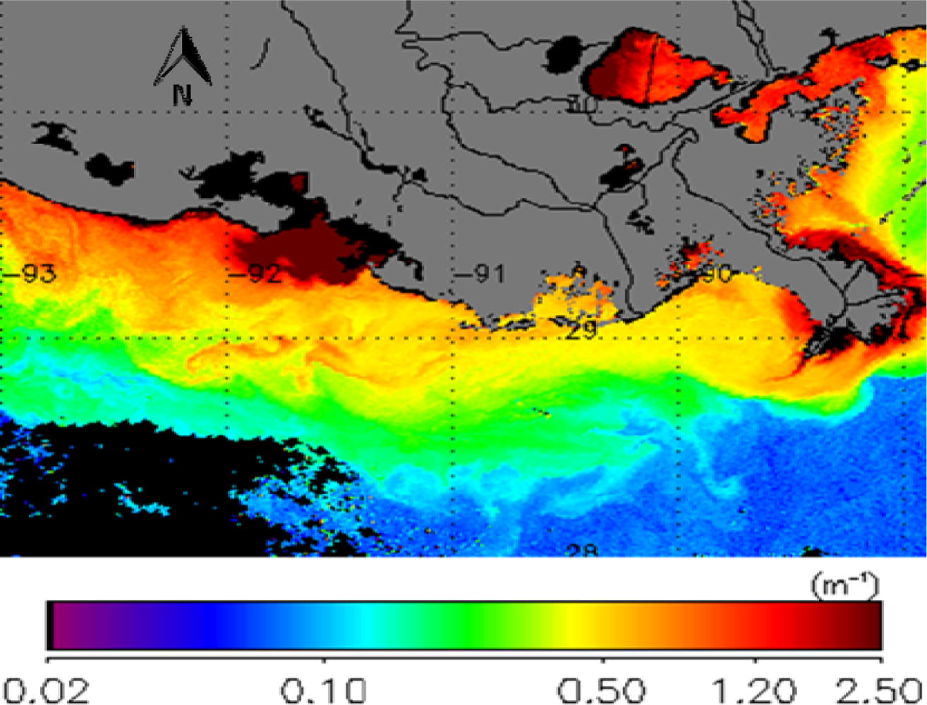
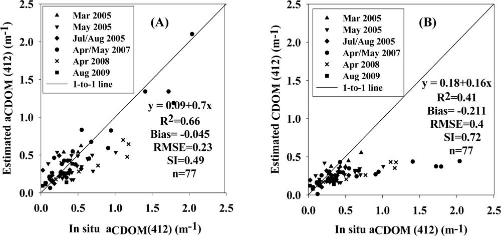
Equation (4) was applied to SeaWiFS data to obtain surface a_CDOM(412) map for 6 February 2007 (Figure 3). The robustness of this algorithm was assessed by comparing satellite-estimated a_CDOM(412) with in situ a_CDOM(412) within ±14 h of the satellite overpass. Match-up comparison illustrates a satisfactory trend and close agreement between satellite-derived and in situ a_CDOM(412) for the study region (Figure 4(A)) with data being uniformly distributed along the one-to-one line. The algorithm was further quantified using bias function, root mean square error (RMSE), scatter-index (SI) and coefficient of determination (R²) (Table 2). The statistical analysis revealed that the D’Sa et al.[18] algorithm performed well in the study area with relatively high R² (0.66), low RMSE (0.23), and low Bias (−0.045) (

Table 5. Summary of error statistics derived from matchup comparisons between in situ and satellite-derived a_CDOM(412) obtained from D’Sa et al.[18] and LM algorithms.

Rrs Band Ratio	R2	RMSE	Bias	SI	Slope	Intercept	N*
Rrs510/Rrs555-D’Sa et al.(2006) algorithm	0.66	0.23	−0.045	0.49	0.70	0.09	77
Rrs490/Rrs555-LM algorithm	0.41	0.40	−0.211	0.72	0.16	0.18	77

^*N is the number of matchup observations.

). The other empirical algorithm assessed was the algorithm which was constructed by localizing the Mannino et al. (2008) [22] algorithm developed to retrieve a_CDOM(412) from SeaWiFS in the US Middle Atlantic Bight. We localized the Mannino et al.[22] algorithm (hereafter, LM, which stands for the localized Mannino et al. (2008) algorithm) with regional data by constructing the relationship between satellite-derived R_rs band ratio (R_rs490/R_rs555) and in situ a_CDOM(412) sampled in the northern Gulf of Mexico. The new relationship was applied to SeaWiFS imagery using SeaDAS 6.0 software to derive a_CDOM(412). To validate the relationship, in situ a_CDOM(412) values were compared with satellite-derived a_CDOM(412) values within ±14 h of the satellite overpass. This yielded R² = 0.41, RMSE = 0.4, and Bias = −0.21 (Table 5; Figure 4(B)). The in situ a_CDOM(412) data used for matchup analysis were independent from the data utilized in the construction of the (R_rs490/R_rs555)-a_CDOM (412) relationship, and were similar to the data used in the D’Sa et al.[18] algorithm validation analysis. The matchup comparison results (Table 5; Figure 4(A,B)) indicate that the performance of an empirical algorithm utilizing R_rs(490)/R_rs(555) for estimation of a_CDOM(412) was less satisfactory than the D’Sa et al.[18] algorithm for the sample data used.

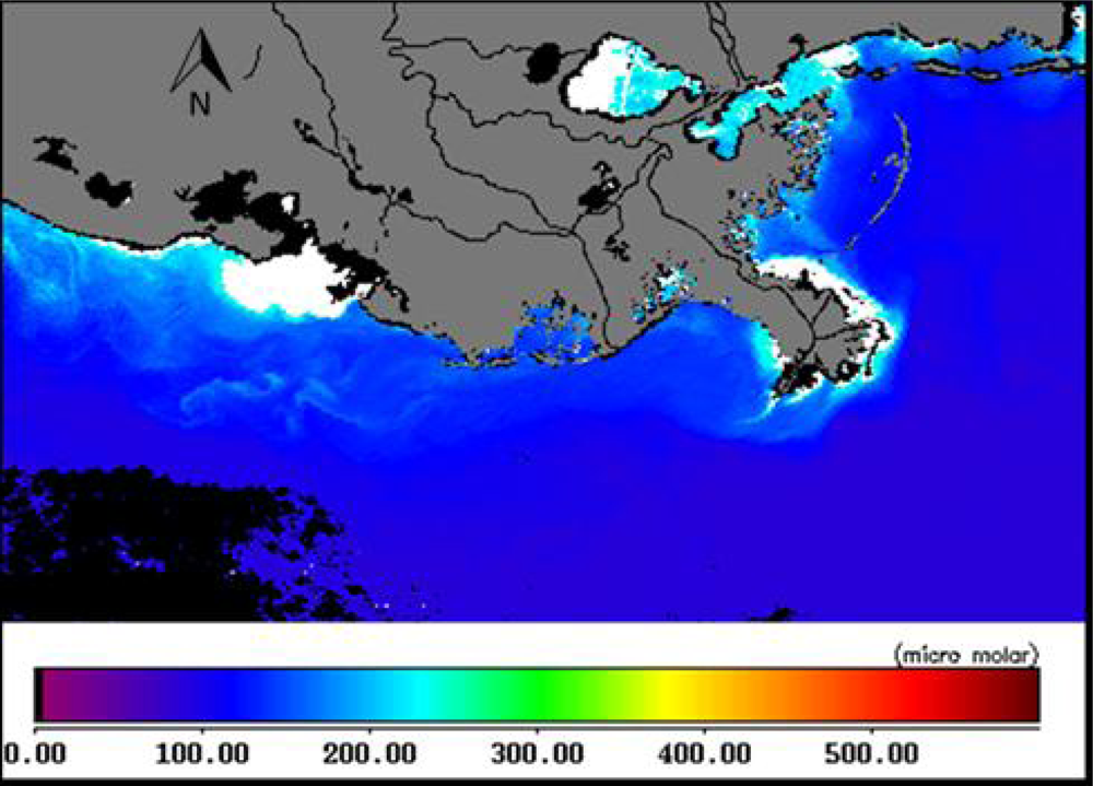
Since the D’Sa et al.[18] SeaWiFS CDOM algorithm was found to be more robust for the estimation of a_CDOM(412) in the northern Gulf of Mexico, this algorithm along with the CDOM-DOC relationship was used to derive DOC concentration remotely. The seasonal DOC algorithms were developed simply through the CDOM-DOC seasonal relationships (Equations (2) and (3)) and the D’Sa et al.[18] algorithm (Equation (4)). The DOC algorithms for the spring-winter and summer are:

$$\mathit{DOC}=28.835{\left[R_{rs}\left(510\right)/(R_{rs}\left(555\right)\right]}^{-2.022}+77.97$$

(5)

$$\mathit{DOC}=31.148{\left[(R_{rs}\left(510\right)/(R_{rs}\left(555\right)\right]}^{-2.022}+124.20$$

(6)

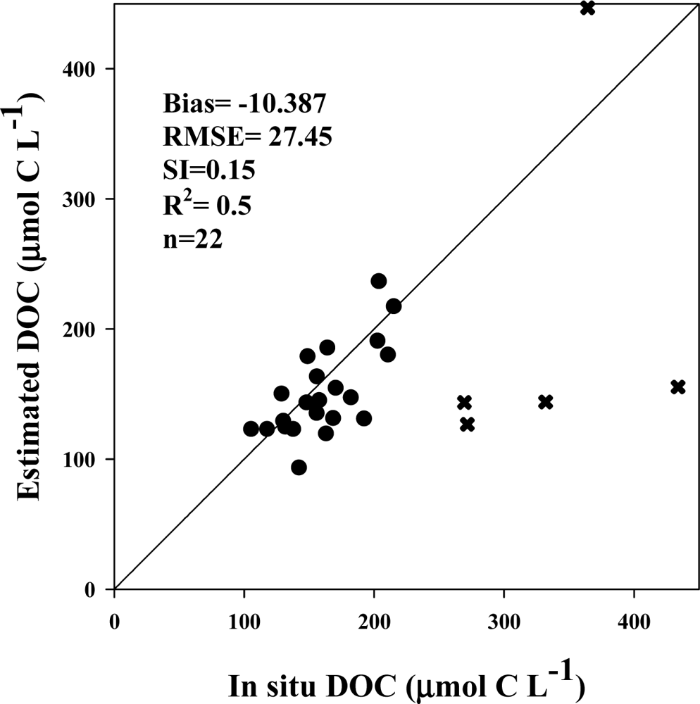
These algorithms were applied to SeaWiFS data to generate surface DOC concentration map (Figure 5). The performance of the newly developed DOC algorithm was examined just for the spring-winter period (Figure 6) due to the paucity of satellite-derived R_rs data in summer. The results of the statistical analysis indicate that retrieval of DOC concentration (μmol·C·L⁻¹) was reasonable (Bias = −10.38, RMSE = 27.45, SI = 0.15, R² = 0.5, and N = 22). Surface DOC concentration obtained remotely using the DOC algorithm (Equation (5)) indicated a 7% percentage difference between SeaWiFS-estimated DOC and field DOC for spring-winter period. However, algorithm performance was found to degrade at elevated DOC concentrations (>250 μmol·C·L⁻¹) and in shallower nearshore and river plume waters.

3.2.2. CDOM and DOC Empirical Algorithms for MODIS and MERIS Sensors

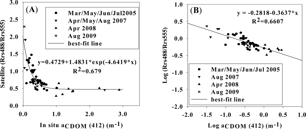
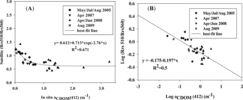
R_rs values at visible bands were derived from MODIS and MERIS to use as inputs to the empirical algorithms for CDOM and DOC. The R_rs band ratios used were R_rs(488)/R_rs(555) for MODIS-Aqua and R_rs(510)/R_rs(560) for MERIS-Envisat with wavebands chosen similar to the D’Sa et al.[18] and Mannino et al.[22]. The band ratio algorithms were regressed against coincident in situ a_CDOM(412) measured within ±14 time difference for MODIS and MERIS overpasses. Non-linear three-parameter exponential decay curves (R² = 0.68 for MODIS, R² = 0.67 for MERIS) (Figures 7(A) and 8(A)) exhibited higher correlation than the log-transformed R_rs band ratios plotted against log-transformed values of in situ a_CDOM(412) (R² = 0.66 for MODIS, R² = 0.5 for MERIS) (Figures 7(B) and 8(B)). CDOM absorption coefficient can thus be retrieved using the R_rs band ratios:

$$a_{\mathit{CDOM}}\left(412\right)=\text{ln}\left[\left(R_{rs}\hspace{0.17em}\mathit{ratio}-A\right)/B\right]/\left(-C\right)$$

(7)

Table 6. Summary of fitted coefficients for the regional MODIS and MERIS empirical algorithm illustrated in Figures 7 and 8 for CDOM and DOC retrievals. Presented coefficients are fitted into the seasonal DOC algorithm.

Product	Satellite	Fitting Curve	Rrs Band Ratio	A	B	C	R2
aCDOM(412)	MODIS	3 parameter exponential decay	488/555	0.472	1.48	4.64	0.67
aCDOM(412)	MERIS	3 parameter exponential decay	510/560	0.612	0.713	2.76	0.67

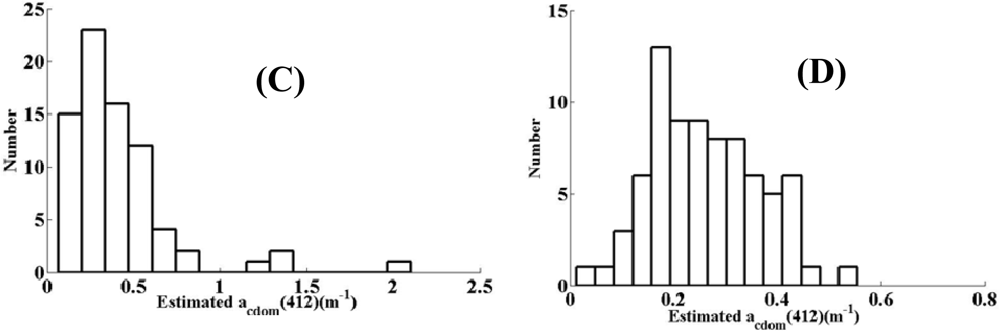
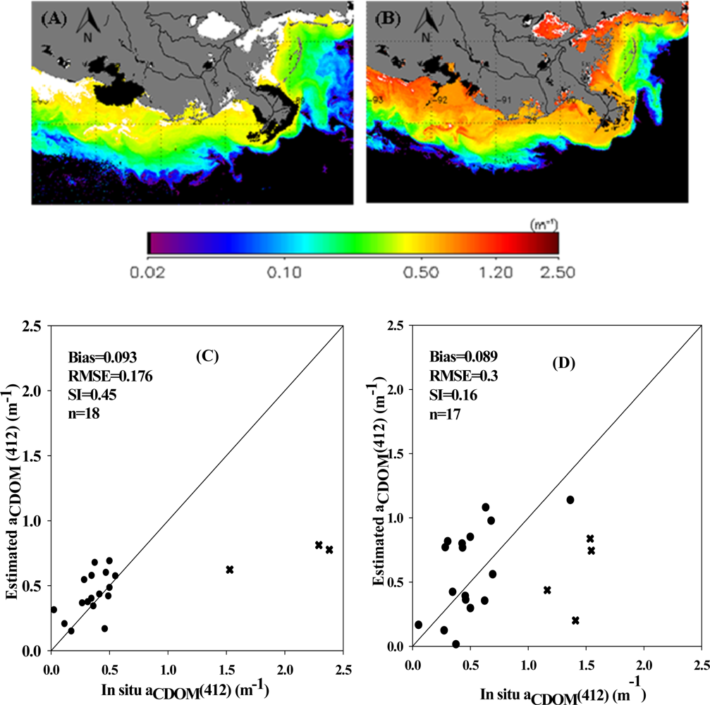
presents R_rs ratio and coefficient values (A, B, and C) for MODIS and MERIS. The regional CDOM empirical algorithms were applied to MODIS and MERIS data (Figure 9(A,B)) to obtain surface CDOM absorption maps. The black regions in the CDOM images could be due to failure of the atmospheric correction algorithm in coastal and turbid waters. In addition, the regions along the coast and estuaries exhibit high CDOM/DOC concentrations, where the MODIS/MERIS algorithms fail to estimate CDOM/DOC most likely due to interference by sediments and chlorophyll. These CDOM empirical relationships were evaluated using in situ a_CDOM(412) data which were independent from the data utilized for algorithm development (Figure 9(C,D)). The validation matchup comparison between in situ and satellite-derived a_CDOM(412) illustrates estimation of a_CDOM(412) with Bias = 0.093, RMSE = 0.176, and R² = 0.4 for MODIS, and Bias = 0.089, RMSE = 0.3, R² = 0.42 for MERIS (

Table 7. Summary of error statistics obtained from validation matchup comparisons for a_CDOM(412) and DOC derived from MODIS and MERIS for the summer and spring-winter seasons.

Products	Bias	RMSE	SI	R2	Slope	Intercept	N
aCDOM(412)_MODIS	0.093	0.176	0.45	0.40	0.55	0.24	18
aCDOM(412)_MERIS	0.089	0.300	0.16	0.40	0.70	0.23	17
DOC_MODIS_summer	2.420	26.69	0.15	0.52	0.61	66.18	25
DOC_MERIS_summer	5.300	30.02	0.17	0.58	0.39	109.15	19
DOC_MODIS_spring-winter	−13.67	32.29	0.22	0.40	0.43	56.96	25
DOC_MERIS_spring-winter	−3.500	44.22	0.21	0.72	0.99	−2.39	7

). We excluded outliers to improve the evaluation analyses (Figure 9(C,D)) (see Discussion). The DOC retrieval algorithms for both MODIS and MERIS were constructed by combining the a_CDOM(412)-R_rs relationship (Equation (7)) with seasonal a_CDOM(412)-DOC relationships (Equations (2) and (3)). The resulting seasonal DOC-R_rs relationships for the spring-winter and the summer seasons, respectively, are:

$$\mathit{DOC}=127.027\text{ln}\left[\left(R_{rs}\hspace{0.17em}\mathit{ratio}-A\right)/B\right])/\left(-C\right)+77$$

(8)

$$\mathit{DOC}=137.22\mathit{ln}\left[\left(R_s\hspace{0.17em}\mathit{ratio}-A\right)/B\right]/\left(-C\right)+124.20$$

(9)

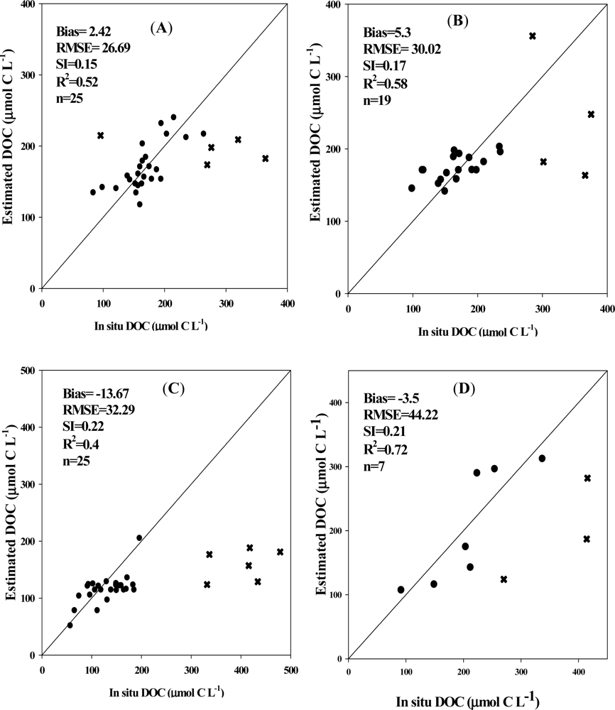
The R_rs band ratios and coefficients for both MODIS and MERIS are presented in Table 6. Surface DOC concentration maps were obtained by applying the newly developed DOC algorithms to MODIS and MERIS data (Figure 10(A,B)). To test the performance of the DOC algorithms for each sensor, the in situ DOC concentrations (μmol·C·L⁻¹) were compared with MODIS and MERIS-derived DOC (μmol·C·L⁻¹) (Figure 11(A–D)). The matchup comparisons showed estimation of DOC with Bias = −13.67, RMSE = 32.29, SI = 0.22, R² = 0.4, and N = 25 for MODIS, and Bias = −3.5, RMSE = 44.22, SI = 0.21, R² = 0.72, and N = 7 for MERIS during the spring-winter period (Table 7). The statistical parameters obtained from validation of DOC for MODIS (Bias = 2.42, RMSE = 26.59, SI = 0.15, R² = 0.52, and N = 25) and for MERIS (Bias = 5.3, RMSE = 30.02, SI = 0.17, R² = 0.58, and N = 19) during the summer period are shown in Table 7. The statistical analysis verifies acceptable performance of the DOC algorithm for MERIS in the northern Gulf of Mexico in both the summer and spring-winter periods.

The empirical algorithm for CDOM is: a_CDOM (412) = ln[(R_rs ratio − A)/B]/(−C), and the equations for seasonal DOC are: DOC = 127.027 ln[(R_rs ratio − A)/B]/(−C) + 77 for the spring-winter season, DOC = 137.22 ln [(R_rs ratio − A)/B]/(−C) + 124.20 for summer. The coefficients are presented in Table 6.

4. Discussion

4.1. CDOM, Salinity and DOC Relationship

The conservative behavior of CDOM and DOC were examined through the correlations between DOC, CDOM, and salinity. Seasonal variability in CDOM and DOC concentration is highly dependent on the MR and AR discharges [18,46,49]. Naik et al.[49] reported that on the Atchafalaya shelf, CDOM dominates the total light absorption when Atchafalaya River flow is high, while non-algal particles (NAP) play a more important role contributing to total light absorption during low-flow conditions. Chen and Gardner [46] observed high concentrations of CDOM and DOC during high-flow conditions in the Mississippi and Atchafalaya River plume regions, as well as their seasonal variability linked to water’s residence time and plant growth cycles in the watershed. We observed that in situ DOC concentration in the lower Atchafalaya River was ∼35% on average higher than DOC concentration in the lower MR during the spring-winter period and is similar (∼20%–30%) to the results reported by Wang et al.[50] for April 2001. The elevated DOC and CDOM in the lower Atchafalaya River plume is likely due to the interaction of the Atchafalaya River with the adjacent productive and extensive salt marshes, wetlands and bayous, while in comparison such interactions are less for the Mississippi River [37,46]. The strong inverse linear correlation between a_CDOM(412) and salinity observed in summer (R² = 0.77), and in the spring-winter period (R² = 0.86) suggests that terrestrial allochthonous CDOM behaved conservatively in the study area. Sampling in low salinity, high CDOM waters during summer likely masked the effects of light-induced photobleaching. The strong correlation between CDOM absorption coefficient at 412 nm and DOC concentration shows that the distribution of DOC was also highly influenced by physical mixing between two-end members, indicating conservative behavior of DOC. However, the relationship during summer suggests loss of CDOM in comparison to DOC.

4.2. CDOM and DOC Retrieval Algorithms

In assessing the performance of two empirical CDOM algorithms for SeaWiFS, it was found that the percentage differences between SeaWiFS-estimated CDOM and field CDOM associated with the D’Sa et al.[18] and the LM algorithm for CDOM retrieval were 10% and 61%, respectively. Poor performance of the LM algorithm could be due to an interference from chlorophyll-a and particulate organic carbon (POC) in the Rrs(490)/R_rs(555) ratio. In comparison, the R_rs band ratio (R_rs(510)/R_rs(555)) proposed by D’Sa et al.[18] is less affected by chlorophyll-a and POC [51–53] exhibiting high accuracy in CDOM retrievals for summer, while spring-winter was not evaluated due to lack of data. These results also suggests that the DOC algorithm based on D’Sa et al.[18] R_rs band ratio performs well in the northern Gulf of Mexico.

The matchup comparison between in situ a_CDOM(412) and MODIS-derived CDOM showed an overestimation of CDOM by MODIS (24%, the percentage difference between satellite estimated CDOM and field CDOM) which could due to interference by chlorophyll-a on the R_rs(488)/R_rs(555) band ratio used for a_CDOM(412) retrieval. However, other factors such as the time difference between satellite overpass and field measurement, pixel box size, and errors and uncertainties associated with satellite-derived R_rs used to develop the empirical algorithm can accentuate these discrepancies. Since CDOM concentration is highly variable spatially and temporally in our study area, appropriate available time difference (less than 5 h) and pixel box size (1 × 1) could improve these disparities.

The empirical algorithm developed for MODIS failed for a_CDOM(412) values larger than 1.5 (m⁻¹) in CDOM-rich coastal and estuarine waters. Strong underestimation of MODIS-derived CDOM values (for values larger than 1.5 m⁻¹) in coastal waters could be related to the sediment resuspension and errors associated with atmospheric correction algorithms in turbid waters [54]. In addition, Osburn et al.[55] hypothesized that intermolecular charge transfer may be disrupted in CDOM-rich sources that are exposed to increasing salinities. Furthermore, it is more likely that the selected pixel box size and time difference, which were limited by cloud coverage, sun glint, and lack of swath, exacerbated the inaccuracy of CDOM retrieval.

Table 8. Summary of outlier stations excluded from CDOM matchup comparison for MODIS.

Station#	1	2	3	4	5
Date	20080209	20080602	20080209	20070913	20080602
Latitude	29.573	29.352	29.539	29.350	29.316
Longitude	−92.043	−89.913	−92.080	−89.910	−89.942
In situ aCDOM(412)	2.292	2.660	1.529	1.706	2.381
MODIS-derived aCDOM(412)	0.812	0.869	0.623	0.425	0.777
Pixel box size	3 × 3	3 × 3	1 × 1	3 × 3	3 × 3
Time difference (h)	+10	−5	+7	−4	−12

presents the stations’ information along with selected pixel box size and time difference for some stations mainly located at the mouth of Barataria and Vermilion Bays that were excluded as outliers for the validation analysis.

As illustrated in Figure 11(A), the algorithm proposed for DOC retrieval with MODIS performs relatively well for summer, while MODIS-estimated DOC concentration was underestimated (11%, the percentage difference between MODIS-estimated DOC and field DOC) during the spring-winter period. Considering the locations of stations during the spring-winter period which were mainly in shallow waters, this underestimation could be attributed to the sediment resuspension associated with cold front passage during spring-winter season [56]. The sediment resuspension process, and the desorption of organic matter from resuspended particles and pore waters [57] contaminate remote sensing reflectance and affects light availability leading to the underestimation of DOC concentration. Since the spring-winter field data were sampled mostly from shallow areas, the effects of sediment resuspension could have been enhanced. Also, the optically inactive fraction of DOC that cannot be measured by satellite could have contributed to the elevated DOC concentration leading to further underestimation of DOC by MODIS.

The influence of cold fronts on DOC concentration has been examined by comparing the occurrences of cold fronts and the time of DOC measurements. It appears that cold front passage increases DOC concentration resulting in less agreement between measured and satellite-derived DOC estimates, while the DOC field measurement corresponding to the time when no cold front occurred exhibited higher agreement. For example on 18 April 2008, for the station located at Tiger Shoal off the Atchafalaya Bay, the in situ DOC sampling coincided with the passage of a cold front. The measured DOC concentration was 218.50 μmol·C·L⁻¹, while MODIS-derived DOC concentration was 125.84 μmol·C·L⁻¹ (53% underestimation). In contrast, on 16 April 2008 with no cold front, in situ DOC concentration at a station close to the former station was 170.9 μmol·C·L⁻¹, while MODIS-derived DOC concentration was 136.55 μmol·C·L⁻¹ (17% underestimation). This increase in DOC concentration during cold fronts is likely due to resuspension of sediments [58] and the associated high DOC [59] pore waters in northern Gulf of Mexico shelf sediments.

The better retrieval of a_CDOM(412) using R_rs(510)/R_rs(560) for MERIS than for MODIS (the percentage differences of 16% for MERIS and of 24% for MODIS) could be attributed to the use of the 510 nm band in constructing the CDOM algorithm which is less affected by chlorophyll-a than the 488 nm band used in the MODIS CDOM algorithm. However, the MERIS algorithm overestimated CDOM values by the percentage difference of 16%. This overestimation could be attributed to some factors including sediment resuspension over the shallow area, presence of chlorophyll-a, time gap, and pixel box size for CDOM retrievals. The location of stations excluded from the MERIS CDOM algorithm evaluation and considered as outliers (Figure 12) are detailed for five selected stations (

Table 9. Summary of outlier stations excluded from CDOM matchup comparison for MERIS.

Station#	1	2	3	4	5
Date	20090819	20080406	20080407	20070717	20050523
Latitude	28.90	29.573	29.05	29.57	29.03
Longitude	−89.47	−92.04	−90.01	−92.04	89.58
In situ aCDOM(412)	0.74	3.27	1.22	1.53	0.09
MERIS-derived aCDOM(412)	0.31	0.59	0.50	0.83	0.43
Pixel box size	3 × 3	3 × 3	1 × 1	3 × 3	1 × 1
Time difference (h)	10	24	6	14	8

). Stations located at Louisiana Bight are highly affected by MR sediment plume as a result of westward coastal current and clockwise gyre generally present in the region [60,61], whereas stations located in the Atchafalaya-Vermilion Bay region are influenced by AR sediment plume. Optical interference of suspended sediments and other photoreactive constituents in surface waters can interfere with the CDOM signal received by the sensor, and could lead to significant errors in CDOM estimates by MERIS sensor. Also, large time gaps between satellite overpasses and in situ sampling, and pixel box size used in CDOM retrievals could likely further deteriorate the performance of the CDOM algorithm in these dynamic coastal waters (Table 9).

MERIS estimates of DOC shows the percentage differences of 3% and 1.7% for summer and spring-winter respectively, and compared to the error associated with MODIS, the MERIS estimation shows greater accuracy. This could be due to the geographical location of stations used for MERIS DOC algorithm evaluation. While the stations used for evaluation of the DOC algorithm for MODIS were mostly located in shallow water, the stations used for testing the DOC algorithm for MERIS were located mostly in deeper water (Figure 12, for summer time). The stations’ location in deep water suggests that satellite derived band ratios were less affected by coastal water turbidity. Similar to MODIS, outlier points located in estuarine and coastal areas were excluded from DOC algorithm evaluation analysis. The DOC algorithm failed at these stations due to the effect of the same factors that caused MODIS DOC algorithm failure.

5. Summary and Conclusion

The relationship between CDOM and DOC, as well as an assessment of CDOM and DOC retrieval algorithms using SeaWiFS, MODIS, and MERIS were addressed in this study. Field measured CDOM and DOC obtained from different research cruises covering areas over the Louisiana shelf in 2005 and from 2007 to 2009 were employed to evaluate and develop CDOM and DOC retrieval algorithms. Conservative DOC and CDOM behavior for both summer and spring-winter periods were observed in the study area. These conservative relationships were used to develop empirical algorithms to derive DOC concentration from satellite ocean color sensors.

In comparing the D’Sa et al.[18] algorithm with the LM algorithm for CDOM estimation and further for DOC estimation, the D’Sa et al.[18] SeaWiFS algorithm performed relatively well. Similar processes were followed to develop a DOC algorithm for MODIS and MERIS sensors. For MODIS, R_rs(488)/R_rs(555) values were obtained from satellite data and correlated with a_CDOM(412), while for MERIS, R_rs(510)/R_rs(560) values were used to construct a band ratio empirical algorithm. A comparison of satellite-derived with in situ a_CDOM(412) revealed that both MODIS and MERIS tend to overestimate CDOM values < 1.5 m⁻¹, and both algorithms failed for CDOM values > 1.5 m⁻¹. Several factors may contribute to these discrepancies such as optical interference of chlorophyll-a, time difference between satellite overpass and field measurements, and the selected pixel box size. In addition, the seasonal relationship between a_CDOM(412) and DOC was combined with the a_CDOM(412)-R_rs ratio to construct DOC seasonal empirical algorithms. Then satellite-derived DOC values were correlated against in situ DOC values to test their performance. In summer, both sensors performed reasonably well, while in the spring-winter period there was a tendency for underestimation of DOC particularly for MODIS, likely due to sediment resuspension by cold front intrusions or time difference between in situ and satellite passes.

The approach followed in this study was based on available field and satellite data. As mentioned in the discussion section, some spatial and temporal limitations associated with available data introduced significant errors and uncertainties. In order to develop more robust empirical algorithms to estimate DOC concentration and gain insight about DOC dynamics, future measurements of physical and optical properties should be obtained at high temporal and spatial resolution and coincident with satellite overpasses. Since SeaWiFS and MERIS are no longer operational, and MODIS is exceeding its nominal six-year design lifetime, developing new algorithms for new sensors and their validation against the in situ data is required.

References

- Hansell, D.A.; Carlson, C.A. Biogeochemistry of total organic carbon and nitrogen in the Sargasso Sea: Control by convective overturn. Deep-Sea Res 2001, 48, 1649–1667. [Google Scholar]
- Jiao, N.; Herndl, G.J.; Hansell, D.A.; Benner, R.; Kattner, G.; Wilhelm, S.W.; Kirchman, D.L.; Weinbauer, M.G.; Luo, T.; Chen, F.; et al. Microbial production of recalcitrant dissolved organic matter: Long-term carbon storage in the global ocean. Nat. Rev. Microbial 2010, 8, 593–599. [Google Scholar]
- Ogawa, H.; Tanoue, E. Dissolved organic matter in oceanic waters. J. Oceanogr 2003, 59, 129–147. [Google Scholar]
- Gandhi, H.; Wiegner, T.N.; Ostrom, P.H.; Kaplan, L.A.; Ostrom, N.E. Isotopic (13C) analysis of dissolved organic carbon in stream water using an elemental analyzer coupled to a stable isotope mass spectrometer. Rapid Commun. Mass Spectrom 2004, 18, 903–906. [Google Scholar]
- Fichot, C.G.; Benner, R. A novel method to estimate DOC concentrations from CDOM absorption coefficients in coastal waters. Geophys. Res. Lett 2011. [Google Scholar] [CrossRef]
- Coble, P.G. Marine optical biogeochemistry: The chemistry of ocean color. Chem. Rev 2007, 107, 402–418. [Google Scholar]
- Del Castillo, C.E.; Miller, R.L. On the use of ocean color remote sensing to measure the transport of dissolved organic carbon by the Mississippi River Plume. Remote Sens. Environ 2008, 112, 836–844. [Google Scholar]
- Griffin, C.G.; Frey, K.E.; Rogan, J.; Holmes, R.M. Spatial and interannual variability of dissolved organic matter in the Kolyma River, East Siberia, observed using satellite imagery. J. Geophys. Res. 2011. [Google Scholar] [CrossRef]
- Coble, P.G.; Hu, C.; Gould, R.W., Jr.; Chang, G.; Wood, A.M. Colored dissolved organic matter in the coastal ocean. Oceanography 2004, 17, 50–59. [Google Scholar]
- D’Sa, E.J.; Miller, R.L.; Mckee, B.A. Suspended particulate matter dynamics in coastal waters from ocean color: Application to the northern Gulf of Mexico. Geophys. Res. Lett 2007. [Google Scholar] [CrossRef]
- Carder, K.L.; Chen, F.R.; Lee, Z.P.; Hawes, S.K.; Kamykowski, D. Semianalytic Moderate-Resolution Imaging Spectrometer algorithms for chlorophyll-a and absorption with bio-optical domains based on nitrate-depletion temperatures. J. Geophys. Res 1999, 104, 5403–5421. [Google Scholar]
- Hoge, F.E.; Wright, C.W.; Lyon, P.E.; Swift, R.N.; Yungel, J.K. Inherent optical properties imagery of the western North Atlantic Ocean: Horizontal spatial variability of the upper mixed layer. J. Geophys. Res 2001, 106, 129–140. [Google Scholar]
- Maritorena, S.; Siegel, D.A.; Peterson, A. Optimization of a semi-analytical ocean color model for global scale applications. Appl. Opt 2002, 41, 2705–2714. [Google Scholar]
- Siegel, D.A.; Maritorena, S.; Nelson, N.B.; Hansell, D.A.; Lorenzi-Kayser, M. Global distribution and dynamics of colored dissolved and detrital organic materials. J. Geophys. Res 2002. [Google Scholar] [CrossRef]
- Bricaud, A.; Morel, A.; Prieur, L. Absorption by dissolved organic matter in the sea (yellow substance) in the UV and visible domains. Limnol. Oceanogr 1981, 26, 43–53. [Google Scholar]
- Morel, A.; Prieur, L. Analysis of variations in ocean color. Limnol. Oceanogr 1977, 22, 709–722. [Google Scholar]
- IOCCG, Status and Plans for Satellite Ocean Color Missions: Considerations for Complementary Missions; Report Number 2; IOCCG: Dartmouth, NS, Canada, 1999; p. 5.
- D’Sa, E.J.; Miller, R.L.; Del Castillo, C. Bio-optical properties and ocean color algorithms for coastal waters influenced by the Mississippi River during a cold front. Appl. Opt 2006, 45, 7410–7428. [Google Scholar]
- Kahru, M.; Mitchell, B.G. Seasonal and nonseasonal variability of satellite-derived chlorophyll and colored dissolved organic matter concentration in the California Current. J. Geophys. Res 2001, 106, 2517–2529. [Google Scholar]
- D’Sa, E.J.; Miller, R.L. Bio-optical properties in waters influenced by the Mississippi River during low flow conditions. Remote Sens. Environ 2003, 84, 538–549. [Google Scholar]
- Johannessen, S.C.; Miller, W.L.; Cullen, J.J. Calculation of UV attenuation and colored dissolved organic matter absorption spectra from measurements of ocean color. J. Geophys. Res. 2003. [Google Scholar] [CrossRef]
- Mannino, A.; Russ, M.E.; Hooker, S.B. Algorithm development and validation for satellite-derived distributions of DOC and CDOM in the US Middle Atlantic Bight. J. Geophys. Res 2008, 113, 1–19. [Google Scholar]
- Twardowski, M.S.; Lewis, M.; Barnard, A.; Zaneveld, J.R.V. In-Water Instrumentation and Platforms for Ocean Color Remote Sensing Applications. In Remote Sensing of Coastal Aquatic Environments; Miller, R., Del Castillo, C., McKee, B., Eds.; Springer: Dordrecht, The Netherlands, 2005; pp. 69–100. [Google Scholar]
- Zhu, W.; Yu, Q.; Tian, Y.Q.; Chen, R.F.; Gardner, G.B. Estimation of chromophoric dissolved organic matter in the Mississippi and Atchafalaya river plume regions using above-surface hyperspectral remote sensing. J. Geophys. Res 2011. [Google Scholar] [CrossRef]
- Vodacek, A.; Hoge, F.E.; Swift, R.N.; Yungel, J.K.; Peltzer, E.T.; Blough, N.V. The use of in situ and airborne fluorescence measurements to determine UV absorption coefficients and DOC concentrations in surface waters. Limnol. Oceanogr 1995, 40, 411–415. [Google Scholar]
- Ferrari, G.M. The relationship between chromophoric dissolved organic matter and dissolved organic carbon in the European Atlantic coastal area and in the West Mediterranean Sea (Gulf of Lions). Mar. Chem 2000, 70, 339–357. [Google Scholar]
- Rochelle-Newall, E.J.; Fisher, T.R. Production of chromophoric dissolved organic matter fluorescence in marine and estuarine environments: An investigation into the role of phytoplankton. Mar. Chem 2002, 77, 7–21. [Google Scholar]
- Del Vecchio, R.; Blough, N.V. Spatial and seasonal distribution of chromophoric dissolved organic matter and dissolved organic carbon in the Middle Atlantic Bight. Mar. Chem 2004, 89, 169–187. [Google Scholar]
- Kowalczuk, P.; Zablocka, M.; Sagan, S.; Kulinski, K. Fluorescence measured in situ as a proxy of CDOM absorption and DOC concentration in the Baltic Sea. Oceanologia 2010, 52, 431–471. [Google Scholar]
- Bianchi, T.S.; Allison, M.A. Large-river delta-front estuaries as natural “recorders” of global environmental change. Proc. Nat. Acad. Sci. USA 2009, 106, 8085–8092. [Google Scholar]
- Van Der Leeden, F.; Troise, F.L.; Todd, D.K. The Water Encyclopedia, 2nd ed.; Lewia: Chelsea, MI, USA, 1990. [Google Scholar]
- Milliman, J.D. Flux and Fate of Fluvial Sediment and Water in Coastal Seas. In Ocean Margin Processes in Global Change; Mantoura, R.F.C., Martin, J.M., Wollast, R., Eds.; Wiley: Berlin, Germany, 1991; pp. 69–89. [Google Scholar]
- Wiseman, W.J.; Bane, J.M.; Murray, S.P.; Tubman, M.W. Small-scale temperature and salinity structure over the inner shelf west of the Mississippi River delta. Memo. Soc. Roy. Sci. Liege 1976, 6, 277–285. [Google Scholar]
- Lohrenz, S.; Fahnenstiel, G.L.; Redalje, D.G.; Lang, G.A.; Dagg, M.J.; Whitledge, T.E.; Dortch, Q. Nutrients, irradiance and mixing as factors regulating primary production in coastal waters impacted by the Mississippi River plume. Cont. Shelf Res 1999, 19, 1113–1141. [Google Scholar]
- Dinnel, S.P.; Wiseman, W.J. Fresh-water on the Louisiana and Texas shelf. Cont. Shelf Res 1986, 6, 765–784. [Google Scholar]
- Rabalais, N.N.; Wiseman, W.J.; Turner, R.E.; Sengupta, B.K.; Dortch, Q. Nutrient changes in the Mississippi River and system responses on the adjacent continental shelf. Estuar. Coast 1996, 19, 386–407. [Google Scholar]
- D’Sa, E.J. Colored dissolved organic matter in coastal waters influenced by the Atchafalaya River, USA: Effects of an algal bloom. J. Appl. Remote Sens 2008. [Google Scholar] [CrossRef]
- Conmy, R.N.; Coble, P.G.; Chen, R.F.; Gardner, G.B. Optical properties of colored dissolved organic matter in the Northern Gulf of Mexico. Mar. Chem 2004, 89, 127–144. [Google Scholar]
- Shen, Y.; Fichot, C.G.; Benner, R. Floodplain influence on dissolved organic matter composition and export from the Mississippi-Atchafalaya River system to the Gulf of Mexico. Limnol. Oceanogr 2012, 54, 1149–1160. [Google Scholar]
- D’Sa, E.J.; Dimarco, S.F. Seasonal variability and controls on chromophoric dissolved organic matter in a large river-dominated coastal margin. Limnol. Oceanogr 2009, 54, 2233–2242. [Google Scholar]
- Schaeffer, B.A.; Conmy, R.N.; Aukamp, J.; Craven, G.; Ferer, E.J. Organic and inorganic matter in Louisiana coastal waters: Vermilion, Atchafalaya, Terrebonne, Barataria, and Mississippi regions. Mar. Pollut. Bull 2011, 62, 415–422. [Google Scholar]
- D’Sa, E.J.; Steward, R.G.; Vodacek, A.; Blough, N.V.; Phinney, D. Determining optical absorption of colored dissolved organic matter in seawater with a liquid capillary waveguide. Limnol. Oceanogr 1999, 44, 1142–1148. [Google Scholar]
- D’Sa, E.J.; Steward, R.G. Liquid capillary waveguide application in absorbance spectroscopy. Limnol. Oceanogr 2001, 46, 742–745. [Google Scholar]
- Osburn, C.L.; St-Jean, G. Stable isotope analysis of dissolved organic carbon in seawater using TOC-IRMS. Limnol. Oceanogr. Methods 2007, 5, 296–308. [Google Scholar]
- Gordon, H.R.; Wang, M. Retrieval of water-leaving radiance and aerosol optical thickness over oceans with SeaWiFS: A preliminary algorithm. Appl. Opt 1994, 33, 443–452. [Google Scholar]
- Chen, R.F.; Gardner, G.B. High-resolution measurements of chromophoric dissolved organic matter in the Mississippi and Atchafalaya River plume regions. Mar. Chem 2004, 89, 103–125. [Google Scholar]
- D’Sa, E.J.; Korobkin, M. Colored dissolved organic matter in the northern Gulf of Mexico using ocean color: Seasonal trends in 2005. Proc. SPIE 2008. [Google Scholar] [CrossRef]
- Bianchi, T.S.; DiMarco, S.F.; Smith, R.W.; Schreiner, K.M. A gradient of dissolved organic carbon and lignin from Terrebonne-Timbalier Bay estuary to the Louisiana shelf (USA). Mar. Chem 2009, 117, 32–41. [Google Scholar]
- Naik, P.; D’Sa, E.J.; Grippo, M.; Condrey, R.; Fleeger, J. Absorption properties of shoal-dominated waters in the Atchafalaya Shelf, Louisiana, USA. Int. J. Remote Sens 2011, 32, 4383–4406. [Google Scholar]
- Wang, X.C.; Chen, R.F.; Gardner, G.B. Sources and transport of dissolved and particulate organic carbon in the Mississippi River estuary and adjacent coastal waters of the northern Gulf of Mexico. Mar. Chem 2004, 89, 241–256. [Google Scholar]
- O’Reilly, J.E.; Maritorena, S.; O’Brien, M.C.; Siegel, D.A.; Toole, D.; Menzies, D.; Smith, R.C.; Mueller, M.J.; Mitchell, B.G.; Kahru, M.; et al. Ocean Color Chlorophyll-a Algorithms for SeaWiFS, OC2, and OC4: Version 4. In SeaWiFS Post-Launch Calibration and Validation Analyses; Hooker, S.B., Firestone, E.R., Eds.; NASA Goddard Space Flight Center: Greenbelt, MD, USA, 2000; Volume 11, pp. 9–23. [Google Scholar]
- Stramski, D.; Reynolds, R.A.; Babin, M.; Kaczmarek, S.; Lewis, M.R.; Roettgers, R.; Sciandra, A.; Stramska, M.; Twardowski, M.S.; Franz, B.A.; et al. Relationships between the surface concentration of particulate organic carbon and optical properties in the eastern South Pacific and eastern Atlantic Oceans. Biogeosciences 2008, 5, 171–201. [Google Scholar]
- Allison, D.B.; Stramski, D.; Mitchell, B.G. Seasonal and interannual variability of particulate organic carbon within the Southern Ocean from satellite ocean color observations. J. Geophys. Res 2010. [Google Scholar] [CrossRef]
- D’Sa, E.J.; Zaitzeff, J.B.; Yentsch, C.S.; Miller, J.L.; Ives, R. Rapid Remote Assessments of Salinity and Ocean Color in Florida Bay. In The Everglades, Florida Bay, and Coral reefs of the Florida Keys: An Ecosystem Sourcebook; Porter, J.W., Porter, K.G., Eds.; CRC Press: Boca Raton, FL, USA, 2002; pp. 451–459. [Google Scholar]
- Osburn, C.L.; Retamal, L.; Vincent, W.F. Photoreactivity of chromophoric dissolved organic matter transported by the Mackenzie River to the Beaufort Sea. Mar. Chem 2009, 115, 10–20. [Google Scholar]
- Walker, N.D.; Hammack, A.B. Impacts of winter storms on circulation and sediment transport: Atchafalaya-Vermilion Bay Region, Louisiana, U.S.A. J. Coastal Res 2000, 16, 996–1010. [Google Scholar]
- Shank, G.C.; Zepp, R.G.; Whitehead, R.F.; Moran, M.A. Variations in the spectral properties of freshwater and estuarine CDOM caused by partitioning onto river and estuarine sediments. Estuar Coast. Shelf Sci 2005, 65, 289–301. [Google Scholar]
- Corbett, D.R.; Mckee, B.A.; Allison, M.A. Nature of decadal-scale sediment accumulation on the western shelf of the Mississippi River delta. Cont. Shelf Res 2006, 26, 2125–2140. [Google Scholar]
- Sutula, M.; Bianchi, T.S.; Mckee, B.A. Effect of seasonal sediment storage in the lower Mississippi River on the flux of reactive particulate phosphorus to the Gulf of Mexico. Limnol. Oceanogr 2004, 49, 2223–2235. [Google Scholar]
- Rouse, L.J.; Coleman, J.M. Circulation observations in the Louisiana Bight using LANDSAT imagery. Remote Sens. Environ 1976, 5, 635–642. [Google Scholar]
- Walker, N.D.; Wiseman, W.J.; Rouse, L.J.; Babin, A. Effects of river discharge, wind stress, and slope eddies on circulation and the satellite-observed structure of the Mississippi River plume. J. Coastal Res 2005, 21, 1228–1244. [Google Scholar]