1. Introduction
Hyperspectral imaging is a remote sensing approach that simultaneously collects both spatial and spectral data. Spectral data are collected in hundreds of narrow contiguous bands that may cover the visible, near-infrared, and short-wave infrared (0.4–2.5
μm), the mid-wave infrared (3–5
μm), and/or the long-wave infrared (8–14
μm). Although the size of a pixel on the ground varies, spatial measurements typically consist of hundreds of pixels in both spatial dimensions. Such images contain a wealth of information and have found application in a broad range of fields such as food safety [
1], agriculture [
2], mineralogy [
3], ecology [
4], planetary exploration [
5], and target detection [
6], as well as many others.
There are a number of methods for exploiting hyperspectral image data to generate useful products. One common method is spectral unmixing. This process refers to one or both of two fundamental operations. The first is the identification of spectra that are representative of the distinct materials in the scene. These spectra are referred to as endmembers and the problem of identifying them as endmember extraction. It is possible that an endmember spectrum may not be found in an image pixel, even though the associated material is present in the scene. This occurs when the material associated with that endmember does not completely fill any single pixel in the image. In that case, which is not uncommon in real data, the endmember spectrum will only be present in an image pixel in combination with other endmember spectra. Because an endmember is uniquely associated with a specific material, the terms endmember and material are used interchangeably throughout the remainder or this paper.
The second spectral unmixing operation is abundance quantification, which entails determining the proportion of each endmember in each pixel of the image. Abundance maps provide useful visualizations of hyperspectral data, showing where each endmember is located in an image and how completely each pixel is filled by that endmember. Depending on the algorithm and the application, endmembers may be determined first and subsequently utilized for abundance quantification, the endmembers and abundances may be found simultaneously, or abundances may be computed without any prior endmember information [
7].
There are a wide variety of algorithms that have been developed to unmix hyperspectral data. A recent survey article classified algorithms into one of four categories: (1) geometric; (2) statistical; (3) sparse regression based; and (4) spatial-spectral contextual [
8]. Independent component analysis (ICA) is a statistical unmixing approach that does not assume a specific distribution for the data [
9]. This approach attempts to unmix the data by finding maximally independent abundances. A variety of ICA algorithms have been applied to hyperspectral unmixing including contextual ICA [
10], joint cumulant-based ICA [
11], joint approximate diagonalization of eigenmatrices (JADE) [
12], and FastICA [
12–
15]. ICA has also been employed as a hyperspectral classification approach [
16,
17]. There are still questions regarding the utility of ICA as a hyperspectral unmixing approach. A common opinion is that while ICA can produce interesting and useful results, it is common for some materials to be incorrectly unmixed [
12,
14,
15]. Because of these lingering questions, the behavior of the FastICA algorithm [
18] is examined more closely later in this paper. FastICA was selected over other ICA algorithms because of its wide use and straightforward implementation.
Whenever spectral unmixing algorithms are assessed, two types of experiments are typically performed. In the first, synthetic images are created according to a simple generative model—usually the linear mixing model. The complexity of these images varies, but they are typically composed of 2–10 endmembers whose spectra are obtained from a real hyperspectral image or from a spectral reference library. In many cases spatial contiguity is incorporated using abundance maps consisting of simple square or circular regions. These kinds of test images are fairly common in the spectral unmixing literature [
19–
23]. Since many spectral unmixing approaches, including ICA, do not consider spatial context, synthetic images can also be produced using randomly generated abundances that adhere to some probability distribution. In these cases a generative model is used that incorporates other interesting behavior, such as topographic variation and endmembers with spectral variability [
12,
24]. In the majority of these cases the endmembers are generated in relative proportion to each other. That is, there is no single material that dominates the scene spatially and no material that is present in only a very small fraction of pixels. These images are useful because they are relatively simple to generate, and because complete ground truth data are available, including abundance maps accurate to small fractions of a pixel. Spectral unmixing results can then be compared against the ground truth data to provide quantitative assessments of algorithms.
The second type of experiment tests an algorithm by unmixing a real hyperspectral data set. The results of the unmixing are often assessed visually by recognizing landmarks in the original image and in the unmixed data [
11,
14]. In some cases ground truth data are available and can be compared with the unmixing results [
10,
20]. Unfortunately, these ground truth data often only provide information for a subset of the materials in the scene and may be incomplete for certain areas or materials in the image. They do not provide the fine abundance resolution of synthetic images and are not available for every image that might be of interest.
Both of the experimental approaches described above are useful and even essential in assessing the effectiveness and behavior of a hyperspectral algorithm. There is, however, a third approach that can be viewed as something of a middle ground between the two. This approach utilizes synthetic images that more closely approximate real data by modeling scene geometry, material properties, sensor behavior, atmospheric contributions, and so forth. Complex scene geometry is desirable because it produces images that have regions of spatial contiguity, topographic variation, and endmember spectral variability. This approach also leads to broad variations in the spatial coverage of individual materials. Because the images are synthetic, complete ground truth data are still available. Such an approach is not intended to be a replacement for the existing methods described above. Instead, it should be treated as a complementary approach, allowing for exploration of unique insights and observations.
This complementary approach could be employed to explore a variety of hyperspectral unmixing algorithms. However, throughout the remainder of this paper, it is used to assess the behavior of FastICA. This exploration is warranted to confirm existing assertions regarding FastICA and also to provide further insight into the behavior of the algorithm.
The remainder of the paper proceeds as follows. Section 2 provides a basic overview of ICA and the FastICA algorithm. It also outlines the ICA data model and compares it with the linear mixing model used to describe hyperspectral data. Section 3 explains the approach taken to generate synthetic—but realistic—hyperspectral data cubes. Examples of both image data and abundance maps are shown. Section 4 describes the experiments performed, presents the results of those experiments, and provides insight into those results. Finally, Section 5 contains a few concluding observations and remarks.
2. Independent Component Analysis
Independent component analysis (ICA) is an approach for performing blind source separation (BSS). The generalized BSS problem is modeled as
where
x(
t) = [
x1(
t)
x2(
t) ⋯
xK(
t)]
T is the
K-dimensional observed data vector,
s(
t) = [
s1(
t)
s2(
t) ⋯
sL(
t)]
T is an
L-dimensional vector of the sources of interest, and
f(·) describes the mixing process that operates on the sources to create the observed data. The observations and sources are indexed by
t, which depending on the application may represent time, spatial location, or some other quantity. In the case of hyperspectral unmixing,
t is used to index spatial location,
i.e., individual pixels. The goal of blind source separation is to estimate the original sources from the observed data with limited or no knowledge of either
f(·) or
s(
t). The estimation process is often referred to as unmixing. Blind source separation has found application in many varied areas including biomedical signal processing [
25,
26], telecommunications [
27,
28], and finance [
29,
30].
ICA is an approach that attempts to perform BSS by exploiting the statistical independence of the original sources. While this can be accomplished in a number of ways, many ICA algorithms invoke the central limit theorem [
31], observing that the distribution of mixed random variables tends toward a Gaussian distribution. Hence, sources can be separated by optimizing a cost function that reflects some measure of Gaussianity. Commonly used cost functions include kurtosis and negentropy. Other ICA approaches include minimization of mutual information [
32], and joint diagonalization of eigenmatrices [
33].
Although nonlinear ICA methods exist [
34,
35], linear mixing is most commonly assumed. In this case the mixing is represented by
where
A, is the
K × L mixing matrix and
T is the total number of observations (pixels). Stacking the observed and source data as
X = [
x(1)
x(2) ⋯
x(
T)] and
S = [
s(1)
s(2) ⋯
s(
T)], the model becomes
with the
K × T observation matrix,
X, and
L × T source matrix,
S.
The mixed data must satisfy two important conditions for ICA to be a valid unmixing approach. First, since ICA attempts to unmix the data by exploiting the independence of the sources, the sources must be independent. Second, because the methods of separation utilized by ICA algorithms attempt to maximize non-Gaussianity (based on the central limit theorem), no more than one source may be Gaussian distributed [
18].
2.1. FastICA
FastICA is an ICA algorithm that assumes the linear mixing model in
Equation (3) with the additional constraint that the number of observations must match the number of sources,
i.e.,
K =
L, making the mixing matrix
A square. The unmixing model then becomes
Y =
BX, where
Y contains the estimates of the original sources. Defining the unmixing matrix to be
a single independent component can be obtained as
or equivalently,
Since neither reordering nor scaling of the estimates affects their independence, ICA outputs are subject to scale ambiguity and order uncertainty. Because of this, any result of the form
, where
γ is a constant scalar value, is generally considered a success.
Prior to performing any source separation the observed data are whitened where
z(
t) =
Vx(
t), such that
E [
z] =
0, and
E[
zzT] =
I. Incorporating the whitened data, the unmixing model becomes
Y =
WZ =
WVX, and
B =
WV, where
W is comprised of stacked vectors as
B in
Equation (4).
As part of the whitening process the dimension of the observed data is reduced via principal component analysis (PCA). Unless specified by the user, the number of dimensions is determined automatically from the relative magnitudes of the eigenvalues of the covariance matrix of the observed data. This dimension reduction step is an attempt to estimate the number of sources and make the mixing matrix square, as required by the FastICA model.
After whitening and dimension reduction, the source separation is achieved by using a simple fixed-point algorithm to maximize a cost function. Thus, the source separation problem becomes
Typically,
G(·) in
Equation (7) is defined to be
or
The derivatives of these functions are
and
The first function is an approximation of the kurtosis of
y. Incorporating either of the other two functions gives an approximation of the negentropy of
y.
Because the whitening step effectively orthogonalizes the observed data, the unmixing matrix,
W, is constrained to be an orthogonal matrix with
WWT =
WTW =
I. This constraint is enforced at each iteration of the cost function optimization in one of two ways. If the components are extracted one at a time, deflationary orthogonalization is performed. This approach updates a single unmixing vector using the gradient optimization algorithm. That vector is then made orthogonal to all of the previously computed unmixing vectors:
The unmixing vector is then normalized as
Alternatively, if all of the components are estimated simultaneously, then symmetric orthogonalization is performed. In this case all
L unmixing vectors are updated and subsequently orthogonalized using the update formula
2.2. Application to Hyperspectral Data
One approach to modeling the radiance of a single pixel in a hyperspectral image is the linear mixing model [
36]. This model is typically formulated as
In this model
x(
t) is the observed
K × 1 pixel where
K is the number of spectral bands of the sensor. As described previously, the index
t is used to indicate the spatial location of the pixel. The
K × 1 vector
ml represents an endmember spectrum and
al(
t) is the fractional abundance of that endmember in the pixel. The total number of endmembers is
L. Instrument noise and model error are represented by
n(
t). The
K ×
L matrix
M is the endmember matrix and contains the
L individual endmembers in its columns. The
L × 1 abundance vector,
a(
t), is formed by stacking the relative abundances. The relative abundances are subject to two constraints:
and
These constraints impose the physically meaningful requirements that the fractional abundances be nonnegative and sum to one. This model is valid only when the materials in the pixel are well-partitioned from one another [
36,
37]. Even though this is not always the case in nature, this model is still widely used.
The pixels in the observed cube can be indexed in row-scanned order so that each spectral band is represented as a one-dimensional vector, rather than a two-dimensional image. Then, the terms on both sides of
Equation (17) can be stacked as
where
X and
N are
K ×
T matrices,
A is an
L ×
T matrix, and
T is the total number of pixels in the image. In this arrangement a column of
X is the spectrum of a specific pixel in the image and a row of
X contains all of the pixels from one spectral band of the data, in row-scanned order. Similarly, a column of
A describes the fractional abundances for every material in a single pixel while a row of
A contains the fractional abundance in every pixel of a single material, again in row-scanned order.
The hyperspectral mixing model in
Equation(20) is structurally similar to the linear ICA model in
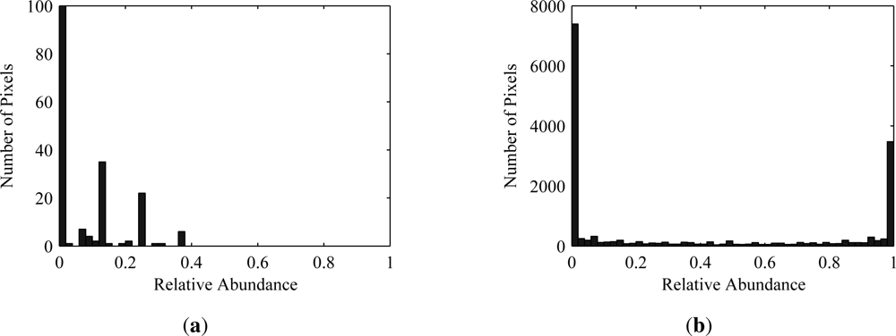
Equation(3). The endmember matrix is analogous to the mixing matrix and the abundance matrix corresponds to the source matrix. The one difference is the addition of noise in the hyperspectral model. If the signal-to-noise ratio (SNR) is sufficiently large, the noise contribution may be safely ignored, in which case the models are identical. Otherwise, the noise effects could be minimized by smoothing, dimension reduction, or some other preprocessing step. Recall that the ICA model requires the sources to be non-Gaussian, implying that the fractional abundances for each material must not have a Gaussian distribution. This requirement is satisfied as abundance values tend to accumulate near zero or one depending on their spatial coverage and have a predominantly one-sided distribution. This behavior is illustrated in
Figure 1, which shows histograms for abundance maps of two different materials generated from a three-dimensional model of a real-world scene. The other requirement imposed by ICA is that the sources be independent. For the hyperspectral data model the abundance of each material is required to be independent of every other material. This requirement is violated by the additivity constraint in the linear mixing model
Equation(19). Although this is a violation of the ICA assumptions, as the number of endmembers and/or signature variability increases, the statistical dependence of the sources decreases and ICA performance improves [
12].
3. Experimental Data Description
In order to perform the kind of complementary experiments described earlier, a means of producing realistic images and the associated ground truth data is needed. This section describes the tool employed to produce the synthetic data that were incorporated into the experiments described in subsequent sections of this paper.
The Digital Image and Remote Sensing Image Generation (DIRSIG) software is a physics-based image simulation tool developed at the Rochester Institute of Technology (RIT) [
38]. The tool allows the user to describe complex scene geometry, viewing geometry, and the spectral and thermal properties of materials in a scene. The user can also describe a variety of sensor properties including sensor type, scan behavior, focal length, detector layout, and spectral and spatial response. MODTRAN [
39] is incorporated to simulate realistic atmospheric behavior from user-provided atmospheric and weather information. Incorporating all of this information, the software employs thermal and radiometric models along with a ray tracer to compute radiance fluxes at specific points [
40]. The approach is used to generate realistic remote sensing images. Additionally, DIRSIG can also export the ground truth associated with each image.
For our experiments, two test images were generated using DIRSIG. Both images incorporate the “MegaScene” geometric scene description, which models a 0.6 square mile area of Rochester, New York. A pushbroom spectrometer model that incorporates a spectral response between 0.4
μm and 2.5
μm with 224 bands was used. The spectral response is similar to the Airborne Visible/Infrared Imaging Spectrometer (AVIRIS) [
41]. The altitude of the sensor was 2 km. With these settings in place, 1,024 × 1,024 pixel cubes and truth maps were generated with a ground sampling distance (GSD) of 0.25 m. These were then binned spatially to produce 128 × 128 pixel radiance cubes and truth maps with a GSD of 2.0 m. The binning was performed to produce data with the desired linear mixing behavior. Randomly-generated Gaussian noise was added to the data to produce cubes with a variety of signal-to-noise ratios (SNRs).
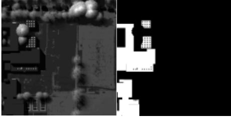
The first radiance cube generated is referred to as “Mega1” because of its location within the first tile of the MegaScene. The scene is dominated by two large buildings surrounded by a parking lot. At the top of the image is a residential road with homes on either side that are mostly obscured by trees. Three tennis courts are located at the bottom of the image. The remainder of the scene is grass. There are 43 unique materials in this scene. The second radiance cube comes from the fourth MegaScene tile and is aptly named “Mega4.” This scene contains ten large industrial tanks surrounded by some buildings and parking lots. Around the periphery of the scene are areas of trees and grass. This scene contains 21 unique materials. Examples of the synthetic data are shown in
Figure 2.
A list of the materials contained in each scene is provided in Section 5. These materials are sorted by the number of pixels in which they appear and are loosely segregated into four categories based on their spatial coverage in the image. Super-sparse materials are those with a combined coverage of less than one pixel. Materials in the sparse category typically are present in 1% or less of the image pixels and cover less than 0.5% of the image. They may or may not appear in the image as pure pixels. Dense materials appear in over half of the pixels in the image and consequently also constitute a large number of pure pixels. Materials falling between the sparse and dense categories are classified as intermediate materials. This categorization is used to analyze how materials of varying spatial distribution are affected in the spectral unmixing process. This is an example of the type of assessment that is not usually made in the two most common experimental scenarios described in Section 1.
4. Experimental Results
Three sets of experiments were performed to characterize the utility of FastICA as a hyperspectral unmixing approach. The first set of experiments examined the impact of dimension reduction on the best-case unmixing scenario. Second, the effects of orthogonalization were explored, again considering a best-case unmixing scenario. Because dimension reduction and orthogonalization are not unique to FastICA, these two experiments are of interest beyond the scope of FastICA. In the final set of experiments, unmixing was performed using FastICA. The results of these experiments are quantified by comparing estimated material abundances with corresponding abundance ground truth. The quality of endmember extraction was not considered in these experiments. Some observations are made in the following narrative on the effects of adding noise to the synthetic images, but complete characterization of the impact of noise on the unmixing process is beyond the scope of this paper.
For the remainder of this paper, whenever performance is plotted versus material,
i.e., the x-axis is “Material Number”, the materials are numbered according to the lists in the
appendix. The first (left-most) material in the plot is the most sparse and the last (right-most) is the most dense. Markers are used to denote the four categories of material spatial coverage. A circle (○) is used to identify super-sparse materials, a cross (×) for sparse materials, a diamond (⋄) for intermediate materials, and a square (□) for dense materials.
4.1. Computation of Optimal Estimates
Because complete ground truth abundance maps are available, the optimal, linear unmixing vector and corresponding abundance estimate can be calculated for each material. This was done prior to performing any experiments. These results constitute a best-case unmixing scenario,
i.e., the best result FastICA could produce, and provide a baseline against which experimental results can be compared. A common metric used in such comparisons is mean-square error (MSE),
where
â(
t) is an estimated abundance and
a(
t) is the ground truth abundance. However, MSE is not invariant to scaling, which is essential when considering ICA outputs, since they are subject to scale ambiguity. Thus, a preferred metric to MSE is the correlation coefficient, defined as
The absolute value of this metric is invariant to scaling of the arguments, as desired. Conveniently, this value also always falls in the range [0, 1]. It is used throughout the remaining experiments to quantify performance.
The unmixing formula
Equation (5) in combination with the linear mixing model for hyperspectral data
Equation (17) provides a formula for extracting individual abundances,
. Stacking this result to eliminate the spatial indexing yields
. The unmixing vector that maximizes
r(
â, a) is given by
The optimal abundance estimate is then
The optimal unmixing vectors and abundance estimates were calculated according to
Equations (23) and
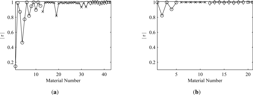
(24), respectively, for every material in both of the test cubes. In the absence of noise, as shown in
Figure 3, the maximum correlation coefficient,
r(
aˇi,
ai), is very high overall. It can be seen that the correlation coefficient tends to improve with an increase in spatial coverage. The fact that the correlation coefficient is not exactly one for every material in the scene stems from illumination, endmember, and atmospheric variability in the DIRSIG-generated cubes.
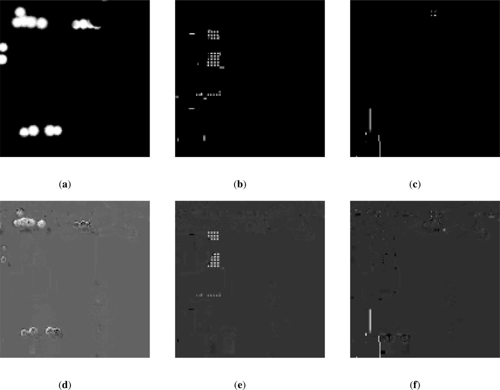
Figure 4 provides a visual comparison between ground truth and optimal estimates from Mega1 for one material from each of the four material coverage classifications. From these images it can be seen that material locations can be clearly discerned for values of |
r| ≥ 0.8. Below this threshold, the material locations are less clear and background artifacts become more obvious. Depending on the spatial coverage and congruency of a material, correlation coefficient values as low as 0.5 may be useful.
4.2. Dimension Reduction
Because it is typically used as a preprocessing step in a variety of spectral unmixing approaches, including FastICA, an experiment was performed to examine the effect of dimension reduction on the best-case unmixing scenario. To do this, the maximum correlation abundance estimates were calculated using dimension-reduced data obtained from PCA. The same maximum correlation formulas
Equations (23) and
(24) were used, replacing
X with the dimension-reduced data,
XN, given by
, where
VN is the
K ×
N whitening matrix associated with the
N most energetic principal components of
X.
The results of this experiment are shown in
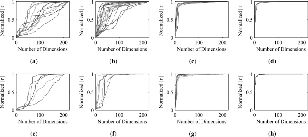
Figure 5 and
Table 1. The plots in
Figure 5 demonstrate how the correlation coefficient of the optimal estimate with the ground truth decreases as the dimensionality of the data is reduced. The correlation coefficient (y-axis) in these plots is normalized by the correlation coefficient obtained when there has been no dimension reduction. The slope of each curve illustrates the contribution of individual principal components to the correlation coefficient of the optimal estimates for a specific material. It is clear from the sharp jumps in the correlation for the dense and intermediate materials that they are well described by the first several principal components. What is also clear is that there is no similar jump for the sparse and super-sparse materials. The information associated with these materials appears to be almost uniformly scattered across all of the principal components. For this reason, a relatively large number of dimensions must be retained to achieve near-optimal estimates of these materials.
Table 1 underscores this conclusion, showing the average number of dimensions that must be kept to obtain 95% and 75% levels of the correlation coefficient obtained when no dimension reduction was performed.
One approach to determining the number of dimensions that should be retained when performing PCA is to keep as many dimensions as are needed to retain some percentage of the total variance in the image. Retaining 99.9% of the total variance in the Mega1 and Mega4 images requires only six and five dimensions, respectively. Based on the results in
Table 1, that would allow only the dense materials to be extracted at near-optimal levels.
4.3. Orthogonalization
A second experiment examined the effect of constraining the unmixing vectors to be orthogonal. Because the PCA and whitening step decorrelates the observed data, it is expected that the unmixing vectors for the whitened data should be orthogonal. In the FastICA implementation, this constraint is enforced on the unmixing vectors at the end of each iteration of the cost function optimization.
To apply the orthogonality constraint to the optimal unmixing vectors requires a minor modification to the orthogonalization formula, since the optimal vectors were not calculated using whitened data. When the data are not whitened, the formulas for deflationary orthogonalization
Equations (14) and
(15) become:
and
respectively, where
Cx is the covariance matrix of
X. The symmetric orthogonalization formula (
16) changes in a similar way:
These changes result from the fact that orthogonality of the unmixing vectors of whitened data is equivalent to
BCxBT =
I, where
B contains the unmixing vectors of the unwhitened data.
The optimal unmixing vectors calculated by
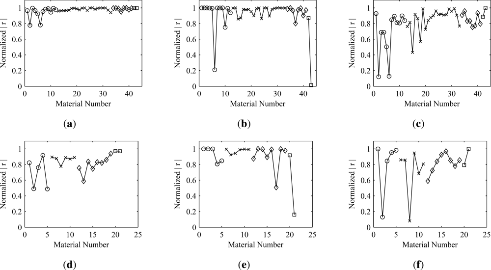
Equation (23) were forced to be orthogonal using the formulas above. Abundance estimates were then calculated from the orthogonalized vectors. The effect on the correlation coefficient of the estimates due to orthogonalization is shown in
Figure 6. Because the deflationary orthogonalization approach is sequential, the ordering of the vectors matters. The deflation was performed in both ascending and descending material order (most sparse to most dense and
vice versa). As would be expected, the results show that better estimates are obtained for those materials that are used earlier in the deflation process. Thus, to obtain better estimates of a material, it would be desirable for the cost function optimization algorithm to extract the unmixing vector corresponding to that material before any others. The results also show that deflating the estimates for more sparse materials first has less of an effect on the more dense materials than deflating in the opposite order. The symmetric approach is something of a compromise, balancing the negative effects of the orthogonalization across all of the materials.
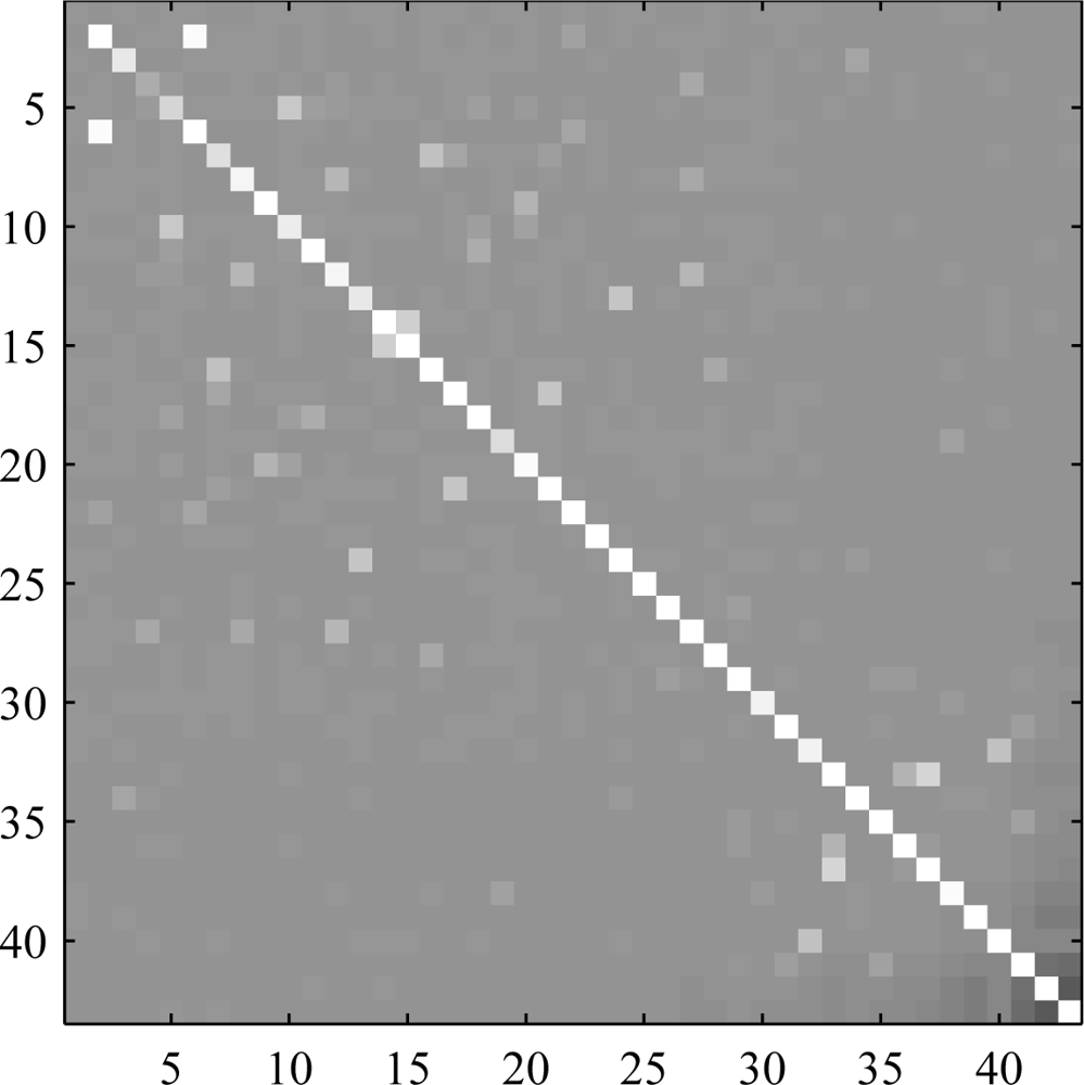
The results show that, in most cases, orthogonalization does not cause significant degradation of the estimates. This is true even in the presence of additive noise. There are a few exceptions, however, where the degradation is noticeable. Obvious examples of this are materials 2 and 6 in the Mega1 results. When symmetric orthogonalization is used, both show an appreciable decrease from the optimal correlation. When the ascending deflationary approach is used, material 2 is unaffected, but material 6 shows significant loss. Both are affected when the deflation is performed in descending material order. This behavior implies that there must be some information shared between the two materials. Thus, if material 2 is extracted first, it leads to a degradation when extracting material 6 and vice versa. Both experience degradation when the symmetric approach is used. This pattern can be explained by looking at an image representation of the matrix
BCxBT, shown in
Figure 7. If the materials were truly uncorrelated when whitened, then the image would be that of a diagonal matrix with white pixels on the diagonal and the remainder black. However, the off-diagonal bright spots in
Figure 7 indicate correlation between the optimal unmixing vectors, even when the data are whitened. In the case of this image, material 2 only shows up in one pixel and material 6 only shows up in two pixels, one of which is shared with the lone material 2 pixel. Wherever there is a drop in correlation due to orthogonalization, similar results are found,
i.e., a more sparse material shows up entirely in a subset of the pixels containing a more dense material. In these cases the additivity constraint in
Equation(19) leads to stronger correlation than for those materials that share pixels with many different materials. Therefore, while it is true that as the number of endmembers in the data increases, the statistical dependence among sources decreases and ICA performs better [
12], co-located materials with limited spatial coverage will still be poorly estimated.
