Abstract
Plot-based sampling with ground measurements or photography is typically used to establish and maintain National Forest Inventories (NFI). The re-measurement phase of the Canadian NFI is an opportunity to develop novel methods for the estimation of forest attributes such as stand height, crown closure, volume, and aboveground biomass (AGB) from satellite, rather than, airborne imagery. Based on panchromatic Very High Spatial Resolution (VHSR) images and Light Detection and Ranging (LiDAR) data acquired in the Yukon Territory, Canada, we propose an approach for boreal forest stand attribute characterization. Stand and tree objects are delineated, followed by modeling of stand height, volume, and AGB using metrics derived from the stand and tree crown objects. The calibration and validation of the models are based on co-located LiDAR-derived estimates. A k-nearest neighbor approach provided the best accuracy for stand height estimation (R2 = 0.76, RMSE = 1.95 m). Linear regression models were the most efficient for estimating stand volume (R2 = 0.94, RMSE = 9.6 m3/ha) and AGB (R2 = 0.92, RMSE = 22.2 t/ha). This study was implemented for one Canadian ecozone and demonstrated the capacity of a methodology to produce forest inventory attributes with acceptable accuracies offering potential to be applied to other boreal regions.
1. Introduction
Accurate forest information is required by a broad range of stakeholders to meet myriad information needs [1]. For instance, government institutions require forest inventory information to meet reporting and planning responsibilities [2]. Industrial forestry agencies require forest inventory data to make long term projection of volume, as well as to plan harvesting and field operations. Additionally, the roles of forests in regulating air quality, water flow, and climate regulation is well recognized [3]. Therefore accurate information on forest composition and structure is necessary.
National Forest Inventories (NFI) have been established by most countries to monitor and report on forest resources for national and international purposes [1]. In Canada the NFI is a key program of the Canadian Forest Service (CFS) dedicated to the production of information related to the structure and condition of Canada’s forests [4]. Canada’s forest area occupies approximately 400 million ha [5], representing an estimated 27.3 billion tonnes of biomass [6]. This area includes 196.3 million ha of boreal forest [6] for which limited coverage with aerial photography is available mainly due to financial and logistical constraints [7]. Forests in the northern reaches of the boreal have low productivity and are accompanied by low densities of human population, and as a result, there is a lack of an operational imperative for air photo data collection and forest inventory development.
In Canada, forest stewardship responsibilities are primarily held by provinces and territories. Each jurisdiction has an inventory program to support planning and management activities. Federally, via a sample-based NFI, there is a process to standardize measures and definitions across jurisdictions and to support collection of additional data to ensure appropriate sample coverage and to support national and international reporting obligations [2,4]. The sample based inventory is a systematic survey of 2 × 2 km photo plots on a 20 km national grid. This configuration results in a 1% sample of Canada’s land mass. A subset of ground plots is also collected in support of quality control and calibration of photo plots as required. Photo plots are akin to subsets of polygon-based forest inventory data [4]. In the southern portion of the country, where forests are more actively managed, photo plot information is typically acquired from manual interpretation of air photos. In the north, satellite data has been used to supply photo plot information, either from classified satellite imagery (a Landsat based land cover product [8]) or, more recently, from Very High Spatial Resolution (VHSR, <1-m spatial resolution) WorldView or QuickBird imagery [9]. National transects of Light Detection and Ranging (LiDAR) data have also been collected to provide field plot-like information over remote areas to enable model calibration and validation [10]. Such data sources are intended to address the lack of inventory data in northern Canada and supplant the forest attribute estimates derived from look-up tables (LUT) developed as part of the Earth Observation for Sustainable Development of forests (EOSD) project [8]. Furthermore these data sources are intended to enable greater consistency between the inventories of Canada’s northern and southern forests.
Characterization of a wide range of forest information such as stand type, crown closure, height, volume, and biomass with the use of optical satellite imagery has been proven feasible operationally for NFIs such as in northern Canada [8,11], Finland [12] and Sweden [13]. Airborne LiDAR also has a demonstrated ability to provide metrics from which accurate stand attribute estimates can be derived for large areas [14,15]. More specifically, LiDAR data has been used in sample-based protocols allowing the estimation of forest attributes outside the area covered by the LiDAR swath. Empirical and semi-empirical relationships were established between LiDAR metrics and other remote sensing-derived metrics from optical satellite imagery that enable a larger spatial coverage of the ground [16,17].
Falkowski et al. [9] proposed a series of recommendations, indicating the necessity to automate image processing techniques whenever possible, with manual interpretation of some difficult-to-capture parameters being considered when automation is not possible, inconsistent, or unreliable. Based on the framework proposed by Falkowski et al. [9], additional methodological developments have been undertaken towards automated attribute estimation requirements. For instance, Mora et al. [18] implemented a stand height estimation approach based upon an initial stand delineation procedure followed by calibration with photo-interpreted heights. This procedure used a segmentation method to create forest stands from VHSR imagery. Individual tree crown (ITC) isolation [19] was then implemented to generate individual tree objects. To enable stand level attribution, the distributions of crown objects within segments were related to stand level measurements. Using the distribution of crown objects in the approach is intended to make the routine more robust to outliers and capitalize upon image spatial information. Algorithm development with a preference towards spatial information is aimed to reduce the reliance on spectral information (that can be influenced by the sensor used, calibration approach, acquisition date, and sun-surface-sensor geometry, as examples).
In this research we have focused on further development and extension of the Mora et al. [18] protocol to be calibrated and validated using airborne LiDAR-based stand heights in place of photo-interpreted heights. The relationship between LiDAR measures and stand structure is illustrated well in Frazer et al. [20]. Further, in this study we have aimed to expand the set of stand attributes predicted to make estimates of height, volume, and biomass. To meet these goals, we have developed a logic and processing chain that enables the extrapolation of structural characteristics from plot-calibrated LiDAR measures to statistical descriptions of segment constrained individual tree crowns. First, we build models relating LiDAR-derived metrics to the field measurements; we then apply the models to predict inventory attributes for all areas covered by the LiDAR acquisition, and then we build models relating image-derived metrics (including ITC metrics) to the LiDAR predictions. Finally, we apply the models to predict inventory attributes (including height, biomass, and volume) over the entire forested area of the imagery.
In this communication we demonstrate the logic and required processing chain designed to predict boreal forest stand height, volume, and biomass. A key innovation is the use of transects of LiDAR data to calibrate and independently validate the predicted forest structural outcomes. The use of LiDAR data in this manner allows for a larger sample size than is typically possible in the northern regions of Canada, as well as the independent validation of predicted stand level structural estimates. The accuracy of the model estimates are assessed by a comparison with independent stand height, volume, and biomass estimates derived from LiDAR-based models. Although the process described is in support of Canada’s sample-based NFI VHSR framework, the challenges identified are informative for stand-based forest inventories in general, especially areas not subject to systematic and regular inventory.
2. Material and Methods
2.1. Study Area
The Boreal Cordillera has been chosen as a test ecozone [21] for this research. The Boreal Cordillera is characterized by a climate ranging from cold and sub-humid to semi-arid. The study site, near Watson Lake, has an annual mean temperature of −2.9 °C, with mean monthly daily means ranging between −24.2 °C (January) and 15.1 °C (July) [22]. Over the Boreal Cordillera the mean annual precipitation ranges from less than 300 mm in valleys shadowed by coastal mountain ranges, to more than 1,500 mm at higher elevations. The topography of the Boreal Cordillera ecozone includes mountains, extensive plateaus, and wide valleys and lowlands. Glaciation, erosion, solifluction, and eolian and volcanic ash deposition have altered the topography. Glacial drift, colluvium, and outcrops are the most common surface materials. Permafrost is widespread in the more northern areas of the ecozone. Depending on local conditions, tree species include black spruce (Picea mariana), white spruce (Picea glauca), lodgepole pine (Pinus contorta), subalpine fir (Abies lasiocarpa), balsam poplar (Populus balsamifera), quaking aspen (Populus tremuloides), and paper birch (Betula papyrifera). Wildfire, insects, and, to a lesser extent, forest harvesting are the primary forest disturbances in the Yukon Territory. Two photo plots located in southern Yukon Territory have been chosen based on the availability of spatially coincidence of panchromatic VHSR and transects of LiDAR data (Figure 1).
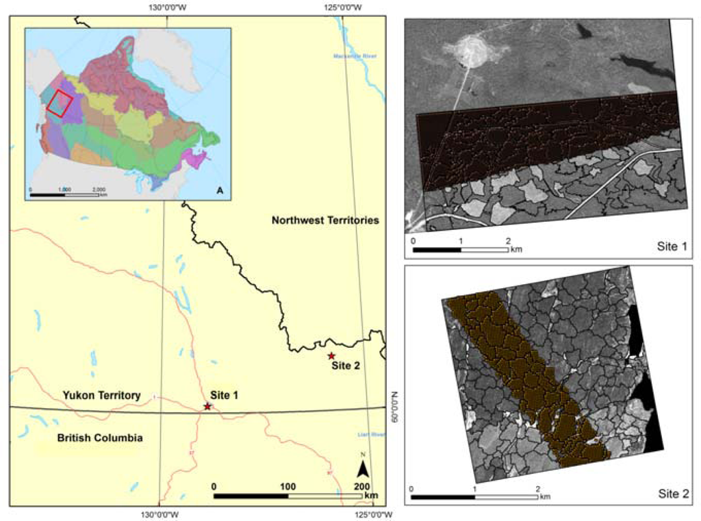
Figure 1.
Study site location. Spatial distribution of the ecozones of Canada, Sites 1 and 2: Very High Spatial Resolution (VHSR) image overlaid by stand segments and LiDAR points.
2.2. Data
Panchromatic optical satellite images were acquired for each of the two sites considered in this study. A panchromatic (0.45–0.9 μm) QuickBird-2 image (0.6 m spatial resolution) was acquired for site 1 and a panchromatic (0.4–0.9 μm) image from WorldView-1 (0.5 m spatial resolution) was acquired for site 2. Table 1 summarizes the acquisition parameters for each image. Panchromatic VHSR images have the advantage of being less costly than multi-spectral data while also providing a sufficient amount of information to enable the characterization of tree objects. This methodological aspect is critical when considering large-area forest inventories, whether they are sample-based or area-wide. Images were converted to top-of-atmosphere (TOA) spectral radiance following Krause [23,24]. The images were orthorectified using a 15 m panchromatic Landsat-7 ETM+ orthoimage [25]. Both sites had flat or gentle slopes (<5%). The average RMSE for the orthorectification was 6 m. In Figure 2, a flow diagram captures the data, methods, and sequence of the attribute estimation approach described.

Table 1.
VHSR image acquisition parameters.
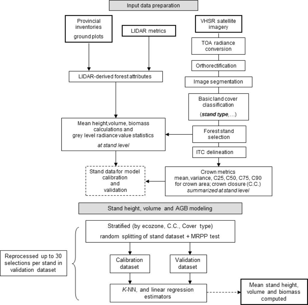
Figure 2.
Flowchart of the modeling, image processing, and attribution approach.
LiDAR data were acquired in the summer of 2010 during a national airborne mission across the boreal forests of Canada from 14 June to 20 August 2010 [10]. The CFS working with Applied Geomatics Research Group (AGRG) and the Canadian Consortium for LiDAR Environmental Applications Research (C-CLEAR) acquired 34 transects of small-footprint discrete return airborne LiDAR data. The collection of LiDAR data was designed to preferentially intersect NFI plot locations where acquisition of VSHR images was prioritized previously. The survey resulted in the collection of more than 25,000 km of LiDAR data, with a swath width that typically exceeded a specified minimum of 400 m, and a nominal point density of 3 points per m2 (for survey details see [26]). Priority areas included ecozones largely located in the boreal zone, greater than 50% forested, and less than 75% managed. A total of 34 individual survey flights were completed traversing 13 UTM zones, from Newfoundland (56°W, UTM zone 21) in the east to the Yukon (138°W, UTM zone 8) in the west. Latitudinally, the flights extended from 43° to 65°N. An Optech Airborne Laser Terrain Mapper (ALTM) 3100C discrete return sensor was used for this survey. Survey flights were made between airports with suitable runways, fuel availability, and maintenance facilities, and ranged from one to five hours in duration. The average transect length was 700 km. Table 2 provides a summary of the LiDAR survey flights and sensor characteristics. Separation of returns into ground and non-ground classes was completed using a purpose-developed method based on [27].
Table 2.
Summary of LiDAR survey flight and sensor parameters.
2.3. Calculation of LiDAR Metrics and Plot-Level Attributes
LiDAR metrics characterizing the laser point cloud (e.g., canopy cover, mean-, maximum-, and percentiles of height, among others) were calculated for 25 × 25 m grid cells (hereafter LiDAR plots; [10]) along the LiDAR transect using FUSION software [28]. Metrics were calculated using first return data above a two meter height threshold to distinguish vegetation hits from ground hits [29,30].
Field data were acquired from 201 forest inventory ground plots in Quebec, Ontario, and the Northwest Territories, and captured a representative range of boreal forest stand conditions. Ground plots had an area of 400 m2 and forest attributes were calculated using all stems greater than 9 cm in diameter. Tree height metrics and basal area were estimated for the ground plots using regionally appropriate standard inventory and mensuration equations. Using field-measured height and diameter at breast height (DBH), gross stem volume was estimated for individual trees using Equation (1) ([31]; p. 582]. Plot volumes were calculated as the sum of the individual tree volumes using a paraboloid model.
where V is the stem volume in m3, Db is the DBH in cm, and H is the tree height in m. Finally, biomass tree components were estimated using DBH- and height-based all-species equations from [32,33]. Plot biomass was calculated as the sum of the individual tree biomasses obtained via the summation of the tree component biomasses. Readers with additional interest in the relationship between LiDAR point clouds and the spatial summarization metrics developed in relation to stand structure are referred to Frazer et al. [20]. It is the LiDAR derived metrics that provide independent variables in predictive models of forest attributes developed.
Based on the statistical relationships between the aforementioned LiDAR metrics and ground plot attribute estimates, plot-level estimates of dominant height, gross stem volume, and total aboveground biomass (AGB) were then generated for the area covered by the LiDAR data using multiple linear regression models [10]. Predictors were selected for their low inter-correlations and biological relevance [34]. Akaike’s Information Criterion [35] was employed to support selection of the most parsimonious models [36].The final models for dominant height (DH) (R2 = 0.84, RMSE = 1.63 m, RMSE-% = 9), gross stem volume (VG) (R2 = 0.8, RMSE = 68.5 m3/ha, RMSE-% = 25) and total AGB (AGBT) (R2 = 0.76, RMSE = 33.7 t/ha, RMSE-% = 24) are given in Equations (2–4) respectively:
where Lhp95 is the 95th percentile of the first return heights, CC2m is the percentage of first returns above 2 m, Lhmean is mean first return height, LhCV is the coefficient of variation of first return heights, and CC2m is the percentage of first returns above 2 m [10].
2.4. Calculation of Stand-Level Metrics
Based on the VHSR images, delineation of homogeneous vegetation patterns, forest stand identification and tree crown delineation steps were implemented following the approach described in [18]. We used commercial image segmentation software (Definiens Cognition Network Technology®, München, Germany; [37,38]) to delineate segments that can be further related to homogeneous forest conditions [39] and associated with LiDAR metrics. Once segmented, each unit is attributed to a land cover class as defined per NFI and EOSD project standards [40]. Over the VHSR image extents the potential classes include: treed, herb, shrub, bryoid, wetland, exposed land, rock, snow-ice (not present), and water. The classification was verified to ensure the appropriateness of the class assignments. Next, a tree crown delineation procedure was implemented using the Individual Tree Crown (ITC) suite [20] for all the treed segments. The threshold values that determine whether a pixel belongs to a tree crown or the surrounding shadow or understory were iteratively adjusted for each image according to the vegetation distribution and structure, sun-surface-sensor geometry, and solar conditions present.
The next step comprised the calculation of a series of stand-level statistics based on the grey level values of the panchromatic images, including median, mean, standard deviation, and range in the treed segments. A second series of stand-level statistics was calculated based on the ITC-based metrics, and include crown closure, mean crown size (i.e., crown area), and the 25th, 50th, 75th, and 90th percentiles of the crown size distribution. Hereafter percentiles are noted as CX with X the value of the percentile (e.g., the 25th percentile of crown size is noted as C25). Prior to the computation of the stand metrics–crown closure excepted–crown objects with abnormal sizes were discarded from the dataset using the C5 and C95 as upper and lower thresholds respectively. These objects represented outliers (e.g., image artifacts or crowns that are beyond local size expectations), often related to clusters of trees that could not be separated for objects above the C95 threshold. Additional outlier removal was performed on stands with crown closures lower or greater than 3 standard deviations from the mean crown closure value (computed over all stands).
An inner stand buffer of 17.7 m (half of the diagonal length of a 25-m sided square) was applied to select the appropriate LiDAR plots that fell within each stand (to avoid selection of LiDAR plots that contain returns belonging to neighboring stands). Only stands with at least 10% of their area overlapped by LiDAR data and containing a minimum of fifteen 25-by-25 m LiDAR plots were considered for model calibration and validation. A weighted average of the dominant LiDAR plot height based on the number of LiDAR hits was calculated from the LiDAR plots following the procedure from [41] to estimate stand height. Stand level volume and total AGB estimates (Equations (2) and (3)) were calculated by averaging values from the LiDAR plots within each stand.
2.5. Height, Volume, and Biomass Modeling
Stand height modeling was performed with k-NN and linear regression models (Figure 2). In the modeling protocol, we identified stand level median grey level value from the VHSR data and the C90 of crown size distribution as the most suitable input variables. The protocol was based on multiple random selections that split the original dataset into calibration (60% of the stands) and validation datasets (40% of the stands). These iterative random draws were stratified according to the stand crown closure, which is known to influence the calculated stand metrics [42,43]. Modeling methods were implemented using the R software [44]. The package stats (version 2.13.2) was used for the linear regression modeling, and the package yalmpute (version 1.0–15) was used for the k-NN method [45]. The number of k neighbors to use was estimated based on the computation of one thousand random stand selections used as calibration and validation datasets followed by stand height modeling. The test was repeated for values of k ranging from 1 to 30. The value of k providing the best stand height estimations was selected for the subsequent tests. Varying distance computation methods were tested: Euclidean, Mahalanobis, two Most Similar Neighbor methods (noted MSN and MSN2), and an independent component analysis based method [45]. The final stand height corresponded to the average of the height estimates obtained from the k-NN modeling through the required iterations. Stand volume and AGB model establishment followed an identical framework as the one used for the stand height modeling with the addition of a stepwise linear regression method introduced as a first step to identify the best input metrics amongst the tested predictors.
3. Results
3.1. Stand Identification and Stand Metrics
A total of 309 segments or stands were delineated over the two images, of which 249 were classified as forest, including 88 that met the requirements for subsequent use in the calibration and validation of the models. The segmentation procedure allowed the generation of forest stands greater than 2 ha in size (the NFI standard for minimum stand area [46]) and reasonable within-stand LiDAR-derived attribute standard deviations of 16% for height (μ = 7.5 m, σ = 1.2 m), 25% for volume (μ = 60 m3/ha, σ = 15 m3/ha), and 28.5% for AGB (μ = 112 T/ha, σ = 32 T/ha). The mean stand area was 9.6 ha. Two outlier stands were excluded based on differing median grey level values caused by the presence of logging roads and low forest cover density over a portion of the stands (values of 2.6 and 2.7). As a result, the calibration and validation datasets had 52 and 34 stands, respectively. The range of crown closure values in the final dataset ranged from 34% to 49%. Table 3 summarizes stand metrics obtained from the grey level values and the delineated crowns. All forest stands identified were classified as coniferous, although some small patches of deciduous trees were identified visually. Over this particular study area the establishment of stand type specific models was not required.
Table 3.
Statistics on image grey level values and tree crowns for segment level metrics used as inputs to the models.
3.2. Stand Height Modeling
Height models considered the median grey level value in the segment (median_S) and the C90 of the stand crown size distribution as input parameters. The mean variance inflation factor (VIF) values computed across the iterations equaled 1.95 (σ = 0.1) for the linear regression method (Table 4). A R2 value of 0.71 and a RMSE value of 2.13 m (RMSE-% = 12.8) were obtained. The distribution of the residuals was normal (p = 0.8). No significant difference was found between the estimated and LiDAR measured heights for both methods (p > 0.8) and homoscedasticity was verified (p = 0.17).
Table 4.
Stand height linear regression model accuracy.
We determined that the best number of neighbors was 6 for the k-NN modeling. The best results were obtained with the Euclidean and the Mahalanobis methods with R2 values of 0.75 and 0.76, respectively and RMSE values of 1.95 for both methods (RMSE-% = 11.6) (Table 5). Figure 3(a) shows the scatter plot of the LiDAR heights and those estimated by the k-NN modeling established with the Mahalanobis distance. Figure 3(b) shows the distribution of the residuals for the best model (k-NN with Mahalanobis distance) according to the LiDAR stand heights.
Table 5.
Stand height k-NN model accuracies.
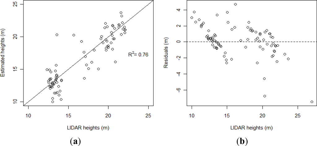
Figure 3.
(a) Scatter plot of the best estimated stand heights versus LiDAR heights (b) Residuals of the best model versus stand LiDAR height.
3.3. Stand Volume and AGB Modeling
The stepwise procedure used to select the best stand metrics to establish models identified the C25 of the crown size distribution and crown closure as the best stand metrics (with VIF values = 1) for the volume model among the suite of metrics considered. The stand height, crown closure, mean crown area, and C25, C50, C75, C90 of the crown size distribution were selected as the best predictors for the AGB model. However, for the AGB model, all the metrics had VIF values greater than 10, the crown closure excepted (VIF = 1.2). The necessity to establish statistically robust and biologically-driven models [34] led to the consideration of models based on stand height and crown closure for volume and biomass models. Stand height and crown closure are commonly used as predictors for stand volume [47] and biomass [11,48] and can also be derived through image processing and modeling. The linear regression and k-NN modeling methods were subsequently implemented using this two-metric combination (stand height and crown closure).
The stand volume model based on the linear regression method provided a R2 value of 0.94 with a VIF value of 1.08 (Table 6). Figure 4 presents the scatter plots of the best estimated volume values and the residuals of the linear regression model versus LiDAR volume values. Normality of the residuals was verified for the linear regression model (p = 0.83), homoscedasticity was verified (p = 0.73), and no significant difference was found between LiDAR-derived and estimated volumes (p = 0.97).
Table 6.
Stand volume and biomass linear regression model accuracy.
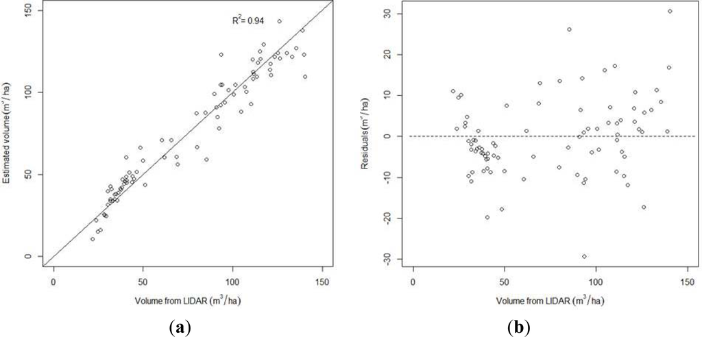
Figure 4.
(a) Scatter plot of the best estimated volume values versus LiDAR volume values (b) Residuals of the best model versus stand LiDAR volume values.
AGB models had similar trends as stand volume models, with a R2 value of 0.92 with low VIF value (1.08). Figure 5 presents the scatter plots of the best estimated AGB values and the residuals of the linear regression model versus LiDAR-derived AGB values. For the linear regression method, normality of the residuals was verified (p = 0.83), homoscedasticity was verified (p = 0.68), and no significant difference was found between estimated and LiDAR-derived values (p = 0.97).
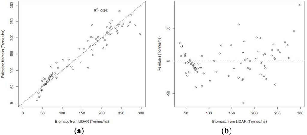
Figure 5.
(a) Scatter plot of the best estimated biomass values versus LiDAR biomass values (b) Residuals of the best model versus stand LiDAR biomass values.
For the k-NN modeling, the same distance computation methods were tested for the stand volume and AGB modeling as those employed for the stand height modeling. K-NN models provided similar results as those obtained with linear regression method (Table 7). For both models, the lowest RMSE values were provided by the MSN and MSN2 distance computation methods with an R2 of 0.93 for the volume models and an R2 of 0.91 for the biomass models.
Table 7.
Stand volume and biomass k-NN model accuracies.
4. Discussion
In this study k-NN methods provided better results compared to the linear regression method for stand height estimation. Furthermore the influence of the distance calculation method on the results (R2 and RMSE) was not found to be statistically significant (t-test) (Table 5). However the k-NN method with the Mahalanobis distance provided the best results (R2 = 0.76 and RMSE = 1.95 m (RMSE-% = 11.6). The performance of our best model compares favorably with the results of other studies modeling stand height with VHSR and discrete return LiDAR data. Chen et al. [17] built regression models based on spectral, texture, and shadow fraction metrics derived from multispectral QuickBird and LiDAR data in Quebec, Canada. Their best model provided a R2 of 0.72 and a RMSE of 3.3 m (RMSE-% = 21). Peuhkurinen et al. [49] estimated mean stand height using stand-level spectral metrics derived from IKONOS imagery and k-most similar neighbors (K-MSN) approach, with an RMSE of 3.1 m. Wulder and Seemann [16] estimated mean stand height using segmented Landsat-5 TM and LiDAR data with a R2 of 0.67 and a RMSE of 3.3 m. Using regression, Maselli et al. [50] extended a sample of LiDAR-derived mean stand height estimates over 798 ha area using Landsat ETM+ data, resulting in an RMSE of 3.01 m.
The best volume and AGB models compare well with models previously established in similar forest environments. Chen et al. [17] obtained a R2 of 0.72 and a RMSE of 52.59 m3/ha for the volume model and a R2 of 0.72 and a RMSE of 39.5 tonnes/ha for the biomass. Hall et al. [11] proposed a method (BioSTRUCT: Biomass estimation from stand STRUCTure) to estimate a series of stand metrics for the EOSD initiative that represent the only consistent source of forest information in the north of Canada. Applied in Alberta, Canada, the regression models were built based on the same stand metrics used in our study (height, crown closure) but were derived from Landsat ETM+ and field plot data. In this study from Hall et al. [11], an adjusted R2 of 0.71 was obtained with a RMSE of 74.7 m3/ha for volume. For AGB an adjusted R2 of 0.70 and a RMSE of 33.7 tonnes/ha were obtained. A similar approach for AGB estimation considering equivalent input metrics derived from LiDAR data has also been used by Næsset and Gobakken [51] with canopy density (a measure of the proportion of laser echoes >2 m to the total number of echoes) replacing crown closure (R2 = 0.88 and RMSE = 21%).
Errors in stand height, volume, and biomass estimates may be attributed to a number of factors. First, satisfactory model performances were reported by [10] for the field-plot inventory attribute models (dominant height, gross stem volume and AGB) with R2 values ranging from 0.76 to 0.84 and RMSE-% values ranging from 9 to 25. However, a greater number of field plots could have improved representation of the diverse forest conditions found throughout the Canadian boreal forests that were surveyed, and may have lead to improved model accuracies. Stand-level attribute models would have subsequently benefited from more accurate plot-level estimates. Second, as a result of the limited number of VHSR images collected in the study area, it was not possible to obtain images with equivalent acquisition conditions (off-nadir view angle notably). This causes variability in the results of the crown delineation procedure and in the stand-level grey-level statistics for the pool of images used to build a given model. Third, the relationship between crown diameter, DBH, and the estimated stand attributes [52,53] can be subject to alteration by a series of factors such as age and wind conditions. As a consequence, increased variability of the stand-level crown metrics used as model input can be expected. Due to a long distance to markets and relatively small trees, the study area has only limited harvesting activity with a stand structure that is largely the result of historic wildfire conditions. In addition, future applications should aim at considering satellite image acquisition angular conditions, rather than solely regional conditions (i.e., ecozone-specific in this study case), for constraining algorithm development.
To mitigate these sources of error, we recommend the purchase of images with equivalent or as near-equivalent acquisition conditions, as possible. In addition, we recommend the use of a sufficient number of images per ecozone (≥3 from our experience) that intersect with the LiDAR transects to obtain sufficient stands for building statistically robust models, while ensuring representativeness of forest conditions. A similar reasoning should be applied to the location of the field plots used to calibrate the LiDAR data. Moreover, if stand type information is already available for the area of interest, one should check stand age, potential disturbances, and ensure a sufficient number of deciduous stands will be depicted by the VHSR and LiDAR data. This requirement may be difficult to fulfill for every ecozone in northern regions where the presence of deciduous trees may be rare. In addition, it is important to provide stand height, volume, and biomass values derived from an iterative process that aggregates multiple estimates to mitigate bias that could result from a single or a low number of random stand selections when calibration and validation datasets are generated.
Currently, when aiming to purchase VHSR imagery for national monitoring purposes we stipulate that the cloud cover tolerance over the actual 2 km × 2 km NFI photo plots is zero. Vendors are supplied with our national photo plot locations to interrogate the imagery for cloud-free status. We also limit the off nadir view angles to a maximum of 15 degrees. The view angle limitations are not specified based upon the particular look direction (that is, side to side versus fore/aft pointing). Combining these basic constraints serves to limit the number of scenes that can be obtained in a given year. While further specifying the desirable criteria for imagery suitable for inclusion in our processing chain, we are also mindful that tightening of the criteria will result in increased difficulty in obtaining imagery and our capacity to implement a sample based protocol. At present the yield of VHSR imagery on an annual basis is limited, and found to be below the number of images required to maintain our inventory reporting cycle.
In building towards this research, the capacity of VHSR imagery to capture forest inventory information was undertaken [54]. We found that VHSR could be automatically segmented to produce spatial units akin to forest stand polygons and that an interpreter could label the stands in a manner similar to traditional photography [18]. Following a review of the potential for automation of forest inventory practices using VHSR [9], experimentation demonstrated the utility of within-stand crown objects for characterizing forest structural attributes [18]. From this base research, a number of the components required of a framework for using VHSR imagery to provide otherwise unavailable information in support of the NFI were developed and aspects tested in this research. The current focus was upon stand height, volume, and biomass—a subset of attributes required for forest inventory and reporting.
Readers may note that the results achieved in this study using VHSR are similar to results achieved in other studies using Landsat (that is, RMSE ∼ 3 m, e.g., [16,50]). The question that then arises is therefore to what benefit is the cost and effort requirements of the VHSR approach presented herein, when the results are similar to results obtained using Landsat data? Moreover, a Landsat implementation to generate stand height would likely be simpler, more cost effective, and cover a larger area (with an image footprint of 185 km × 185 km rather than the approximate 10 km × 10 km of a typical VHSR image). Firstly, inventories require more than height (or volume and biomass for that matter), so the ability to interpret additional detailed information from VHSR imagery is an asset. While stand height, volume, and biomass do not constitute the entirety of an inventory, each is amongst the more important of the suite of attributes that are generated. Stand height information is important for management purposes and is indicative of site conditions, while volume is key to industrial forest management and biomass is a critical attribute for informing on forest function and carbon-related considerations. If an intimation of future recommendations can be suggested, it is that VHSR imagery (and related automated processing approaches) may remain focused on locations where jurisdiction-driven inventory programs persist, with the photo analogous data provided by the VHSR offering compatibility and similarity in the types of information generated. For areas that are not subject to regular management or monitoring activities, it is possible that the more limited suite of attributes that can be estimated from Landsat data will prove sufficient for many monitoring and reporting needs. Thus, a stratification of activity may be possible based upon the monitoring requirements associated with a given area. The ability to characterize large areas with Landsat data for a number of important forest inventory attributes may prove sufficient, although additional applications research and contextual consideration is required.
This work also encourages the further implementation of the protocol to other areas of Canada’s boreal forest. The research is aimed to determine if such an implementation for the north of Canada may offer an improved monitoring and reporting capacity. We propose that the approach demonstrated be considered to support other large-area jurisdictional or national level activities where similar characteristics are present. Further, large-area, wall-to-wall characterization with a high level of attribute detail are difficult to obtain, with sampling offering a practical, robust, and reliable alternative. Future global forest inventory programs may benefit from consideration of the framework and methods presented herein. We also note that depending on location and attributes required, wall-to-wall mapping with medium spatial resolution data (i.e., Landsat), calibrated and validated with samples of LiDAR [10], may provide analogous opportunities for systematic and repeatable monitoring and reporting activities.
5. Conclusion
The objective of this study was to apply, the complete chain of processing steps to produce stand level predictions of height, volume, and biomass from Light Detection and Ranging (LiDAR) and Very High Spatial Resolution (VHSR) imagery appropriate for a sample based forest inventory. The attribute predictions are preceded by the delineation of forest stands, the identification of the stand type, and crown closure. The use of LiDAR data allows for a large sample appropriate for model calibration and independent validation of attribute predictions. In this research we demonstrated the utility of VHSR imagery, calibrated with samples of LiDAR from a transect-based survey, to produce stand height (RMSE = 1.95 m), volume (RMSE = 9.9 m3/ha), and biomass (RMSE = 22.8 t/ha) estimates with an accuracy suitable for operational activities. This approach using statistics, sampling, LiDAR, and satellite imagery demonstrates the state-of-the-art for reporting on remote areas not subject to photo-based forest inventory programs. We also note the difference in information content between different spatial resolutions of imagery, with opportunities existing for medium spatial resolution imagery (i.e., Landsat) if a full forest inventory attribute suite is not required.
Acknowledgments
Christopher Bater (previously of UBC and now with the Government of Alberta) is thanked for his analysis efforts and insights in the development of the forest structural attributes from the LiDAR metrics. Chris Hopkinson (previously of Nova Scotia Community College and now with the University of Lethbridge) is thanked for his transect project partnership and his leadership of the national Canadian Consortium for LiDAR Environmental Applications Research (C-CLEAR) which was critical in obtaining the research data used in this study. Trevor Milne of Gaiamatics is thanked for assisting with the development of customized code for processing the long LiDAR transect files.
- Conflict of InterestThe authors declare no conflict of interest.
References
- Tomppo, E.O.; Gschwantner, T.; Lawrence, M.; McRoberts, R.E. National Forest Inventories: Pathways for Common Reporting; Springer: New York, NY, USA, 2010. [Google Scholar]
- Wulder, M.A.; Kurz, W.; Gillis, M. National level forest monitoring and modelling in Canada. Progr. Plan. 2004, 61, 365–381. [Google Scholar]
- Millennium Ecosystem Assessment. Living Beyond Our Means: Natural Assets and Human Well-Being (Statement from the Board); United Nations Environment Programme (UNEP), 2005. Available online: http://www.unep.org/maweb/en/BoardStatement.aspx (accessed on 13 March 2013).
- Gillis, M.D.; Omule, A.Y.; Brierly, T. Monitoring Canada’s forests: The National Forest Inventory. Forest Chron. 2005, 81, 214–221. [Google Scholar]
- Natural Resources Canada, Canada’s National Forest Inventory: Photo Plot Guidelines; Version 1.1; Natural Resources Canada: Victoria, BC, Canada, 2004.
- Power, K.; Gillis, M.D. Canada’s Forest Inventory 2001; Natural Resources Canada Canadian Forest Service Pacific Forestry Centre: Victoria, BC, Canada, 2006. [Google Scholar]
- Wulder, M.A.; Campbell, C.; White, J.C.; Flannigan, M.; Campbell, I.D. National circumstances in the international circumboreal community. Forest Chron. 2007, 83, 539–556. [Google Scholar]
- Wulder, M.A.; White, J.C.; Cranny, M.; Hall, R.J.; Luther, J.E.; Beaudoin, A.; Goodenough, D.G.; Dechka, J.A. Monitoring Canada’s forests. Part 1: Completion of the EOSD land cover project. Can. J. Remote Sens. 2008, 34, 549–562. [Google Scholar]
- Falkowski, M.J.; Wulder, M.A.; White, J.C.; Gillis, M.D. Supporting large-area, sample-based forest inventories with very high spatial resolution satellite imagery. Progr. Phys. Geogr. 2009, 33, 403–423. [Google Scholar]
- Wulder, M.A.; White, J.C.; Bater, C.W.; Coops, N.C.; Hopkinson, C.; Chen, G. Lidar plots—A new large-area data collection option: Context, concepts, and case study. Can. J. Remote Sens. 2012, 38, 600–618. [Google Scholar]
- Hall, R.J.; Skakun, R.S.; Arsenault, E.J.; Case, B.S. Modeling forest stand structure attributes using Landsat ETM+ data: Application to mapping of aboveground biomass and stand volume. For. Ecol. Manage 2006, 225, 378–390. [Google Scholar]
- Tomppo, E.O.; Tuomainen, T. Finland. In National Forest Inventories: Pathways for Common Reporting; Tomppo, E.O., Gschwantner, T., Lawrence, M., McRoberts, R.E., Eds.; Springer: New York, NY, USA, 2010; pp. 185–206. [Google Scholar]
- Axelsson, A.L.; Ståhl, G.; Söderberg, U.; Petersson, H.; Fridman, J.; Lundström, A. Sweden. In National Forest Inventories: Pathways for Common Reporting; Tomppo, E.O., Gschwantner, T., Lawrence, M., McRoberts, R.E., Eds.; Springer: New York, NY, USA, 2010; pp. 541–553. [Google Scholar]
- Næsset, E.; Gobakken, T.; Holmgren, J.; Hyyppä, H.; Hyyppä, J.; Maltamo, M.; Nilsson, M.; Olsson, H.; Persson, Å.; Söderman, U. Laser scanning of forest resources: The Nordic experience. Scand. J. For. Res. 2004, 19, 482–499. [Google Scholar]
- Wulder, M.A.; Bater, C.W.; Coops, N.C.; Hilker, T.; White, J.C. The role of LiDAR in sustainable forest management. Forest Chron. 2008, 84, 807–826. [Google Scholar]
- Wulder, M.A.; Seemann, D. Forest inventory height update through the integration of lidar data with segmented Landsat imagery. Can. J. Remote Sens. 2003, 29, 536–543. [Google Scholar]
- Chen, G.; Hay, G.J.; St-Onge, B.A. GEOBIA framework to estimate forest parameters from lidar transects, Quickbird imagery and machine learning: A case study in Quebec, Canada. Int. J. Appl. Earth Obs. Geoinf. 2012, 15, 28–37. [Google Scholar]
- Mora, B.; Wulder, M.A.; White, J.C. Segment-constrained regression tree estimation of forest stand height from very high spatial resolution panchromatic imagery over a boreal environment. Remote Sens. Environ. 2010, 114, 2474–2484. [Google Scholar]
- Gougeon, F.A. A crown-following approach to the automatic delineation of individual tree crowns in high spatial resolution aerial images. Can. J. Remote Sens. 1995, 21, 274–284. [Google Scholar]
- Frazer, G.; Wulder, M.A.; Niemann, K.O. Simulation and quantification of the fine-scale spatial pattern and heterogeneity of forest canopy structure: A lacunarity-based method designed for analysis of continuous canopy heights. For. Ecol. Manage 2005, 214, 65–90. [Google Scholar]
- Ecological Stratification Working Group (ESWG), A National Ecological Framework for Canada; Government of Canada: Ottawa/Hull, QC, Canada, 1995.
- Canadian Climate Normals or Averages 1971–2000. Available online: www.climate.weatheroffice.gc.ca/climate_normals (accessed on 13 March 2013).
- Krause, K. Radiance Conversion of QuickBird Data—Technical Note; DigitalGlobe Inc.: Longmont, CO, USA, 2003. [Google Scholar]
- Krause, K.S. WorldView-1 pre and Post-Launch Radiometric Calibration and Early On-Orbit Characterization; DigitalGlobe Inc.: Longmont, CO, USA, 2008. [Google Scholar]
- Wulder, M.A.; Loubier, E.; Richardson, D. Landsat-7 ETM+ orthoimage coverage of Canada. Can. J. Remote Sens. 2002, 28, 667–671. [Google Scholar]
- Hopkinson, C.; Wulder, M.A.; Coops, N.C.; Milne, T.; Fox, A.; Bater, C.W. Airborne Lidar Sampling of the Canadian Boreal Forest: Planning, Execution, and Initial Processing. Proceedings of SilviLaser, Hobart, TS, Australia, 16–19 October 2011; pp. 393–401.
- Axelsson, P. DEM generation from laser scanner data using adaptive TIN models. ISPRS Int. Arch. Photogramm. Remote Sens. Spat. Inf. Sci. 2000, 33, 110–117. [Google Scholar]
- McGaughey, R.J. FUSION/LDV: Software for Lidar Data Analysis and Visualization (No. Version 2.90); Version 2; US Department of Agriculture: Seattle, WA, USA, 2010. [Google Scholar]
- Nilsson, M. Estimation of tree heights and stand volume using an airborne LiDAR system. Remote Sens. Environ. 1996, 56, 1–7. [Google Scholar]
- Næsset, E. Practical large-scale forest stand inventory using a small-footprint airborne scanning laser. Scand. J. For. Res. 2004, 19, 164–179. [Google Scholar]
- Marshall, P.M.; Lemay, V. Forest Inventory. In Forestry Handbook for British Columbia; The Forestry Undergraduate Society, University of British Columbia: Vancouver, BC, Canada, 2005; pp. 577–604. [Google Scholar]
- Lambert, M.-C.; Chhun-Huor, U.; Raulier, F. Canadian national tree aboveground biomass equations. Can. J. For. Res. 2005, 35, 1996–2018. [Google Scholar]
- Ung, C.-H.; Bernier, P.; Guo, X.-J. Canada national biomass equations: New parameter estimates that include British Columbia data. Can. J. For. Res. 2008, 38, 1123–1132. [Google Scholar]
- Li, Y.; Andersen, H.-E.; McGaughey, R.J. A comparison of statistical methods for estimating forest biomass from light detection and ranging data. Western J. Appl. For. 2008, 23, 223–231. [Google Scholar]
- Akaike, H. Information Theory and an Extension of the Maximum Likelihood Principle. In Second International Symposium on Information Theory; Academiai Kiado: Budapest, Hungary, 1973; pp. 267–281. [Google Scholar]
- Posada, D.; Buckley, T.R. Model selection and model averaging in phylogenetics: Advantages of akaike information criterion and bayesian approaches over likelihood ratio tests. Syst. Biol. 2004, 53, 793–808. [Google Scholar]
- Baatz, M.; Schäpe, A. Multiresolution Segmentation—An Optimization Approach for High Quality Multiscale Image Segmentation. Proceedings of Angewandte Geographische Informationsverarbeitung XII, Beiträge zum AGIT-Symposium Salzburgz, Karlsruhe, Germany, 5–7 July 2000; pp. 12–23.
- Definiens, eCognition 4 User Guide; Definiens: Munich, Germany, 2004.
- Wulder, M.A.; White, J.C.; Hay, G.J.; Castilla, G. Towards automated segmentation of forest inventory polygons on high spatial resolution satellite imagery. Forest Chron. 2008, 84, 221–230. [Google Scholar]
- Wulder, M.A.; Nelson, T. EOSD Land Cover Classification Legend Report; Version 2; Canadian Forest Service Natural Resources Canada: Victoria, BC, Canada, 2003. [Google Scholar]
- Næsset, E. Determination of mean tree height of forest stands using airborne laser scanner data. ISPRS J. Photogramm. 1997, 52, 49–56. [Google Scholar]
- Parker, G.G.; Lowman, M.; Nadkarni, N. Structure and Microclimate of Forest Canopies. In Forest Canopies: A Review of Research on a Biological Frontier; Lowman, M.D., Nadkarni, N.M., Eds.; Academic Press: San Diego, CA, USA, 1995; pp. 73–106. [Google Scholar]
- Asner, G.P.; Scurlock, J.M.O.; Hicke, J.A. Global synthesis of leaf area index observations: Implications for ecological and remote sensing studies. Glob. Ecol. Biogeogr. 2003, 12, 191–205. [Google Scholar]
- R Development Core Team. R: A Language and Environment for Statistical Computing, Reference Index Version 2.2.1; R Foundations for Statistical Computing: Vienna, Austria, 2005; Available online: http://www.r-project.org/ (accessed on 13 March 2013).
- Crookston, N.L.; Finley, A.O. YaImpute: An R Package for kNN Imputation. J. Stat. Softw. 2008, 23, 1–16. [Google Scholar]
- Natural Resources Canada, The State of Canada’s Forests: Annual Report 2012; Natural Resources Canada: Ottawa, ON, Canada, 2012.
- Paine, D.P.; Kiser, J.D. Aerial Photography and Image Interpretation; John Wiley and Sons: Hoboken, NJ, USA, 2003. [Google Scholar]
- Popescu, S.C.; Wynne, R.H.; Nelson, R.F. Measuring individual tree crown diameter with LiDAR and assessing its influence on estimating forest volume and biomass. Can. J. Remote Sens. 2003, 29, 564–577. [Google Scholar]
- Peuhkurnen, J.; Maltamo, M.; Vesa, L.; Packalén, P. Estimation of forest stand characteristics using spectral histograms derived from an IKONOS satellite image. Photogramm. Eng. Remote Sensing 2008, 74, 1335–1341. [Google Scholar]
- Maselli, F.; Chiesi, M.; Montaghi, A.; Pranzini, E. Use of ETM+ images to extend stem volume estimates obtained from LiDAR data. ISPRS J. Photogramm. 2011, 66, 662–671. [Google Scholar]
- Næsset, E.; Gobakken, T. Estimation of above- and below-ground biomass across regions of the boreal forest zone using airborne laser. Remote Sens. Environ. 2008, 112, 3079–3090. [Google Scholar]
- Zhang, L. Cross-validation of non-linear growth functions for modelling tree height-diameter relationships. Ann. Bot. 1997, 79, 251–257. [Google Scholar]
- Bechtold, W.A. Largest-crown-width prediction models for 53 species in the western United States. Western J. Appl. For. 2004, 19, 245–251. [Google Scholar]
- Wulder, M.A.; White, J.C.; Hay, G.J.; Castilla, G. Towards automated segmentation of forest inventory polygons on high spatial resolution satellite imagery. Forest Chron. 2008, 84, 221–230. [Google Scholar]
© 2013 by the authors; licensee MDPI, Basel, Switzerland This article is an open access article distributed under the terms and conditions of the Creative Commons Attribution license ( http://creativecommons.org/licenses/by/3.0/).