Article

Optical and Thermal Remote Sensing of Turfgrass Quality, Water Stress, and Water Use under Different Soil and Irrigation Treatments

by
Saleh Taghvaeian
1,*,
José L. Chávez
1,
Mary J. Hattendorf
2 and
Mark A. Crookston
2
1
Department of Civil and Environmental Engineering, Colorado State University, Fort Collins, CO 80523, USA
2
Northern Colorado Water Conservancy District, Berthoud, CO 80513, USA
*
Author to whom correspondence should be addressed.
Remote Sens. 2013, 5(5), 2327-2347; https://doi.org/10.3390/rs5052327
Submission received: 11 March 2013 / Revised: 9 May 2013 / Accepted: 9 May 2013 / Published: 14 May 2013

Abstract

:
Optical and thermal remote sensing data were acquired at ground level over several turfgrass species under different soil and irrigation treatments in northern Colorado, USA. Three vegetation indices (VIs), estimated based on surface spectral reflectance, were sensitive to the effect of reduced water application on turfgrass quality. The temperature-based Grass Water Stress Index (GWSI) was also estimated by developing non-transpiring and non-water-stressed baselines. The VIs and the GWSI were all consistent in (i) having a non-linear relationship with the water application depth; and, (ii) revealing that the sensitivity of studied species to water availability increased in order from warm season mix to Poa pratensis L. and then Festuca spp.. Implemented soil preparation treatments had no significant effect on turfgrass quality and water stress. The differences between GWSI-based estimates of water use and the results of a complex surface energy balance model (METRIC) were not statistically significant, suggesting that the empirical GWSI method could provide similar results if the baselines are accurately developed under the local conditions of the study area.

Graphical Abstract

1. Introduction

In recent decades, a fast population growth along with high rates of urbanization has exacerbated the pressure on water managers to meet urban water requirements. Such a pressure is substantially greater for municipalities in arid/semi-arid regions (e.g., western USA), where water resources are scarce and in high demand. Besides the effects of population growth, some of the predicted changes in climate, such as higher summer temperatures, prolonged droughts, and less snow pack in the mountains will influence both supply and demand in such a way that meeting urban water requirements will be even more challenging in the future. Boland [1] argued that since freshwater is over-allocated in many parts of the world and it is not feasible to make new water resources available, the best solution to mitigate possible consequences of climate change relies in demand management rather than in supply development. Even in the regions where developing new water supplies is still feasible, long-term planning and significant monetary investments are required for building additional infrastructure to store water. Demand management, however, is less time and money consuming and less dependent on the uncertain effects of climate change [1].
In arid/semi-arid areas, landscape watering could be significantly larger than other uses of fresh water by urban residents (e.g., hygiene, drinking, cooking). Kjelgren et al. [2] reported that landscape irrigation accounts for about one third of the annual municipal water use of Denver, CO, USA. It should be noted that such an estimate includes winter months, when landscape water use is negligible. Hence, the same ratio would be significantly larger if winter months are excluded. For instance, Cooley and Gleick [3] reported that landscape water use during summer months can reach up to 90% of the total municipal water use in southwestern USA. This is mainly due to the fact that in these areas summer rainfall is not sufficient to provide landscape vegetation with the amount of water needed to achieve the level of aesthetic appearance that is desired by home and business owners and therefore irrigation is intensified. Hence, improving landscape irrigation management is necessary to foster sustainable management of urban water resources in the western USA [4]. Turfgrass has been the focus of irrigation studies during the past few decades, as it is one of the most dominant components of urban landscapes [5]. Carrow [6] categorized the methods for identifying the appropriate timing of turfgrass irrigation into three groups: (i) based on soil moisture depletion; (ii) based on climatic data and reference evapotranspiration; and, (iii) using canopy characteristics such as temperature and visible signs of stress. The third approach seems to have received more attention in comparison to the former methods. For example, visible rating of turfgrass quality has been extensively utilized by researchers and practitioners. However, visual assessment is a subjective process that highly depends on the assessor’s definition of aesthetically appealing. Bell et al. [7] found that visual rates of turfgrass quality were inconsistent among three human evaluators. In addition, several researchers have used a visual rating scale of one to nine [810], while others have employed a range of one to ten [11,12] or one to six [13]. Developing objective and easy-to-use methods of irrigation scheduling can lead to water conservation and can prevent the loss of nutrients from turfgrass systems [2].
Optical and thermal remote sensing techniques can be used by turf managers in a consistent and non-destructive fashion to evaluate the quality and irrigation needs of turfgrass systems, before stress signs intensify enough to become perceptible to human eyes [7,9,1416]. Previous studies have showed that spectral reflectance of turfgrass in different visible and near-infrared portions of the electromagnetic (EM) spectrum is sensitive to several factors including, but not limited to: fertilizer and herbicide application rates [9,12]; carbon concentrating mechanism (C3 vs. C4 grasses) [9]; irrigation amount and uniformity [14]; and, management practices such as mowing height [11]. In addition to optical remote sensing, several thermal remote sensing methods have been used in quantifying turfgrass water stress and water consumption. In particular, the Crop Water Stress Index (CWSI) has proved to be an effective method compared to other irrigation scheduling methods [17]. As a dimensionless ratio, CWSI determines where the measured temperature differential between plant canopy and air (dT) falls on a range of possible values for any given climatic condition. The lower limit of this range corresponds to non-water-stressed conditions, when the rate of vegetation water use or evapotranspiration (ET) is only limited by atmospheric demand (i.e., water vapor deficit). As transpiring water is the main process responsible for cooling plants, the upper limit of dT is reached when there is no water available to be used by the plant (non-transpiring conditions). There are two different approaches to estimate CWSI: (i) physically-based [18]; and (ii) empirical [19]. In the former approach, lower and upper limits of dT are modeled based on the partitioning of the available energy at the vegetative surface into sensible and latent heat fluxes. Hence, it requires numerous environmental variables before it can be applied. The latter approach, however, requires only a few easy-to-obtain variables that are used to define linear regression relationships (baselines) between the upper (non-transpiring) and lower (non-water-stressed) limits of dT and the atmospheric water vapor pressure deficit (VPD).
Since the CWSI method is implemented in this study to evaluate the presence and severity of stress in turfgrass communities (and not agricultural crops), the term Grass Water Stress Index (GWSI) will be used instead hereafter. Both the physically-based and the empirical approaches of GWSI have been previously implemented to study water stress in turfgrass systems under varying hydro-climatological conditions. Several researchers have reported that the empirical approach fails to provide an accurate estimation of dT baselines for different turfgrass species such as bermudagrass (Cynodon dactylon L.) [20], Kentucky bluegrass (Poa pratensis L.) [21], creeping bentgrass (Agrostis stolonifera L) [10,21], and tall fescue (Festuca arundinacea L.) [22,23]. All of these studies have reported that the poor performance was mainly due to the fact that upper and lower dT limits were not only a function of VPD, but also the incoming irradiance. For example, Jalali-Farahani et al. [20] observed about three units of increase in the intercept of the non-water-stressed baseline when net radiation increased from 200 to 600 W·m−2. Payero et al. [23] also reported 5.7 units of increase in intercept and 1.2 units of decrease in slope of the non-water-stressed baseline as solar radiation increased from zero to 1,000 W·m−2. A similar study of several crops showed that the lower dT limit under shaded conditions was always smaller than the same value under sunlit conditions, with a 3.8 °C difference on average at VPD of 3.6 kPa [24]. Such a dependence on incoming irradiance was not observed when the method was developed by Idso et al. [19], since input data were all collected close to solar noon and only if “the crops did not experience significant shading due to clouds.” Therefore, it is not surprising that the empirical approach does not perform well under conditions different that those it was developed under. The effect of incoming irradiance would be negligible if the clear-sky guidelines are followed in estimating dT limits based on the empirical approach.
The present study was conducted in northern Colorado in the semi-arid western USA in order to find out if optical and thermal remote sensing techniques were efficient in monitoring the quality, water stress, and water use of several turfgrass species under different soil and irrigation treatments. More specific research objectives were as follows:
  • To investigate the sensitivity of several vegetation indices to soil preparation and water application treatments in order to explore the possibility of replacing them with the traditional visual rating, performed by human assessors;
  • To estimate the GWSI based on the empirical approach and to identify the effects of experimental treatments on this stress indicator;
  • To compare the performance of several turfgrass species under limited levels of water availability; and,
  • To estimate turfgrass water use based on the GWSI approach, as well as a complex surface energy balance model.
To the best of our knowledge, the GWSI method has been mainly used to identify the timing of irrigations. Hence, using GWSI to estimate turfgrass water use will assist irrigation managers to identify both the timing and the amount of irrigation events, using the same index.

2. Methods and Materials
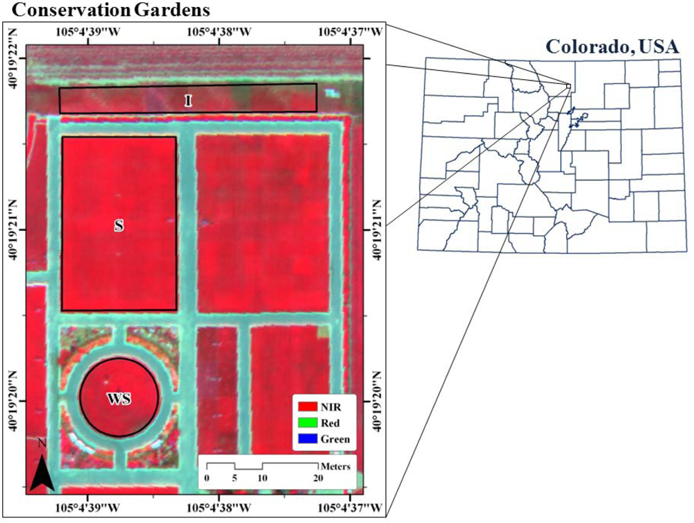
2.1. Study Area

This experiment was conducted during the summer of 2011 (20 July–27 September) at the Conservation Gardens (Lat: 40°19.3′, Long: −105°4.6′, Alt: 1,548 m) in Berthoud, northern Colorado, USA. The Conservation Gardens are a research and demonstration site developed and managed by the Irrigation Management Department at the Northern Colorado Water Conservancy District (Northern Water hereafter). This site was established to provide landscape owners and professionals with information on water-conserving practices and it includes several turfgrass species under different soil and water treatments. Figure 1 demonstrates a false-color multispectral airborne image of the study site. The experiment focused on two major treatments. The first treatment was a variable irrigation depth treatment (treatment I hereafter), where sprinklers were installed at only one side of five rectangular plots, resulting in a water application rate that decreased with distance from sprinklers. For each turfgrass plot, remote sensing readings were taken at four distances from the line-source sprinklers, namely 1.0, 2.1, 3.3, and 4.5 m. According to irrigation application records (audit), the average irrigation rate was about 13 mm·h−1 at the closest distance, which resulted in a total application depth of 190 mm during the study period. As a result, the Water Application Adequacy (WAA), defined as the ratio of applied water (gross depth of irrigation and precipitation) divided by the total grass reference ET (ETo) during the same period was 74%. At the farthest distance, irrigation rate was only 5 mm·h−1, resulting in a total irrigation depth of 73 mm and a WAA of 38%. The five plots of turfgrass mixes or blends included in this treatment were:
(i)
Warm-season mix, WSM: a mixture of 70% blue grama (Bouteloua gracilis L.) and 30% buffalograss (Bouteloua dactyloides L.);
(ii)
Aggressive Kentucky bluegrass (Poa pratensis L.), AKB: a blend of cultivars ‘Rampart’ (50%), ‘Touchdown’ (25%), and ‘Orfeo’ (25%);
(iii)
Texas hybrid bluegrass (Poa arachnifera L.), THB: a blend of cultivars ‘Reveille’ (50%) and ‘SPF 30’ (50%);
(iv)
Fine fescue, FF: a mixture of 25% ‘Covar sheep fescue’ (Festuca ovina L.), 25% ‘Intrigue Chewings fescue’ (Festuca rubra subp. Commutata), 25% ‘Cindy Lou Creeping Red fescue (Festuca rubra subp. Rubra), and 25% ‘Durar Hard fescue (Festuca trachyphylla (Hack.) Krajina); and,
(v)
Tall fescue (Festuca arundinacea L.), TF: 100% ‘Major League’ cultivar.
The second treatment was a soil preparation treatment (treatment S hereafter), where Kentucky bluegrass (Poa pratensis L.) was sodded under two different tillage depths (0.15 and 0.38 m) and three levels of organic amendments (0.0, 247, and 494 m3·ha−1 of plant waste compost), each with two replicates. Required weather variables were obtained from an on-site automated standard weather station that was owned, operated and maintained by Northern Water. This weather station was installed at a well-maintained Kentucky bluegrass plot. Weather variables were measured every 3 s and averaged and recorded on an hourly basis, using a data-logger (Model CR1000, Campbell Scientific, Logan, UT, USA). Table 1 provides information on key weather data during the study period, obtained from the Northern Water website ( http://www.northernwater.org) in November 2011. Table 2 presents the list of experimental plots, their abbreviations, and their corresponding gross irrigation depth applied during the study period. Except for treatment factors, all other influencing factors (e.g., fertilizer applications, mowing, etc.) were similar among experimental plots, attempting to provide the most favorable condition for turfgrass growth.

2.2. Remote Sensing Data

Turfgrass spectral reflectance was obtained using a hand-held, multi-spectral radiometer (model MSR5, CROPSCAN Inc., Rochester, MN, USA) that was equipped with two sets of upward- and downward-looking detectors in five wavebands centered at blue (485 nm), green (560 nm), red (660 nm), near infrared (NIR, 830 nm), and short-wave infrared (SWIR, 1650 nm) parts of the EM spectrum. These wavebands are selected in a fashion to be compatible with sensors on-board the Landsat Thematic Mapper 5 satellite. Each sensor has a 28° field of view (FOV), resulting in a circular target area with a diameter that is half of the height of radiometer above the target. Downward looking sensors detect reflected radiance in the mentioned five bands, while the upward looking sensors measure the incoming radiation through a flashed, opal glass, cosine diffuser. Obtained information was then sent to a multichannel data-logger controller, where surface reflectance in each band was computed as the ratio of downward to upward radiations considering temperature and sun angle cosine correction [25]. To be able to measure turfgrass temperature, a pre-calibrated infrared thermometer or IRT (model IRt/c.2, Exergen Corp., Watertown, MA, USA) with a 35° FOV was attached to the MSR5 radiometer. Measurements of IRT were synchronized with radiometer measurements and all of the data were sent to the data-logger controller for analyses and recording. Turfgrass temperature and reflectance were measured using the combined IRT/radiometer on seven dates during the 70 days of study period. The entire data collection over all plots took 37 minutes on average and it was always within two hours of the solar noon, under cloud-free conditions. To take the readings, the sensors were held at a nadir view angle and about 1 m above the surface. In order to provide more replication in space, four readings were taken over different spots of each experimental plot. This resulted in four readings for each level of treatment I and eight readings for each level of treatment S, since the latter treatment had two replicates. The average of four/eight readings was used in the analysis.

2.3. Vegetation Indices

The optical remote sensing data collected by the multi-spectral radiometer were further analyzed to assess the effects of turfgrass species and implemented treatments on spectral signatures. Three Vegetation Indices (VIs) were calculated and used in the analyses to explore the potentials and limitations of utilizing VIs as an alternative to the traditional visual rating approach that is currently implemented by turfgrass professionals. These VIs were the Normalized Difference Vegetation Index (NDVI) [26], the Soil Adjusted Vegetation Index (SAVI) [27], and the Visible Atmospherically Resistant Index (VARI) [28]:
NDVI = ( ρ 830 ρ 660 ) / ( ρ 830 + ρ 660 )
SAVI = ( 1.0 + L ) ( ρ 830 ρ 660 ) / ( ρ 830 + ρ 660 + L )
VARI = ( ρ 560 ρ 660 ) / ( ρ 560 + ρ 660 ρ 485 )
where ρ485, ρ560, ρ660, and ρ830 are surface reflectance in the blue, green, red, and NIR parts of the EM spectrum. The parameter L is a coefficient that changes with canopy density, but a value of 0.5 is found to be a good representative over a wide range of densities [27].
The NDVI was selected in this study because it is one of the most commonly used VIs and previous studies have shown that it is highly correlated with turfgrass visual assessment rates [7,11,12,29]. Compared to other VIs, NDVI is more sensitive to sparse vegetation, which makes it ideal for evaluating turfgrass growth and quality. A major caveat, however, is that this VI becomes less sensitive at denser canopies. Since turfgrass is usually kept at a very short height (unlike many agricultural crops), the saturation of NDVI would not impose a major challenge for turfgrass management. The selection of SAVI was based on the fact that it is efficient in minimizing the effect of soil surface wetness. In other words, when underlying soil is viewed by the remote sensing sensor, wet and dry soil surfaces would not cause a significant variation in the value of SAVI [27]. Finally, VARI was utilized in this study because it is based on the reflectance in only the visible part of the EM spectrum, and thus it would provide a quantification of turfgrass quality that is the closest to human’s eye perception. This VI is developed in a fashion to be less sensitive to the effect of atmosphere on radiation attenuation [28]. As a result, it can be successfully applied to air- and space-borne imagery without the need to account for the atmospheric optical thickness. The visible radiation is reflected at the topmost layer of the canopy. Hence, VARI can be interpreted as a color indicator. The NDVI and SAVI, on the other hand, take into account the reflected radiation in NIR waveband, which interacts with more layers of leaves. Thus, NDVI and SAVI can be regarded as plant growth and health indicators.

2.4. Grass Water Stress Index

The GWSI can be estimated using the following equation [18,19]:
GWSI = ( dT m dT LL ) / ( dT UL dT LL )
where dT is the temperature difference between the turfgrass canopy and the air, measured at a height above the canopy. Subscripts m, LL, and UL represent measured, lower limit, and upper limit of dT, respectively. All of the variables in Equation (4) have the units of temperature, resulting in a dimensionless ratio that theoretically varies between zero and unity. Besides dTm that is obtained by measuring turfgrass and air temperatures, the lower and upper limits of dT need to be known in order to calculate GWSI. As mentioned before, the empirical approach of Idso et al. [19] was implemented in this study to model dT limits using the following equations:
dT LL = m ( VPD ) + b
dT UL = m ( VPG ) + b
where “m” is the slope and “b” is the intercept of the linear relationship, VPD is the water vapor pressure deficit of the air, and VPG is the vapor pressure gradient (both in kPa), estimated as the change in saturated vapor pressure when the air temperature is increased by an amount equal to the coefficient “b”. Due to its empirical nature, the coefficients of Idso’s method are plant- and site-specific. To develop Equation (5), estimated VPD data were plotted against dTm values that were collected over healthy turfgrass after significant irrigation or precipitation events, when non-water-stressed conditions prevailed. Under these conditions, dTm can be assumed equal to dTLL. In addition, dTUL was calculated using Equation (6). To verify their accuracy, resulted dTUL values were compared with dTm values that were measured over a non-transpiring patch of turfgrass. Surface non-transpiring conditions were achieved by spraying a small patch of grass with glyphosate, which inhibited grass photosynthetic activities and therefore the transpiration process.

2.5. Turfgrass Water Use

Turfgrass water consumption was estimated using two independent methods: a GWSI-based method and a surface energy balance model known as METRIC [30].

2.5.1. GWSI-Based Water Use

According to Jackson et al. [18], GWSI is inversely related to the actual plant transpiration (Ta) in such a way that a maximum GWSI (unity) translates into no water use and a minimum GWSI (zero) corresponds to Ta rates as high as the potential (disease- and stress-free) transpiration rates (Tp):
T a = ( 1 GWSI ) T p
Equation (7) is based on the assumption that GWSI ranges between zero and unity. Obtaining GWSI values that meet this criterion requires an accurate estimation of the upper and lower dT limits. If dTm values fall beyond the range that is defined by baselines, GWSI estimates will be either negative or greater than one, resulting in Ta values that are larger than the potential rate or negative, respectively. Thus, appropriate limits were applied to GWSI values to ensure that Equation (7) did not result in unreasonable Ta estimates. The Tp values were calculated through multiplying the basal crop coefficients of cool-season grass reported in [31] and the ETo estimates obtained following the ASCE-EWRI guidelines for standardized Penman-Monteith method described in [32]. The required weather variables were collected at the on-site weather station.

2.5.2. METRIC-Based Water Use

METRIC (Mapping ET at high Resolution with Internalized Calibration) is a satellite-based remotely sensed surface energy balance model that relies on the simplified form of the energy balance equation at land surfaces [30]:
R n = G + H + LE
where Rn is net radiation, G is soil heat flux, H is sensible heat flux, and LE is the latent heat flux, all in units of energy (e.g., W·m−2). The first three components (Rn, G, and H) are estimated by integrating remotely sensed and in situ weather data, while LE is calculated as the residual of Equation (8). In this study, Rn and G were estimated following the equations and steps provided in [30]. The only difference was in estimating surface albedo, which was based on the equation provided in [33]. METRIC takes advantage of a novel approach in modeling H, which was pioneered by Bastiaanssen et al. [34]. Based on this approach, spatially distributed values of H are estimated by interpolating between two extreme conditions and by iteratively correcting the aerodynamic surface resistance and friction velocity for the effects of atmospheric stability, using the Monin-Obukhov similarity theory [30]. The extreme conditions are defined by identifying the so-called hot and cold pixels. The cold pixel is selected over a well-irrigated field, where all of the available energy (Rn − G) is used for changing the state of water from liquid to gas. The hot pixel is selected over a dry bare soil, where LE approaches zero due to the lack of available water.
Application of METRIC in the present research had two major differences with regular applications of METRIC to satellite imagery. The first difference was in the selection of the cold pixel and the performance of the internalized calibration. In METRIC, the cold pixel is selected in an agricultural area as one of the coolest pixels with a large biomass (leaf area index greater than 4). In the internalized calibration of METRIC, the ET of such a cool and tall agricultural crop is assumed to be 5% larger than the alfalfa reference ET (ETr). Therefore, ETr values estimated at a standard weather station (located within or close to the area of interest) are multiplied by a 1.05 factor and the results are regarded equal to the total LE flux at the selected cold pixel. The value of H is then estimated for this pixel using Equation (8). In this study, however, the cold pixel was selected over a recently-irrigated, stress-free turfgrass at full cover that had the coolest temperature. The fact that the cold pixel was selected over a short plant such as turfgrass rather than a tall crop such as alfalfa may introduce some error, mainly due to the fact that under similar non-water-stressed conditions, turfgrass has a lower rate of water use compared to alfalfa or other tall crops [30]. This difference was compensated for in the present study by modifying the internalized calibration process of METRIC in two ways: (i) instead of ETr, the grass reference ET (ETo) was assigned to the latent heat flux of the selected cold pixel; and, (ii) the multiplication by 1.05 coefficient was avoided. In other words, it was assumed that the available energy over the selected turfgrass cold pixel is equal to the ETo rate estimated at the on-site weather station. For the hot pixel, readings were taken over a dry, bare soil surface that was located close to the experimental treatments and had been cultivated during previous years, so it was not compacted. This is in compliance with the guidelines of METRIC about hot pixel selection [30].
The second difference between current and regular applications of METRIC was the difference in sensor platforms. While air- and space-borne images are acquired at the same instance over a large area, ground-based data used in this study were collected over the experimental plots at slightly different times. Since the entire data collection period took only 37 minutes on average (with hot and cold pixel readings taken at approximately half time), the error introduced by data collection asynchronism is not expected to be large. It should be noted that despite the temporal concurrence in data collection in regular applications of METRIC to imagery, the LE flux estimated at a standard weather station based on high-frequency data collected during a 60-minute period is used to calculate the instantaneous H flux over the selected cold pixel. In other words, it is assumed that the 60-minute LE flux is similar to the LE flux at the instance of overpass, which may have happened at any time during the 60-minute period.
The results of models that are based on remotely sensed data (e.g., GWSI and METRIC) represent surface conditions at the moment of data collection. Therefore, they should be extrapolated to longer periods (e.g., daily) for most practical applications. METRIC suggests the use of ETrF extrapolation method, which is based on the assumption that the instantaneous ratio of ETa to ETr (ETrF) remains constant throughout the day [30]. Once this ratio is estimated, it can be multiplied by daily ETr to provide an estimate of daily water use. In this study, however, the ratio of ETa to ETo (EToF) was used for extrapolating the METRIC results, not only because it is more compatible with the proposed modified internalized calibration, but also because previous studies have shown that the EToF method performs better than ETrF under advective conditions of arid/semi-arid regions [3537]. A similar approach (ETcF) was used to extrapolate GWSI-based water use estimates. This approach is explained in details by Taghvaeian et al. [38]. In order to obtain the cumulative water use of turfgrass species during the 70 days of study, water use estimates of each method (GWSI and METRIC) were interpolated for the days in between the data collection dates, following the procedure outlined in [30].

3. Results and Discussion

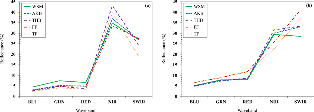
3.1. Spectral Characteristics of Turfgrass
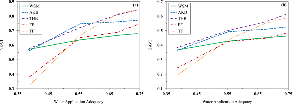
The optical remote sensing data revealed interesting patterns in the spectral characteristics of turfgrass species. Figure 2, for example, compares the spectral signature of turfgrass species in treatment I, measured at two different distances from the sprinklers and averaged for all measurement dates. The spectral signature at the closest distance was similar to that presented in [5]. At this location, 38% of the incident radiation in NIR waveband was reflected on average, an indication of large number of hydrated cell walls and air cavities in the mesophyll tissue of turf blades. However, the average reflectance in the same waveband decreased to 28% at the farthest distance from sprinklers. Another noticeable change was the overall increase in reflectance at the three visible bands as irrigation rate decreased. In other words, all turfgrass species that received higher rates of irrigation were darker in color. Similar changes in surface reflectance at the visible and NIR wavebands caused by irrigation treatments were observed in Las Vegas, Nevada for tall fescue [14], annual ryegrass [12], and bermudagrass [29]. Previous studies have shown that the SWIR waveband is the most appropriate one in the optical part of the EM spectrum for monitoring water status of plant canopies [39], since at this waveband, the incoming radiation is absorbed by the moisture content of plant parts. Our results showed that SWIR reflectance of turfgrass increased with the decrease in WAA. This means that turfgrass canopies that received less amount of irrigation were also at higher levels of wilting (less turgid). The average SWIR reflectance at closest distance was 25%, which increased to 35% at the farthest distance from sprinklers. The spectral signatures of the FF and TF species at the farthest distance resembled that of a bare soil surface, due to the effects of the reduced irrigation rate.
Evaluating the effects of irrigation treatments on turfgrass quality was also performed by comparing the VIs. Figure 3 illustrates the variation in NDVI, SAVI, and VARI with the change in WAA. Based on the observed pattern, the following conclusions can be made:
(i)
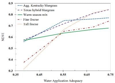
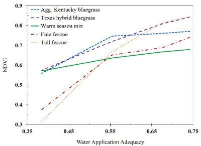
The range of variation in NDVI and SAVI was largest for TF, followed in order by FF, THB, AKB, and WSM. This means that Festuca species were the most sensitive and the mixture of warm season grasses was the most tolerant to water limitation.
(ii)
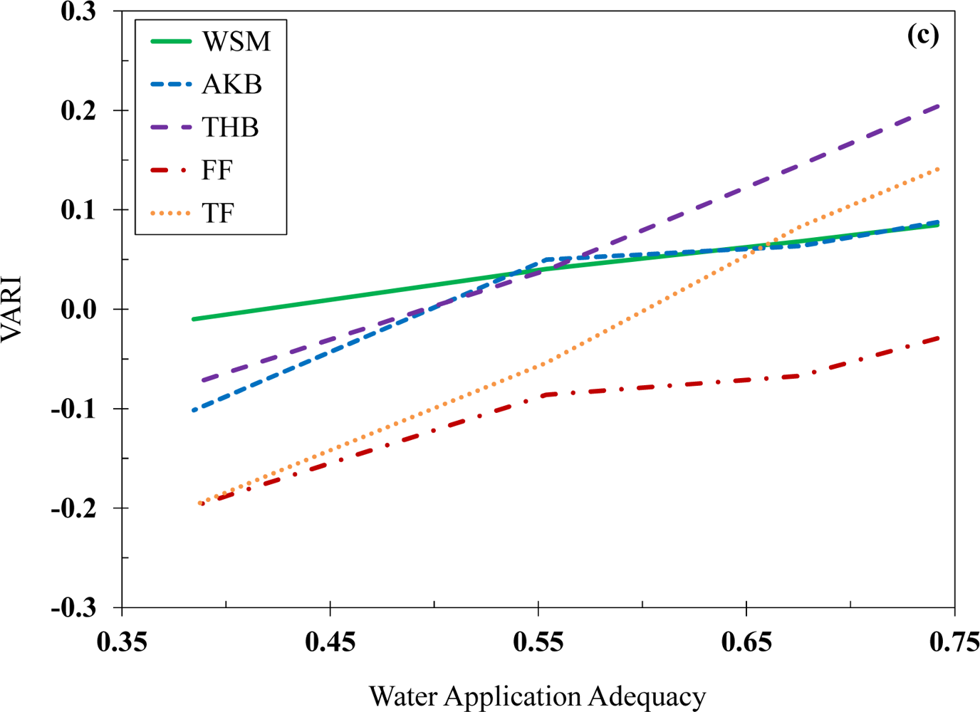
Except for the WSM plots, the NDVI-vs.-WAA and the SAVI-vs.-WAA relationships were non-linear, having different slopes at WAA levels below and above 0.55. In case of VARI, plots of WSM, THB, and TF appeared to have linear graphs, while other species demonstrated a non-linear pattern. Other studies have reported similar non-linear relationships between turfgrass quality indicators and water availability [8,40].
(iii)
Pairwise multiple comparison analysis (Holm-Sidak method) revealed that NDVI estimates at the two highest WAA levels were not statistically different. In comparison with the highest WAA (closest distance to sprinklers), NDVI values at the third highest WAA level were not significantly different for WSM, AKB, and THB. The difference was significant only for TF and FF. At the lowest WAA level (farthest distance), all turfgrass species had a NDVI that was statistically different that the values for the highest WAA level. SAVI estimates had a similar behavior, suggesting that considerable water conservation can be achieved before turfgrass quality is significantly degraded. This is similar to a previous finding that irrigation depths can be reduced by 15% at a golf course without affecting the turf quality [13].
(iv)
According to all VIs, the quality and growth of WSM was poorer under high WAA levels and better under low WAA level in comparison to other species.
(v)
Treatment S did not cause any significant variation in estimated VIs, with average NDVI, SAVI, and VARI values of 0.88, 0.65, and 0.23, respectively. Since WAA was 95% at this treatment, the mentioned values can be regarded as the upper limits that respected VIs can reach over a non-water-stressed Kentucky bluegrass turf under conditions similar to those of this experiment.
The observed sensitivity of remotely sensed turfgrass growth (NDVI and SAVI) and color (VARI) indicators to water availability suggests that these VIs can replace the traditional methods of visual quality assessment, which are time-consuming and subjective. For example, it seemed that all of the plots with an acceptable aesthetic appearance had a positive VARI during the study period. Thus, a VARI value of zero may be an appropriate threshold in managing turfgrass quality. The graphs in Figure 3 can also be used by turf managers to quantify the amount of reduction in applied water that can be achieved before turfgrass quality is degraded to a level lower than any desired VI.

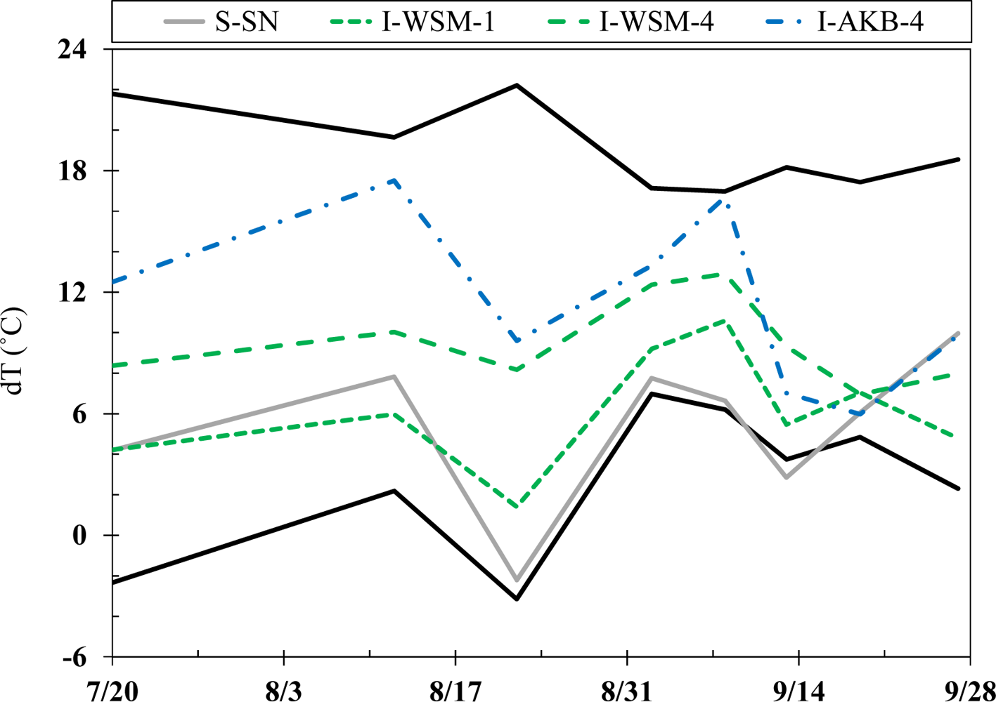
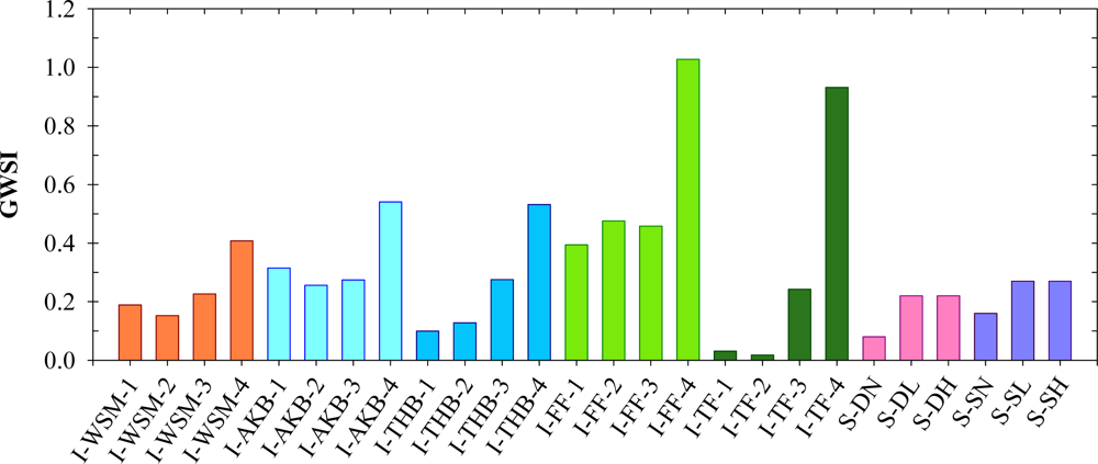
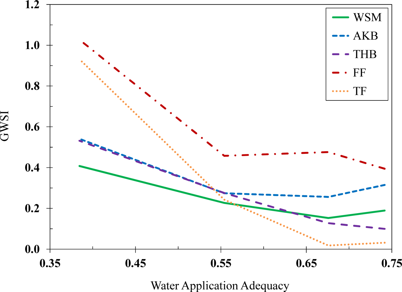
3.2. Grass Water Stress Index

Non-water-stressed baselines were developed for tall fescue and Kentucky bluegrass, following the methodology that was explained in previous sections. Developed relationships were essentially identical for both species, with a large coefficient of determination (R2 = 0.97):
dT LL = 3.3 ( VPD ) + 10.3
This similarity is contradictory to the findings of several previous studies that dTLL-VPD relationships are species-specific [21]. However, Carrow [41] stated that these baselines are similar enough to be combined for practical purposes such as irrigation scheduling. The slope of Equation (9) is a larger negative number compared to −2.2, which is the slope of similar equations developed for tall fescue [22] and Kentucky bluegrass [17]. This difference is most probably due to the difference in climatological conditions. Carrow [41] reported that non-water-stressed baselines developed for turfgrass species under arid/semi-arid climate had larger negative slopes compared to those developed under humid conditions.
The non-transpiring baseline was developed by entering the coefficients of Equation (9) into Equation (6). Predicted dTUL values varied from 17.0 to 21.9 °C, also bigger than the finding of Throssell et al. [17] who reported a dTUL value of about 13.0 °C for Kentucky bluegrass at an air temperature of 30.0 °C. However, dTUL values modeled in this experiment had a high accuracy when compared with dTm values that were measured over a non-transpiring turfgrass surface, with a mean bias error of only 0.7 °C and a root mean square error of 0.6 °C. Such a high accuracy suggests that observed differences in the upper and lower dT limits between this study and previous works is mainly due to differences in climatological conditions. It also suggests that the empirical GWSI approach can provide accurate results, if it is developed and applied locally under a high intensity of incoming solar radiation (around solar noon on cloud-free days). Figure 4 demonstrates the upper and lower dT limits, along with dTm values of four experimental plots as an example. According to this figure, dTm values for I-WSM-4 and I-AKB-4 plots that received minimum amounts of irrigation were closer to the dTUL line compared to the S-SN and I-WSM-1 plots.
The next step was to estimate GWSI over all experimental plots (Figure 5). For treatment S, different levels of added plant compost had no significant effect on water stress. Soil tillage depth did not have any significant effect either and there was no statistical interaction between these two factors (two-way ANOVA, P < 0.05). Within treatment I, the results showed that variations in WAA caused statistically significant (one-way ANOVA, P < 0.05) changes in GWSI for all studied turfgrass species (all datasets passed both equal variance and normality tests). However, the range of GWSI variation with WAA was not similar among turfgrass species. While the WSM and AKB varieties had the lowest GWSI range of 0.26 and 0.28, respectively, the difference between minimum and maximum GWSI values observed over the TF plot reached 0.91, close to the full possible range of unity. Therefore, the GWSI results based on the thermal remotely sensed data confirmed the VI results based on the optical remotely sensed data that the warm season grasses were the most tolerant and the Festuca species were the most sensitive species to water availability.
Similar to VIs results, turfgrass species had different responses at the same distances from sprinklers (i.e., for the same WAA levels). At the farthest location, FF had a GWSI of unity (Figure 6), followed by the GWSI of TF (0.93). Bluegrass species (AKB and THB) had the same GWSI values of 0.53. A similar GWSI value of about 0.50 is reported for Kentucky bluegrass under moderate levels of water stress (corresponding to a soil water potential of −0.40 MPa, measured by a gypsum resistance block installed at a soil depth of 76 mm) [17]. The smallest GWSI value (0.41) at this location belonged to WSM. This observation was expected because warm season grasses have a higher drought tolerance compared to cool season species. In addition, the two warm season species of this study are native in Colorado and therefore well-adapted to Colorado’s climate. At the closest location (largest WAA), however, TF out-performed other species with a negligible GWSI. THB had the next lowest GWSI (0.10), followed by that of WSM (0.19). The average GWSI was 0.15 for WSM at the second closest distance to sprinklers, where WAA was 68%. This result is very similar to the GWSI value of 0.16 that was estimated for bermudagrass (a warm season species) under a similar relative water use (actual to reference ET) of 66% [20].
Figure 6 also portrays that the GWSI-vs.-WAA relationship was non-linear, similar to the VIs-vs.-WAA relationships. Pairwise multiple comparison analyses (Holm-Sidak test, P < 0.05) revealed that within each turfgrass species, the differences in average GWSI for the three highest WAA levels (74, 68, and 55%) were not statistically significant. It was only the lowest WAA (38%) that caused a level of water stress that was significantly different than other WAA levels. Jalali-Farahani et al. [20] plotted GWSI values vs. percent available extractable water (AEW), defined as the ratio of the actual soil moisture minus the minimum amount of extractable water divided by the total extractable water. The generated GWSI-vs.-AEW scatterplots also showed a non-linear relationship, with GWSI increasing gradually from zero to 0.25 for the first 50% reduction in AEW and then increasing sharply until it reached unity.

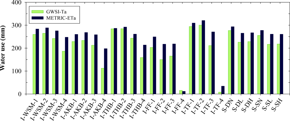
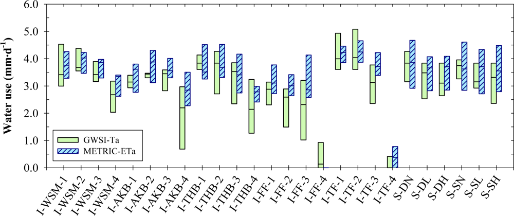
3.3. Turfgrass Water Use

3.3.1. GWSI-Based Water Use

Daily turfgrass Ta was calculated based on GWSI estimates for each of the seven dates of data collection. As expected, GWSI variations were translated into variations in Ta estimates. The highest water consumption rate was estimated over I-TF-1 and I-TF-2 plots (closest to the sprinklers), with average transpiration of 4.1 mm·d−1. The lowest water use rate also belonged to a TF plot (the farthest distance from sprinklers), with an average Ta of 0.2 mm·d−1. The Ta rates reached a maximum value of 3.4 mm·d−1 at AKB plots of treatment I, slightly smaller than the maximum Ta rate of 3.8 mm·d−1, estimated over the plots of treatment S that had the same type of turfgrass but received more irrigation water. Averaging Ta values over all WAA levels (distances from sprinklers) for each turfgrass species at treatment I showed that WSM had the highest average transpiration rate (3.3 mm·d−1), followed by THB (3.2 mm·d−1), AKB (2.9 mm·d−1), TF (2.9 mm·d−1), and FF (1.9 mm·d−1) species. This trend in Ta values agrees well with the observed trends in VIs. Average ETo estimated using the weather station data and the ASCE standardized Penman-Monteith method [32] was 4.5 mm·d−1 for the same seven data collection dates.

3.3.2. METRIC-Based Water Use

In general, the water use results obtained by applying the METRIC energy balance model were similar to those of the empirical GWSI approach. For example, I-TF-1 and I-TF-2 plots had the highest average METRIC-ETa rates of 4.3 mm·d−1. In addition, the average ETa for the I-TF-4 plot, which was the smallest based on the GWSI method, was the second smallest based on METRIC. The differences between the daily water use results of GWSI and METRIC methods were always less than 1.0 mm·d−1, with an average value of 0.4 mm·d−1 for all plots. This difference was 11% of the average METRIC-ETa for the same seven dates. Bastiaanssen et al. [42] reported that at field scale, the error in daily water use estimate of the land surface energy balance models can be up to 15%. A more recent study showed that on daily scales, the errors in METRIC results can be reduced to 10% if a surface roughness model is also incorporated to account for the surface heterogeneity [35]. Hence, the observed differences between GWSI and METRIC results in this study are well within the accuracy range of the METRIC model.
Statistical analyses were also performed to identify if there was any significant difference among the results of the METRIC and GWSI methods. As the first step, a normality test (Shapiro-Wilk) was conducted to select an appropriate group-comparison test. Databases that passed the normality test (P = 0.05) were analyzed using the un-paired t-test, while those that did not pass the test were analyzed using Mann-Whitney Rank Sum test. The results confirmed that the difference between two methods was not statistically significant (P > 0.05) for any of the studied plots. A similar observation was reported when the same two methods were applied to estimate water consumption of corn in northeastern Colorado [38]. This finding is of great importance, since METRIC is a complex and data-intensive model that needs to be applied by a trained operator. The empirical approach of GWSI, however, is an easy-to-apply method that neither requires an extensive knowledge on land surface processes nor needs extensive data collection and processing. In addition, the procedure can be easily programmed in pocket computers and smart phones. There is also the possibility of applying the GWSI approach to air- and space-borne imagery. This method does not rely on optical remote sensing data, only a single-layer map of radiometric surface temperature suffices for its application. However, GWSI method is only as accurate as the baselines used in defining the lower and upper limit of dT. These baselines need to be developed under the specific conditions of each climatic region, so they are not transferable among the regions. Surface energy balance models, on the other hand, can be applied over large areas comprising different vegetation types, regardless of climatic conditions.
Figure 7 demonstrates box plots of estimated Ta and ETa, averaged for all data collection dates. As this figure suggests, the range and median of turfgrass water use estimates were similar among both methods, except for the two farthest locations from the sprinklers in treatment I. In other words, the difference between water use estimates of GWSI and METRIC methods had a negative relationship with the depth of applied water (or the WAA level). This is most probably due to the fact that at lower WAA levels (farther distances from sprinklers) turfgrass canopy was not fully closed. Hence, parts of the underlying soil may have been viewed by the IRT, despite our effort to take readings only over turfgrass. This would have contaminated the measured turfgrass temperatures, resulting in larger GWSI and consequently smaller Ta estimates. The difference between GWSI and METRIC results was reduced from 11% to 8%, when only the higher-quality plots (those that had a positive VARI) were included in the analysis.
A traditional approach in estimating the water requirement of non-water-stressed agricultural crops is to obtain the so-called crop coefficients (Kc) for each growth stage of the crop under consideration and then multiply these coefficients by the reference ET. Due to its widespread application, Kc values are reported for major agricultural crops and turfgrass species in publications such as the FAO paper 56. According to the tables in FAO paper 56, mid-season Kc is 0.87 and 0.97 for warm season and cool season turfgrass, respectively, after adjustment are made to account for the arid/semi-arid climate of the study area [31]. In this study, turfgrass Kc values were obtained through dividing the METRIC-ETa by the ETo. The average METRIC-Kc at the closest distance to the sprinklers (non-water-stressed) was 0.86 over WSM and 0.98 over TF, very similar to the values proposed in the FAO paper 56. The FAO paper 56 also outlines a procedure for estimating a stress coefficient (Ks), which reduces the actual water use estimate in proportion to the experienced soil water deficit in the root zone of studied plant.
Daily values of water use based on both METRIC and GWSI methods were interpolated for the days in between remote sensing data acquisition dates and then summed to provide an estimate of the cumulative water consumption for the entire seventy days of study. The results had a pattern similar to that of daily values, with a total water use that ranged from 8 to 300 mm based on GWSI and from 12 to 321 mm based on METRIC (Figure 8). Grass reference ET was 329 mm during the same period. For both average daily and cumulative water use estimates, it should be noted that uncertainties associated with sensors, methods, and assumptions propagate to the final approximations. Further studies are required to address the error propagation and the sensitivity of each model (especially the GWSI) to uncertainties in input variables.

4. Conclusions

Ground-based optical and thermal remote sensing data were used to study the quality, water stress, and water consumption of several turfgrass species under different soil and irrigation treatments in northern Colorado, USA. Reducing water application from 74% to 38% of the total grass-based reference ET resulted in average NIR reflectance to decrease from 38% to 28%, while the SWIR reflectance increased from 25% to 35%. Reflectance in the visible bands also experienced about a twofold increase. Measured surface reflectance in multiple wavebands was used to estimate three vegetation indices (VIs), namely NDVI, SAVI, and VARI. Utilizing the simple empirical approach of estimating grass water stress index (GWSI) was also investigated. Similar non-water-stressed baselines were developed for tall fescue and Kentucky bluegrass species. The modeled estimates of non-transpiring turfgrass temperature had a small error (0.7 °C) when compared to the temperature readings taken over a non-transpiring patch of turfgrass. All optical (three VIs) and thermal (GWSI) indicators were consistent in having a non-linear relationship with water application depth. They also revealed that Festuca species were the most sensitive and warm season species were the least sensitive to water limitation.
The difference between turfgrass water use estimates based on GWSI and METRIC methods was not statistically significant, suggesting that GWSI can be used for identifying both the timing and amount of irrigation events. This difference was 0.4 mm·d−1 on average, which was 11% of the METRIC-based estimates and smaller than the expected error of METRIC model when applied at field scale (15%). The range of cumulative water use estimates for all experimental plots was 8–300 mm and 12–321 mm based on GWSI and METRIC methods, respectively. METRIC-based crop coefficients for non-water-stressed plots were similar to tabulated values reported in the FAO paper 56, being 0.86 and 0.98 for warm season and cool season turfgrass, respectively. More studies need to be conducted to include several growing seasons, as yearly variation in climatological conditions could have a significant effect on turfgrass response to different soil and irrigation treatments.

Acknowledgments

This research was funded by the Northern Colorado Water Conservancy District. Funding for open access to the article was provided by the Colorado State University Libraries Open Access Research and Scholarship Fund. The authors would like to express their appreciation to Abhinaya Subedi for his assistance in data collection.
  • Conflict of InterestThe authors declare no conflict of interest.

References and Notes

  1. Boland, J.J. Assessing urban water use and the role of water conservation measures under climate uncertainty. Climatic Change 1997, 37, 157–176. [Google Scholar]
  2. Kjelgren, R.; Rupp, L.; Kilgren, D. Water conservation in urban landscape. HortScience 2000, 35, 1037–1040. [Google Scholar]
  3. Cooley, H.; Gleick, P.H. Urban Water-Use Efficiencies: Lessons from United States Cities. In The World’s Water 2008–2009: The Biennial Report on Freshwater Resources; Gleick, P.H., Ed.; Island Press: Washington, DC, USA, 2009; pp. 101–122. [Google Scholar]
  4. Hilaire, R.S.; Hall, S.; Cruces, L.; Arnold, M.A.; Wilkerson, D.C.; Devitt, D.A.; Hurd, B.H.; et al. Efficient water use in residential urban landscapes. HortScience 2008, 43, 2081–2092. [Google Scholar]
  5. Wu, J.; Bauer, M.E. Estimating net primary production of Turfgrass in an urban-suburban landscape with QuickBird imagery. Remote Sens. 2012, 4, 849–866. [Google Scholar]
  6. Carrow, R.N. Turfgrass Irrigation Scheduling by Infrared Thermometry. Proceedings of the 1989 Georgia Water Resources Conference, Athens, GA, USA, 16–17 May 1989; pp. 63–65.
  7. Bell, G.E.; Martin, D.L.; Wiese, S.G.; Dobson, D.D.; Smith, M.W.; Stone, M.L.; Solie, J.B. Vehicle-mounted optical sensing: An objective means for evaluating turf quality. Crop Sci. 2002, 42, 197–201. [Google Scholar]
  8. McKenney, C.B.; Zartman, R.E. Response of Buffalograss and Bermudagrass to reduced irrigation practices under semiarid conditions. J. Turf. Manag. 1997, 2, 45–54. [Google Scholar]
  9. Trenholm, L.E.; Schlossberg, M.J.; Lee, G.; Parks, W.; Geer, S.A. An evaluation of multi-spectral responses on selected turfgrass species. Int. J. Remote Sens. 2000, 21, 709–721. [Google Scholar]
  10. Martin, D.L.; Wehner, D.J.; Throssell, C.S.; Fermanian, T.W. Evaluation of four crop water stress index models for irrigation scheduling decisions on Penncross Creeping Bentgrass. Int. Turf Soc. Res. J. 2005, 10, 373–386. [Google Scholar]
  11. Fitz–Rodríguez, E.; Choi, C.Y. Monitoring turfgrass quality using multispectral radiometry. Trans. ASAE 2002, 45, 865–871. [Google Scholar]
  12. Baghzouz, M.; Devitt, D.A.; Morris, R.L. Evaluating temporal variability in the spectral reflectance response of annual ryegrass to changes in nitrogen applications and leaching fractions. Int. J. Remote Sens. 2006, 27, 4137–4157. [Google Scholar]
  13. Bastug, R.; Buyuktas, D. The effects of different irrigation levels applied in golf courses on some quality characteristics of turfgrass. Irrig. Sci. 2003, 22, 87–93. [Google Scholar]
  14. Fenstermaker-Shaulis, L.K.; Leskys, A.; Devitt, D.A. Utilization of remotely sensed data to map and evaluate turfgrass stress associated with drought. J. Turf. Manag. 1997, 2, 65–81. [Google Scholar]
  15. Park, D.M.; Cisar, J.L.; Williams, K.E.; McDermitt, D.K.; Miller, W.P.; Fidanza, M.A. Using spectral reflectance to document water stress in Bermudagrass grown on water repellent sandy soils. Hydrol. Process. 2007, 21, 2385–2389. [Google Scholar]
  16. Johnsen, A.R.; Horgan, B.P.; Hulke, B.S.; Cline, V. Evaluation of remote sensing to measure plant stress in Creeping Bentgrass (L.) fairways. Crop Sci. 2009, 49, 2261–2274. [Google Scholar]
  17. Throssell, C.S.; Carrow, R.N.; Milliken, G.A. Canopy temperature-based irrigation scheduling indices for Kentucky Bluegrass turf. Crop Sci. 1987, 27, 126–131. [Google Scholar]
  18. Jackson, R.D.; Idso, S.B.; Reginato, R.J. Canopy temperature as a crop water stress indicator. Water Resour. Res. 1981, 17, 1133–1138. [Google Scholar]
  19. Idso, S.B.; Jackson, R.D.; Pinter, P.J., Jr.; Reginato, R.J.; Hatfield, J.L. Normalizing the stress-degree-day parameter for environmental variability. Agric. Meteorol. 1981, 24, 45–55. [Google Scholar]
  20. Jalali-Farahani, H.R.; Slack, D.C.; Kopec, D.M.; Matthias, A.D. Crop water stress index models for Bermudagrass turf: a comparison. Agron. J. 1993, 85, 1210–1217. [Google Scholar]
  21. Martin, D.L.; Wehner, D.J.; Throssell, C.S. Models for predicting the lower limit of the canopy-air temperature difference of two cool season grasses. Crop Sci. 1994, 34, 192–198. [Google Scholar]
  22. Al-Faraj, A.; Meyer, G.E.; Horst, G.L. A crop water stress index for tall fescue (Festuca arundinacea Schreb.) irrigation decision-making—A traditional method. Comput. Electron. Agr. 2001, 31, 107–124. [Google Scholar]
  23. Payero, J.O.; Neale, C.M.U.; Wright, J.L. Non-water-stressed baselines for calculating crop water stress index (CWSI) for alfalfa and tall fescue grass. Trans. ASAE 2005, 48, 653–661. [Google Scholar]
  24. Idso, S.B. Non-water-stressed baselines: A key to measuring and interpreting plant water stress. Agric. Meteorol. 1982, 27, 59–70. [Google Scholar]
  25. CropScan. Available online: http://www.cropscan.com/ (accessed on 12 November 2012).
  26. Deering, D.W. Rangeland Reflectance Characteristics Measured by Aircraft and Spacecraft Sensors. Ph.D. Dissertation, Texas A & M University, College Station, TX, USA. 1978. [Google Scholar]
  27. Huete, A.R. A soil-adjusted vegetation index (SAVI). Remote Sens. Environ. 1988, 25, 295–309. [Google Scholar]
  28. Gitelson, A.A.; Stark, R.; Grits, U.; Rundquist, D.; Kaufman, Y.; Derry, D. Vegetation and soil lines in visible spectral space: A concept and technique for remote estimation of vegetation fraction. Int. J. Remote Sens. 2002, 23, 2537–2562. [Google Scholar]
  29. Baghzouz, M.; Devitt, D.A.; Morris, R.L. Assessing canopy spectral reflectance of hybrid Bermudagrass under various combinations of nitrogen and water treatments. Appl. Eng. Agric. 2007, 23, 763–774. [Google Scholar]
  30. Allen, R.G.; Tasumi, M.; Trezza, R. Satellite-based energy balance for mapping evapotranspiration with internalized calibration (METRIC)-model. J. Irrig. Drain. Eng. 2007, 133, 380–394. [Google Scholar]
  31. Allen, R.G.; Pereira, L.S.; Raes, D.; Smith, M. Crop Evapotranspiration: Guidelines for Computing Crop Requirements; Irrigation and Drainage Paper No. 56; FAO: Rome, Italy, 1998. [Google Scholar]
  32. ASCE-EWRI. The ASCE Standardized Reference Evapotranspiration Equation. Report by the American Society of Civil Engineers Task Committee on Standardization of Reference Evapotranspiration; Allen, R.G., Walter, I.A., Elliot, R.L., Howell, T.A., Itenfisu, D., Jensen, M.E., Snyder, R.L., Eds.; ASCE: Reston, VA, USA, 2005. [Google Scholar]
  33. Brest, C.L.; Goward, S.N. Driving surface albedo measurements from narrow band satellite data. Int. J. Remote Sens. 1987, 8, 351–367. [Google Scholar]
  34. Bastiaanssen, W.G.M.; Menenti, M.; Feddes, R.A.; Holtslang, A.A. A remote sensing surface energy balance algorithm for land (SEBAL): 1. Formulation. J. Hydrol. 1998, 212–213, 198–212. [Google Scholar]
  35. Chávez, J.; Gowda, P.; Howell, T.; Garcia, L.; Copeland, K.; Neale, C. ET Mapping with high-resolution airborne remote sensing data in an advective semiarid environment. J. Irrig. Drain. Eng. 2012, 138, 416–423. [Google Scholar]
  36. Chávez, J.L.; Neale, C.M.U.; Prueger, J.H.; Kustas, W.P. Daily evapotranspiration estimates from extrapolating instantaneous airborne remote sensing ET values. Irrig. Sci. 2008, 27, 67–81. [Google Scholar]
  37. Colaizzi, P.D.; Evett, S.R.; Howell, T.A.; Tolk, J.A. Comparison of five models to scale daily evapotranspiration from one-time-of day measurements. Trans. ASABE 2006, 49, 1409–1417. [Google Scholar]
  38. Taghvaeian, S.; Chávez, J.L.; Hansen, N.C. Infrared thermometry to estimate crop water stress index and water use of irrigated maize in Northeastern Colorado. Remote Sens. 2012, 4, 3619–3637. [Google Scholar]
  39. Tucker, C.J. Remote sensing of leaf water content in the near infrared. Remote Sens. Environ. 1980, 10, 23–32. [Google Scholar]
  40. Feldhake, C.M.; Danielson, R.E.; Butler, J.D. Turfgrass evapotranspiration. II. Responses to deficit irrigation. Agron. J. 1984, 76, 85–89. [Google Scholar]
  41. Carrow, R.N. Canopy temperature irrigation scheduling indices for turfgrasses in humid climate. In International Turfgrass Society Research Journal 7; Carrow, R.N., Christians, N.E., Shearman, R.C., Eds.; Intertec Publishing Corp: Overland Park, KS, USA, 1993; pp. 594–599. [Google Scholar]
  42. Bastiaanssen, W.G.M.; Noordman, E.J.M.; Pelgrum, H.; Davids, G.; Thoreson, B.P.; Allen, R.G. SEBAL model with remotely sensed data to improve water-resources management under actual field conditions. J. Irrig. Drain. Eng. 2005, 131, 85–93. [Google Scholar]
Figure 1. Aerial false color image of the study site (Conservation Gardens at Northern Water) and its location in northern Colorado, USA. Treatments I and S and the weather station (WS) locations are identified in this image.
Remotesensing 05 02327f1
Figure 2. Spectral signatures of turfgrass species under two different irrigation application rates: (a) 13 mm·h−1 and (b) 5 mm·h−1 and averaged for all measurement dates.
Remotesensing 05 02327f2
Figure 3. Effect of water application adequacy on (a) NDVI, (b) SAVI, and (c) VARI, averaged for all measurement dates.
Remotesensing 05 02327f3aRemotesensing 05 02327f3b
Figure 4. Modeled dTLL (lower solid black lines) and dTUL (upper solid black lines), along with dTm values for four experimental plots.
Remotesensing 05 02327f4
Figure 5. Average GWSI for all of the experimental plots.
Remotesensing 05 02327f5
Figure 6. Variations in GWSI with changes in water application adequacy.
Remotesensing 05 02327f6
Figure 7. Box-plots of estimated turfgrass water use based on GWSI and METRIC methods for all measurement dates.
Remotesensing 05 02327f7
Figure 8. Total turfgrass water use during the study period (70 days) based on GWSI and METRIC methods.
Remotesensing 05 02327f8
Table 1. Key weather variables during the study period (20 July–27 September 2011).
ParameterValueUnits
Average daily minimum air temp.12.6°C
Average daily mean air temp.20.9°C
Average daily maximum air temp.29.3°C
Average daily mean wind speed1.5m·s−1
Average daily vapor pressure1.1kPa
Average daily solar radiation20.6MJ·d−1
Total precipitation54.0mm
Average daily ETo4.7mm·d−1
Total ETo329.0mm
Table 2. Experimental plots, abbreviations, and total irrigation water applied during the study period (20 July–27 September 2011).
TreatmentExperimental plotsAbb.Irr. (mm)
Irrigation depth (I)Warm Season Mix, 1.0*I-WSM-1190
Warm Season Mix, 2.1I-WSM-2169
Warm Season Mix, 3.3I-WSM-3129
Warm Season Mix, 4.5I-WSM-473
Agg. Kent. Bluegrass, 1.0I-AKB-1190
Agg. Kent. Bluegrass, 2.1I-AKB-2169
Agg. Kent. Bluegrass, 3.3I-AKB-3129
Agg. Kent. Bluegrass, 4.5I-AKB-473
Texas Hyb. Bluegrass, 1.0I-THB-1190
Texas Hyb. Bluegrass, 2.1I-THB-2169
Texas Hyb. Bluegrass, 3.3I-THB-3129
Texas Hyb. Bluegrass, 4.5I-THB-473
Fine Fescue, 1.0I-FF-1190
Fine Fescue, 2.1I-FF-2169
Fine Fescue, 3.3I-FF-3129
Fine Fescue, 4.5I-FF-473
Tall Fescue, 1.0I-TF-1190
Tall Fescue, 2.1I-TF-2169
Tall Fescue, 3.3I-TF-3129
Tall Fescue, 4.5I-TF-473

Soil Preparation (S)Deep tillage, No compostS-DN259
Deep tillage, Low compostS-DL259
Deep tillage, High compostS-DH259
Shallow tillage, No compostS-SN259
Shallow tillage, Low compostS-SL259
Shallow tillage, High compostS-SH259
*Distance from line-source sprinklers (m).

