Topographic Correction of Wind-Driven Rainfall for Landslide Analysis in Central Taiwan with Validation from Aerial and Satellite Optical Images

Abstract

Rainfall intensity plays an important role in landslide prediction especially in mountain areas. However, the rainfall intensity of a location is usually interpolated from rainfall recorded at nearby gauges without considering any possible effects of topographic slopes. In order to obtain reliable rainfall intensity for disaster mitigation, this study proposes a rainfall-vector projection method for topographic-corrected rainfall. The topographic-corrected rainfall is derived from wind speed, terminal velocity of raindrops, and topographical factors from digital terrain model. In addition, scatter plot was used to present landslide distribution with two triggering factors and kernel density analysis is adopted to enhance the perception of the distribution. Numerical analysis is conducted for a historic event, typhoon Mindulle, which occurred in 2004, in a location in central Taiwan. The largest correction reaches 11%, which indicates that topographic correction is significant. The corrected rainfall distribution is then applied to the analysis of landslide triggering factors. The result with corrected rainfall distribution provides better agreement with the actual landslide occurrence than the result without correction.

1. Introduction

Rainfall is a major factor triggering landslides in Taiwan, and the intensity of rain plays an essential role in the landslide prediction. However, the influence of topography in the rainfall direction and intensity is usually neglected in the analysis of the relations between rainfall amount or intensity and landslide occurrence. There is no differentiation between rainfall on windward slopes and on leeward slopes. Because rainfall always occurs together with strong winds in a typhoon event, there is consistently strong horizontal wind momentum with changing directions. The need for adjusting rainfall distribution for the topographic effect seems essential.

Landslides are massive earth movements caused by gravity and frequently triggered by factors such as rainfall. Various types of remote sensing tools are extensively applied in understanding both landslides factors and feature recognition for landslide susceptibility [1–6]. Rainfall is the most important triggering factor in Taiwan due to its tropical and sub-tropical climate. The studies of De Lima [7], Helming [8], and Sharon [9] all recognized that using vertical rainfall alone is not sufficient for describing rainfall effects on slope soil erosion, since wind speed and wind direction should also be considered. The force component normal to the slope is identified as the most important contributing factor to rainfall splash on soil surface. Similarly, vertical rainfall is not sufficient to describe the rainfall effects on unconsolidated overburdens of shallow landslides. Schulz [10,11] observed that most landslides in Seattle might not be caused by ground-water conditions especially those triggered by heavy precipitation. In addition, the aspect of a slope will not only dominate the impact angle of a raindrop but also the intensity of the rainfall. As shown in Figure 1, total rain-drops (N) collected with a rain gauge of area A in any location within a plain area (Figure 1(a)) are the same. However, in a sloping area, the leeward side is subjected to lower rainfall intensity than the windward side (Figure 1(b)). Thus, the topographic effects should be considered in the rainfall estimation.

Taiwan is located in tropical and sub-tropical zones, and often suffers from heavy rainfall, especially during typhoons. In addition, Taiwan is located at a tectonic suture zone, with collisions occurring between the Philippine Sea and Eurasian plates. More than 70% of Taiwan is covered by mountainous terrain, with rock formations highly fractured and jointed. These physiographic settings make Taiwan a fragile land, especially vulnerable to rainfall-induced landslides. As an example, 106 landslides with an area of 1,290,745 m² were observed and reported in the Alishan watershed with total area of 36 km²[12]. About 4% of this area is covered by landslides.

For practical applications in the physiographic environments of Taiwan, the classification scheme of landslides developed by Varnes [13] is simplified into five major categories, namely, rock falls, shallow-seated landslides, deep-seated landslides, dip-slope and wedge slides, and debris flows, as shown in

Table 1. Simplified classification landslide scheme applied to Taiwan.

Type of Movements		Type of Materials
		Bed Rock	Engineering Soils
			Debris	Soils
Falls		Rock falls	Shallow-seated slide
Topples
Slide	Translational	Dip-slope and wedge slide
	Rotational	Deep-seated slide
Flows		(not applicable)	Debris flow	(not applicable)

. Types of landslides can be differentiated by their physical appearance, which is especially useful for applications with remotely sensed images.

Remote sensing is a useful tool for deriving landslide inventory [2,3,5,6,14–16], and the physical appearance of landslides is the basis of boundary recognition and landslide type. However, displaced materials of a rainfall-induced landslide are usually washed away from steep slopes, so only the fresh scars of the rupture surface remain. Fresh landslide scars emplaced at various slope gradients and locations normally include the following types, rock falls, debris slides, channel bank failures, and debris flows. Table 1 is a classification scheme used by Central Geological Survey, Taiwan [17]. In this study, the landslides of concern include all types of shallow-seated landslides, except debris flows. This exception is made because debris flows are triggered by a different mechanism, with more contributions from flowing water instead of gravity. In other words, debris flows are treated as a transformation of other shallow-seated landslides when high rainfall concentration and liquefaction of displaced materials take place.

Several researchers have reported that the rainfall intensity is an essential factor of rainfall-triggered landslide [18–20]. However, relatively few studies discussed the interpolation of rainfall intensity which employs topographic information. Thus, the objective of this study is to investigate topographic effects of rainfall interpolation with a case study from Central Taiwan after Typhoon Mindulle in 2004.

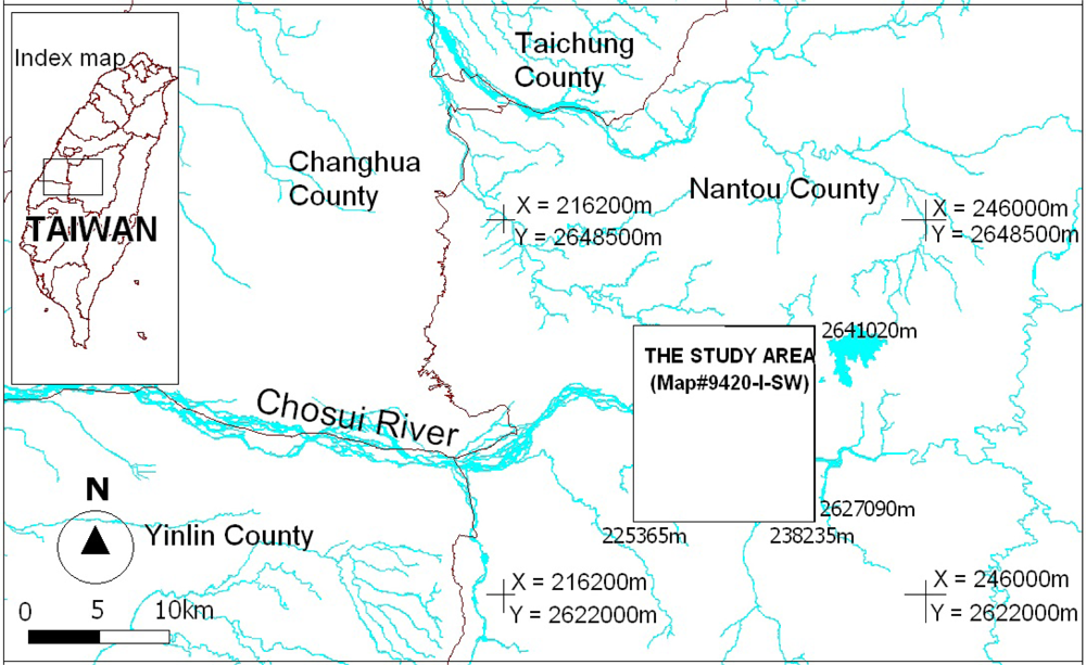
2. Study Area and Rainfall Event for an Experiment

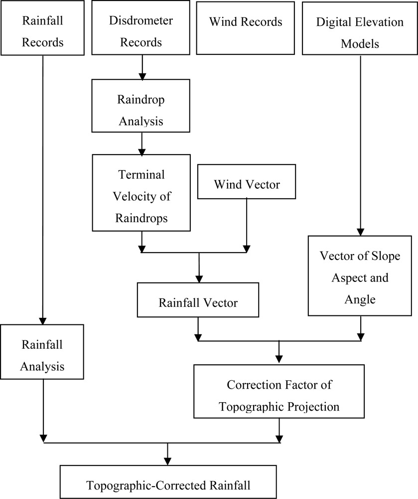
The study area is located in Nantou County, central Taiwan (Figure 2). This area is included in map number 95201SW in the national map series. The area covers 12,816 m in the east-west direction and 13,901 m in the north-south direction. The terrain has a very high relief. Rock formations are highly fractured due to the active mountain-building processes prevailing in Taiwan.

The event considered in this study is Typhoon Mindulle of 1–4 July 2004. Rainfall intensities recorded in the study area were as high as 110 mm/h at Suili Station, 120 mm/h at Jiji station, and 100 mm/h at Senlong Station. This was an “extreme torrential rain” according to Central Weather Bureau [21], with heavy rain in the central and southern parts of Taiwan. Many places in Central and Southern Taiwan received more than 1,000 mm of rainfall. The maximum wind speed in the typhoon center reached 45 m/s.

3. Methodology

Figure 3 shows the procedure for deriving topographic-corrected rainfall. Rainfall and wind datasets were collected from the Central Weather Bureau of Taiwan for periods before and after Typhoon Mindulle. In addition, raindrop analysis was based on the records of disdrometers [22]. Horizontal wind field and terminal raindrop velocity are combined to derive rainfall vectors. According to terrain aspect, the rainfall vector is further projected as a correction factor to account for topographic effects.

The rainfall vector is composed of wind speed and terminal velocity of raindrops, and projection of a rainfall vector onto a ground surface defines the amount of topographic correction needed. Wind speed vectors are deduced from wind records from weather stations. Terminal velocity of raindrops is derived from either raindrop distribution recorded by disdrometer or a specific rainfall pattern inference of the dedicated rainfall event. Subsequently, the projected rainfall vector of each grid cell is deduced employing a digital terrain model. Original rainfall distribution in the area is then adjusted with this correction.

The following section provides the details of the proposed scheme.

3.1. Determining the Terminal Velocity of Raindrops

A rainfall vector is composed of a wind vector and a terminal raindrop velocity. The hourly wind direction averages in degree from azimuth 0° to 360° and wind speeds in meters per second (m/s) are recorded in a standard weather station. Weather records of hourly rainfall and wind directions are acquired from Central Weather Bureau for all the 10 stations in Figure 2. Therefore, the derivation of wind vectors is straightforward. The hourly rainfall terminal velocity of the study area is obtained by the measurements of a 2D-video disdrometer [23].

Rainfall terminal velocity can be obtained from direct measurements [24,25] or derived from the raindrop spectrum of a Doppler Weather Radar [26]. It is generally recognized that terminal velocity and raindrop size are closely related [24,27]. Terminal velocity can be expressed as a function of raindrop size. Therefore, drop size distribution (DSD) is the key for deriving terminal velocity. DSD could be obtained from rainfall simulators [28–31] or from measurements of impact or optical disdrometers [32] or profilers. It is reported that DSD in Taiwan is dominated by rainfall types and seasonal changes [27,33].

The terminal velocity is derived from the mean value (D₀) of hourly average and Equation (1) [24]. Because DSD is both site and event dependent, V of Equation (1) will be site and event dependent, too. For the study area in middle Taiwan, the mean value (D₀) of the raindrop size is 1.8 mm for Typhoon Mindulle event. Therefore, the terminal velocity is 6.14 m/s.

$$\begin{array}{c}V=0.057D^3-0.9084D^2+4.9751D-0.2037\\ R^2=0.9998\end{array}$$

(1)

where:

V	the terminal velocity (m/s),
D	the raindrop size (mm),
R	the regression coefficient.

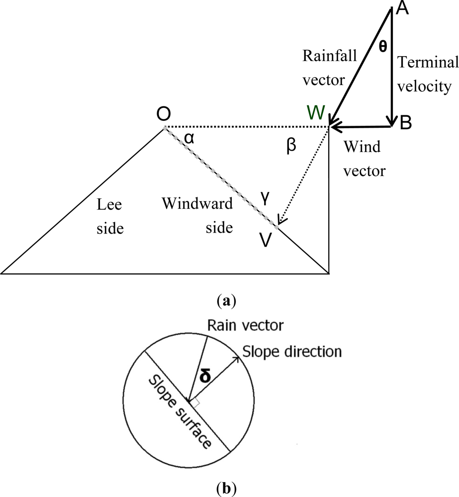
3.2. Determining the Wind Vector

A wind vector can be decomposed into east-west (abbreviated as E-W) and north-south (abbreviated as N-S) components. The hourly E-W and N-S components of each weather station are computed from the wind records. Subsequently, interpolation is performed with the irregularly distributed observations from scattered weather stations into regular grid for E-W and N-S components separately. Wind vectors of each grid cell are then derived from E-W and N-S components in each corresponding cell. Because the horizontal wind field is applied, the directions for the Mindulle event vary from azimuth 0 to 359 degrees with prevailing direction of 180–270 degrees. The magnitude of the average wind vectors during Typhoon Mindulle event range from 2.0 to 5.0 m/s.

3.3. Determine the Rainfall Vector

The correction factor for each grid cell in a dedicated rainstorm event could be derived with the following parameter sets:

• (a). the average rainfall vector of the highest 24-h rainfall intensity;
• (b). the accumulated rainfall vector of hourly average rainfall vectors in the highest 24-h rainfall intensity;
• (c). the average rainfall vector of the 12 h prior to the peak intensity of the event;
• (d). the accumulated rainfall vector of the hourly average rainfall vectors in the 12 h prior to the peak intensity of the event; and,
• (e). the accumulated rainfall vector of the hourly average rainfall vectors in the all hours of the event.

Which parameter set best describes the rainfall events remains for further study. Landslides are supposedly triggered when the ground soil becomes saturated and the most significant time is while rainfall intensity reaches its maximum. Therefore, (c) is adopted in this research though it might not be the best one.

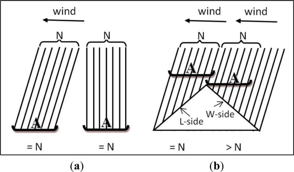
3.4. Determining the Correction Factor of Topographic Projection

A correction factor can be derived from the projection of the rainfall vectors onto the sloping ground surface, including the major factors of surface slope, aspect, and rainfall direction. Figure 4 illustrates the rainfall vector in relation to raindrop terminal velocity and horizontal wind speed. The key mechanism of topographic effect on rainfall intensity is the horizontal wind field. It is assumed that no significant turbulent winds or raindrop capture took place. Thus, actual rainfall received on a sloping surface should be corrected with the projection of the rainfall vector on the slope surface. The number of raindrops received on a windward sloping area is different from those on the leeside.

A digital elevation model is used as a spatial reference for computing the correction factor of each cell following the procedures shown in Figure 3. In each cell, rainfall vectors are derived from the slope azimuth, slope angle, wind vector, and terminal velocity of the corresponding cell in the same location. In the complete study area, the deviation of the rainfall vectors from the vertical ranges from 14.45° to 34.19°. Complete coverage of the correction factor (Kt) was then computed with the deviation angle of each grid cell with respect to the slope aspect. As shown in Figure 4(a), a unit distance OW in a horizontal plane is projected onto a windward slope with a distance of OV, where OV can be defined by deviation angle of θ, slope aspect α, and the unit distance OW. The rainfall on OW is received by the area of OV. Thus, if rainfall vector is normal to slope surface, the correction factor Kt′ is the ratio of OW to OV, as shown in Figure 4(a). Otherwise, a correction of azimuthal deviation (δ) has to be made, as shown in Figure 4(b). Therefore, the correction factor (Kt) is a function of theta (θ), alpha (α), and difference of azimuth angle of the slope and rain vector (δ), following Equation (2–4). As shown in Figure 4(b), because rainfall vectors may not be in the direction of slope dip direction, an azimuthal correction to the deviation of theta (δ) is thus applied as Equation (4):

$$\begin{array}{l}\because \text{Sine}\hspace{0.17em}\text{Law}:\text{OV}=\text{OW}(\text{sin}\beta /\text{sin}\left(\alpha +\beta \right)\\ \hspace{0.17em}\hspace{0.17em}\hspace{0.17em}\hspace{0.17em}\hspace{0.17em}\hspace{0.17em}\hspace{0.17em}\hspace{0.17em}\hspace{0.17em}\hspace{0.17em}\hspace{0.17em}\hspace{0.17em}\hspace{0.17em}\hspace{0.17em}\hspace{0.17em}\hspace{0.17em}\hspace{0.17em}\text{and}\beta =90°-\theta \end{array}$$

(2)

$$\because \text{K}{\text{t}}^{\prime }=\frac{\text{OW}}{\text{OV}}=\frac{\text{sin}\left(\alpha +90°-\theta \right)}{\text{sin}\left(90°-\theta \right)}$$

(3)

$$\text{Kt}=\text{K}{\text{t}}^{\prime }\text{cos}(\delta )$$

(4)

3.5. Kernel Density Analysis of Landslides

Landslide occurrence with respect to a certain factor can be presented with a statistical table describing the fractions of each attribute class. The ordinate axis is the frequency and the abscissa axis is the attribute classes. This could be presented with a scatter plot as well. As shown in Figure 5(a), each landslide that occurred after the typhoon event is plotted as a point with the slope on the vertical axis and rainfall on the horizontal axis. Clusters of points indicate concentration of landslide occurrences. The scatter plot could be further processed with kernel density estimation, as shown in Figure 5(b). Kernel density is a nonparametric way to estimate the probability density function for a given variable [34]. Unlike histograms, kernel densities do not group data into bins, but use small bumps estimated by the kernel function. Instead of a simple mathematical division of the area covered by landslides of the total study area, kernel density estimation produces a map of smoothed continuous intensity estimation. Compared with a histogram, the interactions of two parameters such as slope and rainfall could be visualized, which improves the perception of the controlling factors.

Kernel density estimation (KDE) is applied to process the dispersed discrete point features [34–36] and provide a better representation of the features under combined effects. The result of a KDE is usually a raster dataset where each cell has a density value that is weighted according to distance from the starting features. The user can choose the cell size of the output raster, the attribute field to be used in the calculation, its units of measure, and the search radius.

A density map is an exploratory spatial analysis tool to visualize the trend of a point pattern. A smoothed density map is a continuously varying surface where each grid represents the density of the underlying point process and it offers a quick overview of the spatial pattern of the point events. Such a map can be calculated by overlaying the event datasets with a grid and calculating the event density, D, within a search region with radius, h, around the center of every grid cell. A kernel function is used to fit a smoothly tapered surface to each point and the density is calculated from the surfaces where they overlap the center of the output grid cell. This gives a smoother output grid, while maintaining the same general values for density.

Density values vary according to the software used [36]. The quadratic kernel function implemented in ESRI ArcGIS 9.1© with the Spatial Analyst© extension was used. The function takes the following form:

$$D\left(s\right)=\{\begin{array}{cc}\sum _{i=1}^n{s}_i\left(\frac{3}{\pi {\tau }^2}\right){\left[1-\left(\frac{h_i}{{\tau }^2}\right)\right]}^2,& h_i<\tau \\ 0,& h_i\ge \tau \end{array}$$

(5)

where:

τ	radius of circle neighborhood,
hi	distance between the point s and the observation point si,
n	number of observation points,
D(s)	density at point s (grid cell center),
si	observation point i (equals 1 or a quantity).

Isarithmic lines are used to further enhance the presentation of the landslide concentration. The pattern of landslide concentration with slope and rainfall with/without adjustment for topographic effect is then explored.

4. Experimental Results and Discussion

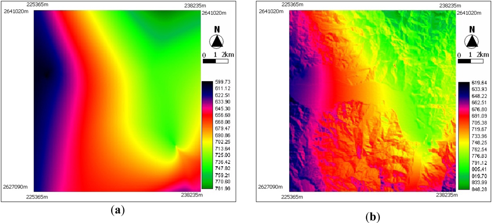
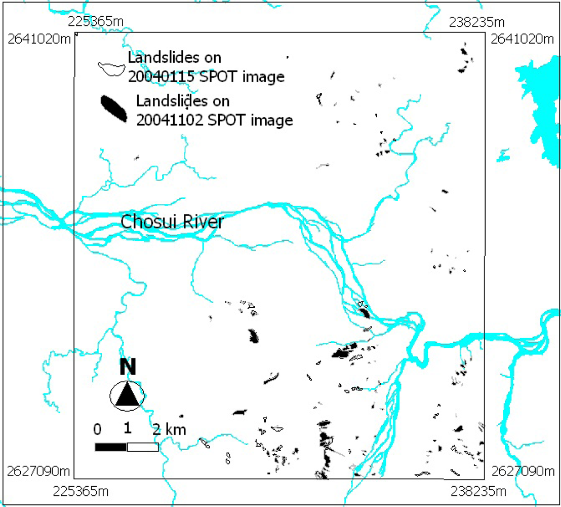
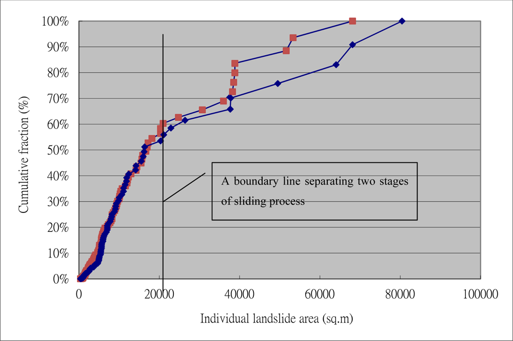
4.1. The Generation of Reference Data for Evaluation

A landslide is a highly complex subject. Understanding the occurrence of landslides is important to study their relationship with influencing factors, such as bedrock type, slope steepness, and hydrology. To interpret landslides that have already occurred, remote sensing images have been widely used. In this study, automated extraction of landslides is carried out with Satellite pour l’Observation de la Terre (SPOT) images first. The resulting landslide area is in pixels. Grouping and aggregation are then performed with morphological erosion and dilation operators. Subsequently, the landslides are mapped as a number of polygons through vectorization. All polygons smaller than 100 m² are filtered out to avoid spurious features. While there are only a few omission errors, the commission error of landslide classification based solely on spectral images can be as high as 80% [12]. In order to reduce commission error, the landslide polygon map is overlaid with an orthophoto. This manual photographic interpretation procedure ensures the accuracy of the landslide classification by removing commission errors such as roads, parking lots, and other land cover types having spectral signature similar to landslide. Two landslide maps interpreted from SPOT images were thus created. One map depicts the existing landslide areas shortly before Typhoon Mindulle and the other map represents landslides shortly after.

Two SPOT-5 scenes were selected based on image quality and cloud cover percentage. They were taken on 15 January 2004 and 2 November 2004, respectively. Characteristics of the selected images are listed in

Table 2. Characteristics of images selected in this study.

	Taken before Mindulle	Taken after Mindulle
Image ID	CSR_P0000358_SP5G1J_20040115	CSR_P0000787_SP5G1J_20041102
Receiving time	2004/01/15_02:40:31	2004/11/02_02:26:21
Viewing incidence angle	−3.088	−30.333551
Path/Row	299/300	299/301
Width/Height (Km)	121/324	149.5/391
Lines/pixels	32400(lines)/12100(pixels)	39100(lines)/14950(pixels)
Sun Elevation	39.607085	39.607085
Sun Azimuth	154.07631	153.53001
Orientation	12.9894	11.6754

. Selected images of the study area were cloud free for both dates. Images were precisely ortho-rectified with accuracy within one pixel and geo-referenced to the TWD97 Taiwan Datum coordinate system [37]. The panchromatic, multispectral, and pan-sharpened images were acquired. Multispectral images were used for automatic classification of landslides with Maximum Likelihood Method.

The slope and aspect of terrain are derived from the DEM produced by Aerial Survey Office of the Forestry Bureau. The grid size of the DEM is 40 m and its vertical accuracy is about 2.5 m [38]. For calculating rainfall vector, a local trend of slope attitude was derived using the DEM of the 40m-grid from the Aerial Survey Office of Forestry Bureau.

Orthophotos used in this study were acquired in 2002. The grid size of the orthophotos is 50 cm, which is a standard product supplied by the Aerial Survey Office of the Taiwan Forestry Bureau for civilian applications. Although aerial photographs were acquired at a different time from the SPOT images, the orthophotos were used for checking the classification results of SPOT images other than interpreting existing landslides. Commission errors occur in areas such as bare farmlands, riverbank soils, and sparsely-vegetated open spaces, and the parceling of these committed errors can be very different from the natural shapes of landslides. Therefore, it is useful to obtain a quick result from SPOT images with automatic classification, and subsequently apply a manual check to eliminate incorrect polygons with orthophotos employing conventional visual photo-interpretation methods. These steps were adopted to ensure correctness of the landslides used in subsequent analysis.

As shown in Figure 6, there were 84 existing landslides interpreted from SPOT images on 15 January 2004, the date before Mindulle and 113 landslides were observed from SPOT images on 2 November 2004, the date after Mindulle. The size of each individual landslide ranged from 100 m² to 80,000 m².

Table 3. Statistics of landslide size distribution of the study area for both before and post Typhoon Mindulle.

Class	Lower Bound (m2)	Upper Bound (m2)	By Image on 20040115		By Image on 20041102
			Slide Number	Slide Area	Slide Number	Slide Area
1	0	1,600	16	17,332	20	21,748
2	1,600	3,200	8	19,323	19	42,971
3	3,200	6,400	21	109,372	27	130,225
4	6,400	12,800	23	210,572	24	222,137
5	12,800	25,600	9	156,715	14	243,953
6	25,600	51,200	4	151,399	6	221,090
7	51,200	80,437	3	212,585	3	173,041
	Total		84	877,298	113	1,055,165

shows the statistics of different classes of landslide sizes for both before and post Typhhon Mindulle. The solid diamond in Figure 7 shows the distribution of cumulative percentage of the size of landslides existing before Mindulle. The solid square in Figure 7 is for landslides identified after Mindulle. It is shown that the cumulative area is 60% for an individual landslide with an area smaller than 25,000 m², whereas the cumulative percentage of total number of landslides under this size is 90%. In other words, most landslides were small.

In general, the size distributions of landslides for before and after Mindulle show a similar trend. The area of individual landslides is proportional to the cumulative fraction. From the curves in Figure 7, there are two linear segments. This may represent two separate landslide processes. In the first, small landslides take place and comprise the first 10 to 60% of the cumulative percentage of total landslide area. This linear trend has a high slope in this first, indicating a rapid increase of small landslides when rainfall exceeds a certain threshold. The second starts from a cumulative percentage of more than 60% where a gentle slope of the linear trend is observed in the landslides after the event as shown by solid squares in Figure 7. This indicates that large-scale landslides with areas larger than 25,000 m² are triggered after the occurrence of small landslides.

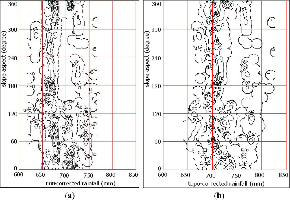
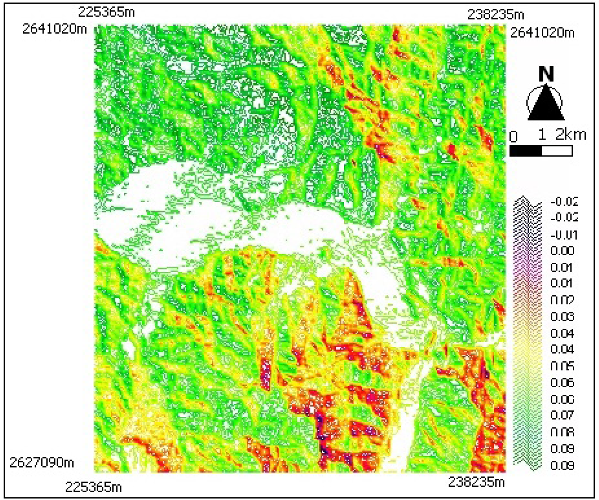
4.2. Effects of Topographic Correction with Rainfall Vectors

Wind vectors from three selected weather stations were calculated separately. Wind vectors of each grid-cell were interpolated from these stations. Since there are fewer wind stations than rain stations, it is important that the study area should be completely enclosed by the selected stations to avoid extrapolation. Similarly, rainfall vectors from all weather stations were calculated separately. Then rainfall vectors of all grid-cells were obtained by interpolation from stations. The grid size was 40 m, corresponding to the grid of DEM. Then projections of rainfall vectors onto the ground surface of each grid-cell were created.

Rainfall distribution of the study area is derived from the rain records of the ten selected weather stations with the ordinary Kriging interpolation scheme. The maximum event rainfall in the study area is 782 mm and the minimum is 600 mm. Figure 8(a) shows the result of interpolation of the average rainfalls of the 12 hours prior to the peak intensity of the Mindulle event of the ten stations. In comparison, Figure 8(b) shows rainfall distribution with topographic correction. The landform undulation is marked on the rainfall map. Maximum rainfall after correction is 848 mm and the minimum becomes 620 mm. It is noteworthy that places with minimum and maximum values do not remain at the same sites before and after correction. As described in Section 3.4, the magnitude of correction factor depends on slope attitude; the location depends on whether it is a windward slope or leeward slope. This effect is further illustrated in Figure 9, which shows the percentage of difference between the adjusted rainfall map and the original rainfall map. In general, the effect of change is 11%. In the windward aspect, an increase of 8% rainfall is estimated, whereas a maximum deduction of 2% rainfall is estimated in the leeward aspect. There are very few areas where correction factors are negative. This shows that underestimation of rainfall intensity in the windward aspect due to topographic effect was obvious.

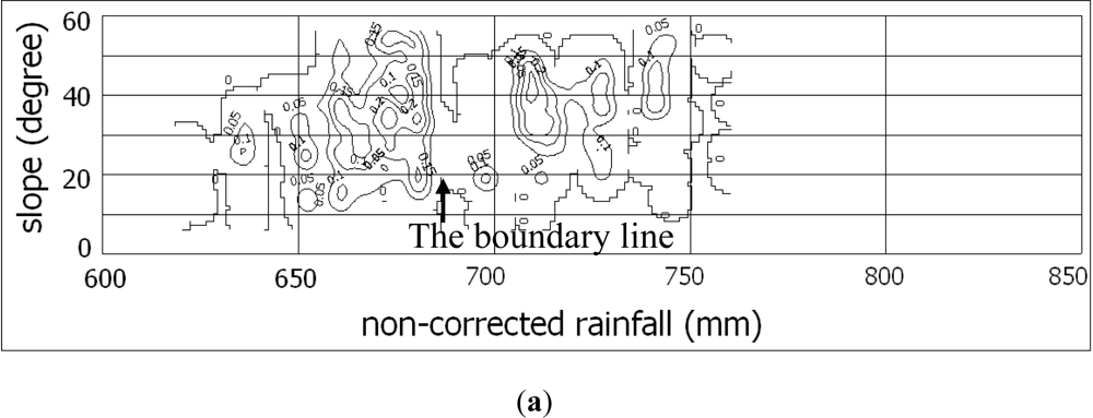
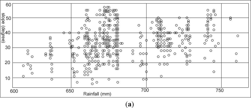
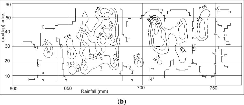
4.3. Landslide Distribution in Various Slope Aspects and Rainfall

The landslide occurrence density is shown in Figure 10. The ordinate of the vertical axis is the slope aspect and the abscissa of the horizontal axis is rainfall. Figure 10(a,b) is plotted with the landslides on SPOT images taken after Mindulle, where rainfall of Figure 10(a,b) are without and with topographic correction, respectively.

Comparing Figure 10(a) and 10(b), the general S-shaped banding of landslide density after correction is the most obvious difference. Because the prevailing windward slopes are in the aspects of 180–270 degrees of azimuth, the topographic-corrected rainfalls are raised in larger amount than those of other slope aspects. The general trend of the S-shaped banding is thus formed. If the rainfall is not corrected with topography and slope aspects, most landslides take place when rainfall is in the range of 650–680 mm with no specific influence of slope aspects. However, in the prevailing windward slopes in the aspect of 180–270 degrees, landslides take place in a very narrow band. Then the rainfall thresholds of windward slopes become more than 700 mm. In the leeward-side of 0–90 degrees of azimuth, a banded feature still exists, but it is a wider band. These features show that landslide processes in different aspects are not the same. The landslide period in windward slopes is relatively shorter, and rainfall thresholds for initiating processes are relatively higher. Both of these features are due to rainfall vectors in the opposite direction of the slope aspects.

4.4. Landslide Distribution in Various Slope Angles and Rainfall

Figure 11 shows the pattern of landslide occurrence. The vertical axis is slope angle and the horizontal axis is rainfall. Figure 11(a,b) are plotted with the landslides only on SPOT images taken after Mindulle, where rainfall of Figure 11(a,b) are without and with topographic correction, respectively.

Comparing Figure 11(a) and 11(b), it can be seen that the range of slope angles of landslides remains relatively unchanged with and without topographic correction, as expected, because slope angle of a landslide does not change even if the relationship between rainfall vector and slope attitude changes. Before rainfall is corrected, as shown in Figure 11(a), the first stage of landslides takes place in the rainfall range from 650 mm to 685 mm, and the second stage takes place in the range of 705 mm to 745 mm. However, after the rain is corrected, the concentration of the trend pattern of landslide occurrence is obvious in Figure 11(b). The first stage of landslide occurrence takes place in the range of 655 mm to 750 mm, which gives a lower threshold and wider range than the case of no topographic correction. The range in second stage is from 755 mm to 795 and is concentrated in one group.

5. Conclusions and Future Work

A rainfall-vector projection method is proposed for topographic correction. A rainfall-vector is a resultant vector combining vertical raindrop terminal velocity and a horizontal wind vector. In the case of Typhoon Mindulle of 2004, the range of the average wind vectors ranges from 2.0 to 5.0 m/s. Deviation of the angle between the rainfall vector and the vertical rainfall vector of the study area ranges from 14.45 to 34.19 degrees. The correction factor ranges from −2% to +9%.

The density of landslides derived from the scatter plot of rainfall intensity and slope/aspect is applied in this study for exploring the relation between landslide and these variables. Although we assumed non-turbulent wind and direct falling-down with no raindrop capturing processes, the rainfall intensity is more realistic with the topographic correction than without and agrees more closely with the landslide occurrence. Taiwan Typhoon and Flood Research Institute was established in 2011 and advanced observation techniques including 1D and 2D video distrometers, and various types of weather radar systems for raindrop observations and rainfall intensity observations, respectively. The datasets can be further adopted in further study of rainfall vectors of the topographic effect.

References

1. Brocca, L.; Ponziani, F.; Moramarco, T.; Melone, F.; Berni, N.; Wagner, W. Improving landslide forecasting using ASCAT-derived soil moisture data: A case study of the Torgiovannetto landslide in Central Italy. Remote Sens 2012, 4, 1232–1244. [Google Scholar]
2. Holbling, D.; Fureder, P.; Antolini, F.; Cigna, C.; Casagli, N.; Lang, S. A semi-automated object-based approach for landslide detection validated by persistent scatterer interferometry measures and landslide inventories. Remote Sens 2012, 4, 1310–1336. [Google Scholar]
3. Kasperski, J.; Delacourt, C.; Allemand, P.; Potherat, P.; Jaud, M.; Varrel, E. Application of a Terrestrial Laser Scanner (TLS) to the study of the Sechilienne Landslide (Isere, France). Remote Sens 2010, 2, 2785–2802. [Google Scholar]
4. Othman, A.A.; Gloaguen, R. River courses affected by landslides and implications for hazard assessment: A high resolution remote sensing case study in NE Iraq–W Iran. Remote Sens 2013, 5, 1024–1044. [Google Scholar]
5. Tofani, V.; Raspini, F.; Catani, F.; Casagli, N. Persistent Scatterer Interferometry (PSI) technique for landslide characterization and monitoring. Remote Sens 2013, 5, 1045–1065. [Google Scholar]
6. Yonezawa, C.; Watanabe, M.; Saito, G. Polarimetric decomposition analysis of ALOS PALSAR observation data before and after a landslide event. Remote Sens 2012, 4, 2314–2328. [Google Scholar]
7. De Lima, J. The effect of oblique rain on inclined surfaces: A nomograph for the rain-gauge correction factor. J. Hydrol 1990, 115, 407–412. [Google Scholar]
8. Helming, K. Wind Speed Effects on Rain Erosivity. Sustaining the Global Farm: Selected Papers from the 10th International Soil Conservation Organization Meeting; Stott, D.E., Mohtar, R.H., Steinhardt, G.C., Eds.; ISCO: West Lafayette, IN, USA, 1999; pp. 771–776. [Google Scholar]
9. Sharon, D. The distribution of hydrologically effective rainfall incident on sloping ground. J. Hydrol 1980, 46, 165–188. [Google Scholar]
10. Schulz, W.H. Landslide Susceptibility Estimated From Mapping Using Light Detection and Ranging (LIDAR) Imagery and Historical Landslide Records; Open-File Report 2005-1405; USGS: Seattle, WA, USA, 2005. [Google Scholar]
11. Schulz, W.H. Landslide susceptibility revealed by LIDAR imagery and historical records, Seattle, Washington. Eng. Geol 2007, 89, 67–87. [Google Scholar]
12. Liu, J.K.; Liao, Z.Y.; Lau, C.C.; Shih, T.Y. A Study on Rainfall-Induced Landslides in Alishan Area Using Airborne Lidar and Digital Photography. Proceedings of the 28th Asian Conference on Remote Sensing, Kuala Lumpur, Malaysia, 12–16 November 2007.
13. Varnes, D. J. Slope Movement Types and Processes. In Special Report 176: Landslides: Analysis and Control; Schuster, R.L., Krizek, R.J., Eds.; Transportation and Road Research Board, National Academy of Science: Washington, DC, USA, 1978; pp. 11–33. [Google Scholar]
14. Assilzadeh, H.; Levy, J.K.; Wang, X. Landslide catastrophes and disaster risk reduction: A GIS framework for landslide prevention and management. Remote Sens 2010, 2, 2259–2273. [Google Scholar]
15. Debella-Gilo, M.; Kääb, A. Measurement of surface displacement and deformation of mass movements using least squares matching of repeat high resolution satellite and aerial images. Remote Sens 2012, 4, 43–67. [Google Scholar]
16. Metternicht, G.; Hurni, L.; Gogu, R. Remote sensing of landslides: An analysis of the potential contribution to geo-spatial systems for hazard assessment in mountainous environments. Remote Sens. Environ 2005, 98, 284–303. [Google Scholar]
17. Yang, S.J.; Lin, J.J.; Cheng, C.T.; Pan, K.L.; Tsai, J.J.; Lee, C.L. Landslide Classification in Common Use in Taiwan. Proceedings of The 14th Conference On Current Researches In Geotechnical Engineering In Taiwan, Taoyuan, Taiwan, 25–6 August 2011.
18. Guzzetti, F.; Peruccacci, S.; Rossi, M.; Stark, C.P. The rainfall intensity-duration control of shallow landslides and debris flows: and update. Landslides 2008, 5, 3–17. [Google Scholar]
19. Li, M.; Shao, Q.; Renzullo, L. Estimation and spatial interpolation of rainfall intensity distribution from the effective rate of precipitation. Stoch. Environ. Res. Risk Assess 2010, 24, 117–130. [Google Scholar]
20. Salciarini, D.; Tamagnini, C.; Conversini, P.; Rapinesi, S. Spatially distributed rainfall thresholds for the initiation of shallow landslides. Nat. Hazards 2012, 61, 229–245. [Google Scholar]
21. CWB. List of Typhoons of Which Official Warning Notices Have Been Issued; Central Weather Bureau: Taiwan. Available online: http://rdc28.cwb.gov.tw/data.php (accessed on 20 July 2008).
22. Lin, J.Y. Use Radar Echoes to Analyze Three Dimensional Structure of Rainfalls. M.Sc. Thesis, Institute of Civil Engineering, National Taiwan University, Taipei, Taiwan,. 2001. [Google Scholar]
23. Wu, S.H.; Lin, P.L. Seasonal Change of Rainfall Types Observed by Disdrometers. Proceedings of Taiwan Geoscience Union Conference in 2004, Longtan Aspire Learning Complex, Taoyuan, Taiwan, 17–20 May 2004.
24. Gunn, R.; Kinzer, G.D. Terminal velocity of water droplets in stagnant air. J Meteorol 1949, 6, 243–248. [Google Scholar]
25. Lin, L.L.; Lin, H.W. The measurement of erodibility of red soils. J Chin Soil Water Conserv 1998, 30, 41–58. [Google Scholar]
26. Sheppard, B.E. Measurement of raindrop size distributions using a small Doppler radar. J Atmos. Oceanic Tech 1990, 7, 255–268. [Google Scholar]
27. Lin, P.L.; Jian, C.L.; Hsu, Y.C. The rain-drop distributions of Northern Taiwan. Proceedings of Taiwan Geoscience Union conference in 2007, Longtan Aspire Learning Complex, Taoyuan, Taiwan, 15–18 May 2007.
28. Su, C.L.; Chu, Y.H.; Chen, C.Y. Analyzing the relationship between terminal velocity of raindrops and VHF backscatter from precipitation. TAO 2004, 15, 629–645. [Google Scholar]
29. Tokay, A.; Short, D.A. Evidence from tropical raindrop spectra of the origin of rain from stratiform versus convective clouds. J. Appl. Meteorol 1996, 35, 355–371. [Google Scholar]
30. Tokay, A.; Short, D.A.; Williams, C.R.; Ecklund, W.L.; Gage, K.S. Tropical rainfall associate with convective and stratiform clouds: Intercomparison of disdrometer and profiler measurements. J. Appl. Meteorol 1999, 38, 302–320. [Google Scholar]
31. Maki, M.; Keenan, T.D.; Sasaki, Y.; Nakamura, K. Characteristics of the raindrop size distribution in tropical continental squall lines observed in Darwin, Australia. J. Appl. Meteorol 2001, 40, 1939–1412. [Google Scholar]
32. Wu, S.H. Use Disdrometer to Analyze Different Precipitation Type. M.Sc. Thesis, Institute of Atmospheric Physics, National Central University, Chungli, Taiwan,. 2006. [Google Scholar]
33. Mao, Y.Y. The Characteristics of Drop Size Distribution of Stratiform and Convective Rains in Northern Taiwan. M.Sc. Thesis, Institute of Atmospheric Physics, National Central University, Chungli, Taiwan,. 2007. [Google Scholar]
34. Arden, W.B. Medical Geography in Public Health and Tropical Medicine: Case Studies from Brazil. Ph.D. Dissertation, Louisiana State University and Agricultural and Mechanical College, Baton Rouge, LA, USA,. 2008. [Google Scholar]
35. De Smith, M.J.; Goodchild, F.M.; Longley, P.A. Geospatial Analysis; The Winchelsea Press: London, UK, 2007. [Google Scholar]
36. Longley, P.A.; Goodchild, F.M.; Maguire, D.J.; Rhind, D.W. Geographic Information Systems and Science; John Wiley & Sons: West Sussex, UK, 2005. [Google Scholar]
37. Teo, T.A.; Chen, L.C.; Chan, A.J.; Liu, C.L. The Development of Geometric Corrections System for Multi-Satellite Imagery. Proceeding of the 30th Asian Conference on Remote Sensing, Beijing, China, 18–23 October 2009.
38. Shih, H.Y.; Shih, T.Y. Error analysis of the 40m-grid DTM in the catchment of Pachang River. J. Chin. Institute Civil Hydraulic Eng 1997, 24, 46–55. [Google Scholar]
Figure 1. Wind affects rainfall intensities on various slope aspects. N demotes the number of raindrops. The parallel lines stand for rainfall vectors. A denotes the rain gauge area for collecting the rains. (a) In plain area, rainfall amount remains the same with or without horizontal wind; (b) In sloping area, rainfall amounts for leeward and windward side are affected by topographic conditions.
Remotesensing 05 02571f1
Figure 2. Study area and surrounding weather stations. Stations with diamond symbols are without wind records whereas those with circled-diamonds are with wind records. (X, Y) is the projected geodetic coordinate in Taiwan Datum TWD97. The study area is within the map sheet numbered 95201SW, with the following extent, Minimum X = 225,467 m; Maximum X= 238,283 m; Minimum Y = 2,627,010 m; Maximum Y = 2,640,911 m.
Remotesensing 05 02571f2
Figure 3. Procedure for deriving topographic-corrected rainfall.
Remotesensing 05 02571f3
Figure 4. (a) Derivation of topographic correction factor (Kt), which is the ratio of OW to OV. (b) When the azimuth of rainfall vector deviates from slope direction where the rainfall component maximize, a correction has to be applied. Delta (δ) is the deviation angle of rainfall vector from slope direction.
Remotesensing 05 02571f4
Figure 5. Landslide occurrence with respect to slope and rainfall. Each landslide is plotted as a small circle. (a) The original plot. (b) Kernel Density of (a).
Remotesensing 05 02571f5aRemotesensing 05 02571f5b
Figure 6. Spatial distribution of landslides in the study region before and post typhoon Mindulle. Location of the area is shown in Figure 2.
Remotesensing 05 02571f6
Figure 7. Distribution of cumulative percentage of landslide size as interpreted from images taken before and after Typhoon Mindulle. Solid diamonds are for those before the event whereas solid squares are for those after the event.
Remotesensing 05 02571f7
Figure 8. Rainfall distribution interpolated from surrounding rain stations (a) without topographic correction, (b) with topographic correction. Rainfall unit is in mm. Location of the area is shown in Figure 2.
Remotesensing 05 02571f8
Figure 9. Topographic correction in percentage derived from Kt.
Remotesensing 05 02571f9
Figure 10. Landslide occurrence density. (a) without topographic correction; (b) with topographic correction. Because different amounts of correction are made, the general outer shape of the concentration is thus changed.
Remotesensing 05 02571f10
Figure 11. Landslide occurrence with respect to slope and rainfall, (a) without topographic correction; (b) with topographic correction. The dark arrow shows the boundary line separating two stages of sliding processes
Remotesensing 05 02571f11aRemotesensing 05 02571f11b