Supervised Method of Landslide Inventory Using Panchromatic SPOT5 Images and Application to the Earthquake-Triggered Landslides of Pisco (Peru, 2007, Mw8.0)


Abstract
:1. Introduction
2. Data
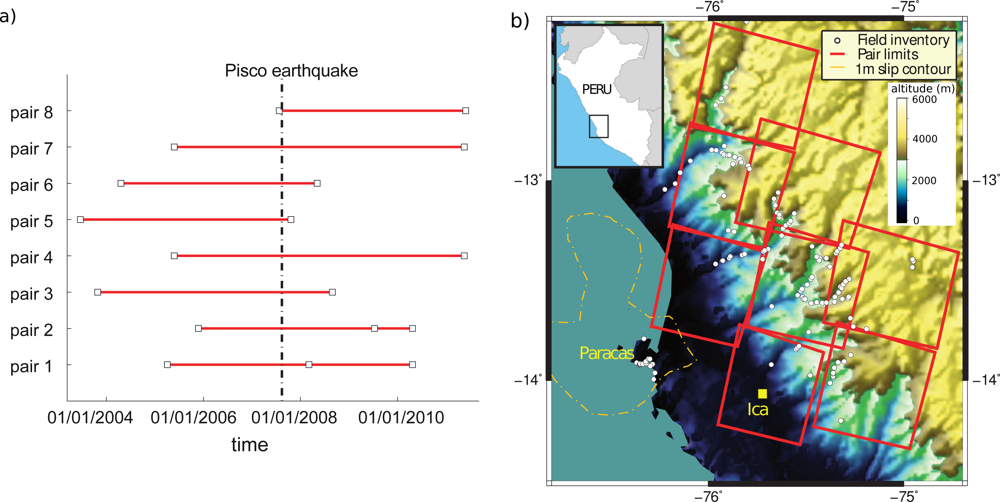
2.1. Study Area
2.2. Satellite Images
3. Methodology
3.1. Orthorectification
3.2. Clouds Detection
3.3. Change Detection
3.4. False Alarms Removal
3.4.1. Objects Definition
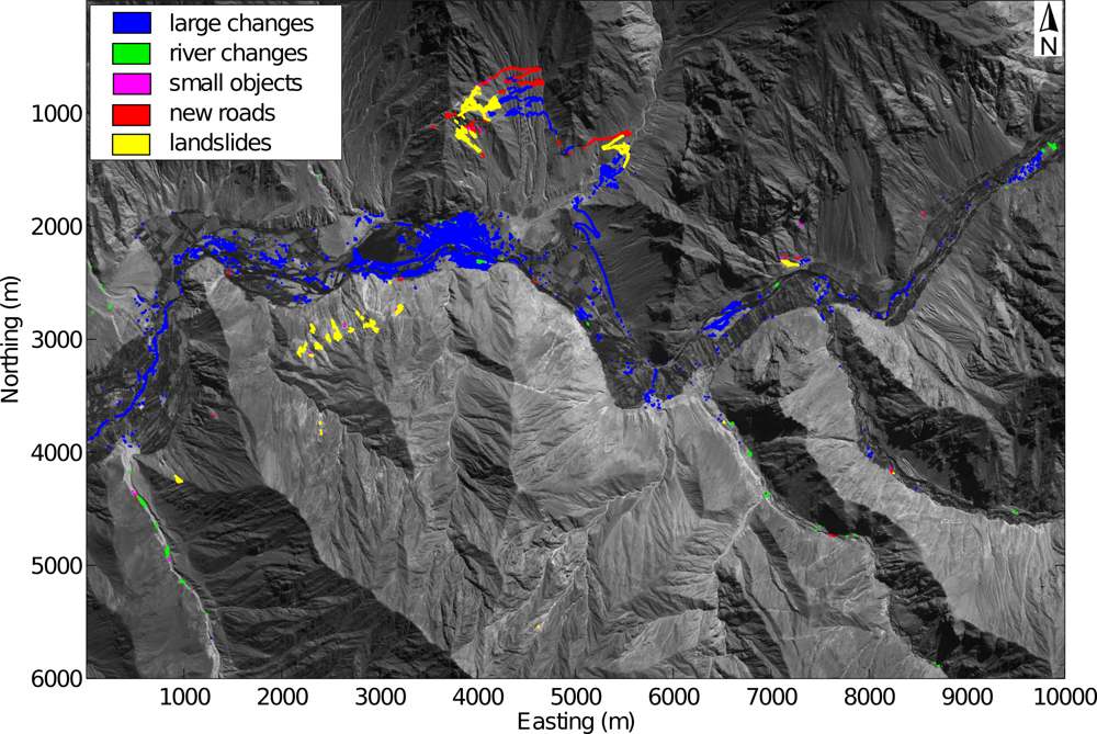
3.4.2. Change Detection at Large Scales
- We select all the objects with βo below a slope value α (Figure 3(b)). Each object has a correlation Co.
- For one of this object, we search its connected points (distant by less than w pixels) having a correlation lower or equal to Co (Figure 3(c)).
- Step 2 is iterated until no connected points display values lower than or equal to Co.
3.4.3. River Bed Variation
3.4.4. Road Detection
4. Validation
4.1. Comparison with the Field Inventory
- The field inventory is dominated by landslides of small size. Among the landslides from the field inventory covered by the images, 79% are less than 66 m3. Assuming a relation area versus volume of V = 0.146A1.33[45], we infer a size of 100 m2, or 4 pixels of a SPOT5 image. This means they are removed by our method during the step of object definition (Section 3.4).
- The field inventory is also constituted by many rockfalls (45% of the database), which are difficult to see on satellite images taken at vertical angle
- Most of the mass movements detected by the field inventory occurred on the road [36], which were already cleaned at the time of the satellite acquisitions (at least 2 months after the earthquake, see Table 1). These deposits therefore cannot be detected on the satellite images. One exception is a small landslide scar (100 m2) detected in the SPOT5 images, which furthermore matches the location of a mass movement detected on the field.
- There are uncertainties on the field inventory where no testimony exists, i.e., in arid regions the growth of vegetation is slow, and it is therefore difficult to really give a date to the observed landslides.
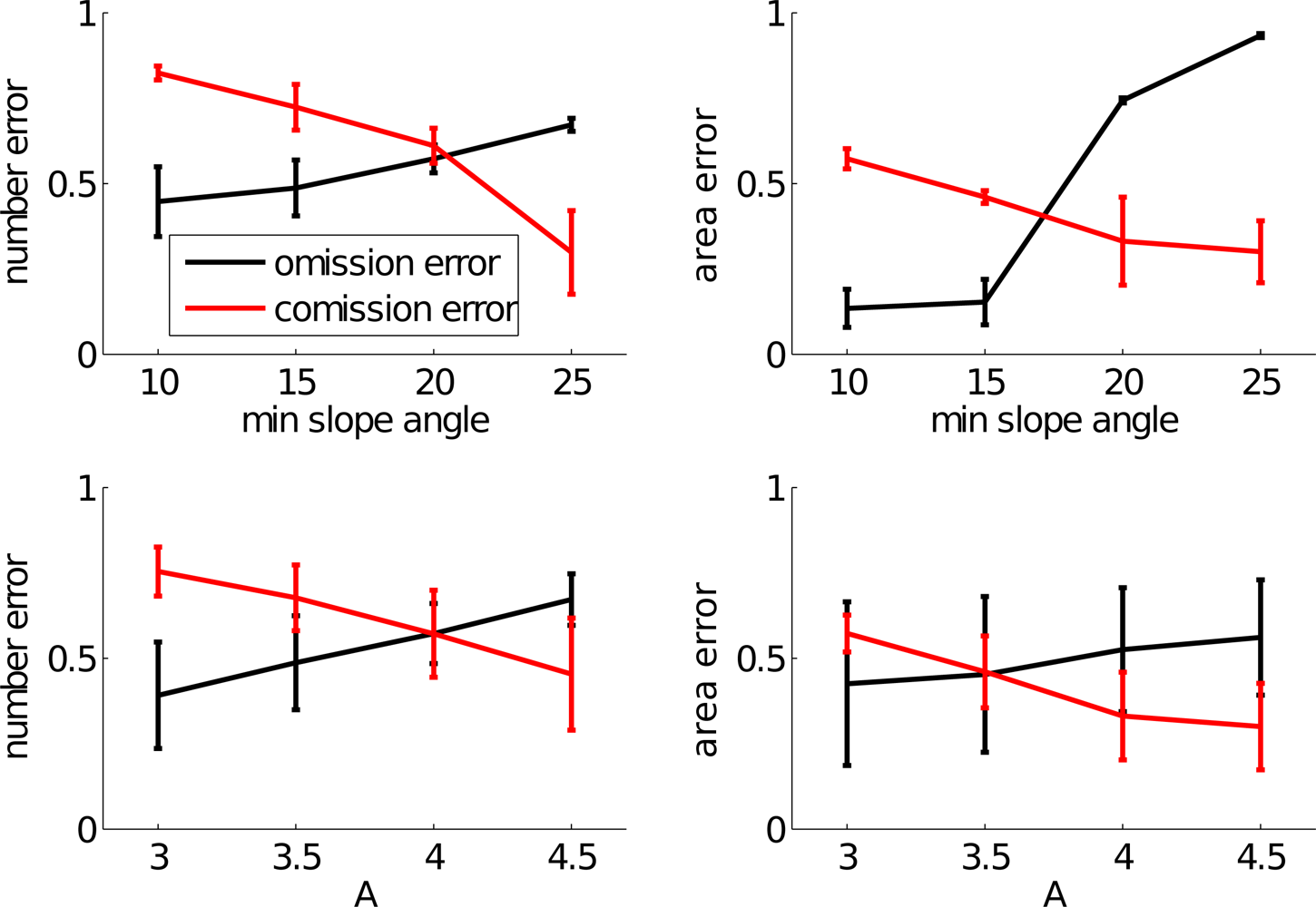
4.2. Sensitivity Analysis
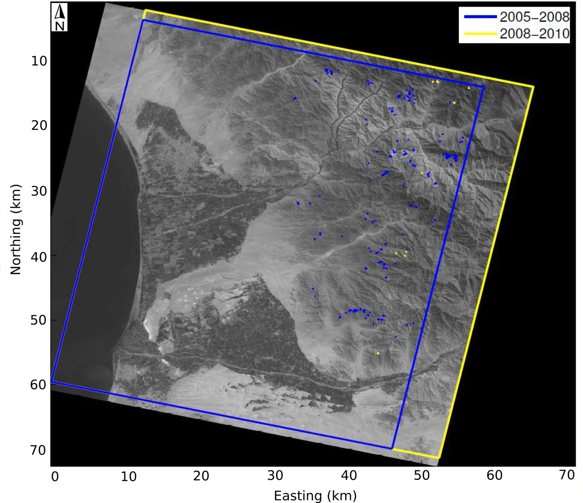
5. Application: Landslides Triggered by the Pisco Earthquake
5.1. Inventory Validation
5.2. Characteristics of the Landslide Inventory
5.3. Topographical Properties of the Landslides
6. Discussion on the Method
7. Conclusions
Acknowledgments
- Conflict of InterestThe authors declare on conflict of interest.
References
- Keefer, D.K. Landslides caused by earthquakes. Geol. Soc. Amer. Bull 1984, 95, 406–421. [Google Scholar]
- Petley, D. Global patterns of loss of life from landslides. Geology 2012, 40, 927–930. [Google Scholar]
- Keefer, D.K. Investigating landslides caused by earthquakes—A historical review. Surv. Geophys. 2002, 23, 473–510. [Google Scholar]
- Sato, H.P.; Hasegawa, H.; Fujiwara, S.; Tobita, M.; Koarai, M.; Une, H.; Iwahashi, J. Interpretation of landslide distribution triggered by the 2005 Northern Pakistan earthquake using SPOT 5 imagery. Landslides 2006, 4, 113–122. [Google Scholar]
- Gorum, T.; Fan, X.; van Westen, C.J.; Huang, R.Q.; Xu, Q.; Tang, C.; Wang, G. Distribution pattern of earthquake-induced landslides triggered by the 12 May 2008 Wenchuan earthquake. Geomorphology 2011, 133, 152–167. [Google Scholar]
- Sepulveda, S.A.; Murphy, W.; Jibson, R.W.; Petley, D.N. Seismically induced rock slope failures resulting from topographic amplification of strong ground motions: The case of Pacoima Canyon, California. Eng. Geol. 2005, 80, 336–348. [Google Scholar]
- Sidle, R.; Ochiai, H. Landslides: Processes, prediction, and land use. Water Resour. Monogr. 2006, 18, 1–312. [Google Scholar]
- Lin, G.W.; Chen, H.; Chen, Y.H.; Horng, M.J. Influence of typhoons and earthquakes on rainfall-induced landslides and suspended sediments discharge. Eng. Geol. 2008, 97, 32–41. [Google Scholar]
- Meunier, P.; Hovius, N.; Haines, J.A. Topographic site effects and the location of earthquake induced landslides. Earth Planet. Sci. Lett. 2008, 275, 221–232. [Google Scholar]
- Tang, C.; Zhu, J.; Qi, X.; Ding, J. Landslides induced by the Wenchuan earthquake and the subsequent strong rainfall event: A case study in the Beichuan area of China. Eng. Geol. 2011, 122, 22–33. [Google Scholar]
- Del Gaudio, V.; Coccia, S.; Wasowski, J.; Gallipoli, M.R.; Mucciarelli, M. Detection of directivity in seismic site response from microtremor spectral analysis. Nat. Hazards Earth Syst. Sci. 2008, 8, 751–762. [Google Scholar]
- Bozzano, F.; Lenti, L.; Martino, S.; Paciello, A.; Mugnozza, G.S. Self-excitation process due to local seismic amplification responsible for the reactivation of the Salcito landslide (Italy) on 31 October 2002. J. Geophys. Res. 2008. [Google Scholar] [CrossRef]
- Rodriguez, C.; Bommer, J.; Chandler, R. Earthquake-induced landslides: 1980–1997. Soil Dyn. Earthq. Eng. 1999, 18, 325–346. [Google Scholar]
- Galli, M.; Ardizzone, F.; Cardinali, M.; Guzzetti, F.; Reichenbach, P. Comparing landslide inventory maps. Geomorphology 2008, 94, 268–289. [Google Scholar]
- Hervas, J.; Barredo, J.I.; Rosin, P.L.; Pasuto, A.; Mantovani, F.; Silvano, S. Monitoring landslides from optical remotely sensed imagery: The case history of Tessina landslide, Italy. Geomorphology 2003, 54, 63–75. [Google Scholar]
- Barlow, J.; Franklin, S.; Martin, Y. High spatial resolution satellite imagery, DEM derivatives, and image segmentation for the detection of mass wasting processes. Photogramm. Eng. Remote Sensing 2006, 72, 687–692. [Google Scholar]
- Lee, S.; Lee, M.J. Detecting landslide location using KOMPSAT 1 and its application to landslide-susceptibility mapping at the Gangneung area, Korea. Adv. Space Res. 2006, 38, 2261–2271. [Google Scholar]
- Borghuis, A.M.; Chang, K.; Lee, H.Y. Comparison between automated and manual mapping of typhoon-triggered landslides from SPOT-5 imagery. Int. J. Remote Sens. 2007, 28, 1843–1856. [Google Scholar]
- Martha, T.R.; Kerle, N.; Jetten, V.; van Westen, C.J.; Kumar, K.V. Characterising spectral, spatial and morphometric properties of landslides for semi-automatic detection using object-oriented methods. Geomorphology 2010, 116, 24–36. [Google Scholar]
- Mondini, A.; Guzzetti, F.; Reichenbach, P.; Rossi, M.; Cardinali, M.; Ardizzone, F. Semi-automatic recognition and mapping of rainfall induced shallow landslides using optical satellite images. Remote Sens. Environ. 2011, 115, 1743–1757. [Google Scholar]
- Lu, P.; Stumpf, A.; Kerle, N.; Casagli, N. Object-oriented change detection for landslide rapid mapping. IEEE Geosci. Remote Sens. Lett. 2011, 8, 701–705. [Google Scholar]
- Martha, T.R.; Kerle, N.; van Westen, C.J.; Jetten, V.; Kumar, K.V. Segment optimization and data-driven thresholding for knowledge-based landslide detection by object-based image analysis. IEEE Trans. Geosci. Remote Sens. 2011, 49, 4928–4943. [Google Scholar]
- Stumpf, A.; Kerle, N. Object-oriented mapping of landslides using random forests. Remote Sens. Environ. 2011, 115, 2564–2577. [Google Scholar]
- Holbling, D.; Fureder, P.; Antolini, F.; Cigna, F.; Casagli, N.; Lang, S. A semi-automated object-based approach for landslide detection validated by persistent scatterer interferometry measures and landslide inventories. Remote Sens. 2012, 4, 1310–1336. [Google Scholar]
- Guzzetti, F.; Mondini, A.C.; Cardinali, M.; Fiorucci, F.; Santangelo, M.; Chang, K.T. Landslide inventory maps: New tools for an old problem. Earth-Sci. Rev. 2012, 112, 42–66. [Google Scholar]
- McKean, J.; Roering, J. Objective landslide detection and surface morphology mapping using high-resolution airborne laser altimetry. Geomorphology 2004, 57, 331–351. [Google Scholar]
- Czuchlewski, K.R.; Weissel, J.K.; Kim, Y. Polarimetric synthetic aperture radar study of the Tsaoling landslide generated by the 1999 Chi-Chi earthquake, Taiwan. J. Geophys. Res. 2003. doi: 200310.1029/2003JF000037. [Google Scholar]
- Yonezawa, C.; Watanabe, M.; Saito, G. Polarimetric decomposition analysis of ALOS PALSAR observation data before and after a landslide event. Remote Sens. 2012, 4, 2314–2328. [Google Scholar]
- Delacourt, C.; Allemand, P.; Berthier, E.; Raucoules, D.; Casson, B.; Grandjean, P.; Pambrun, C.; Varel, E. Remote-sensing techniques for analysing landslide kinematics: A review. Bull. Soc. Geol. France 2007, 178, 89–100. [Google Scholar]
- Riedel, B.; Walther, A. InSAR processing for the recognition of landslides. Adv. Geosci. 2008, 14, 189–194. [Google Scholar]
- Malamud, B.D.; Turcotte, D.L.; Guzzetti, F.; Reichenbach, P. Landslide inventories and their statistical properties. Earth Surf. Process. Landf. 2004, 29, 687–711. [Google Scholar]
- Tatard, L.; Grasso, J.R.; Helmstetter, A.; Garambois, S. Characterization and comparison of landslide triggering in different tectonic and climatic settings. J. Geophys. Res. 2010. doi: 201010.1029/2009JF001624. [Google Scholar]
- Rosin, P.L.; Hervas, J. Remote sensing image thresholding methods for determining landslide activity. Int. J. Remote Sens. 2005, 26, 1075–1092. [Google Scholar]
- Martha, T.R.; Kerle, N.; van Westen, C.J.; Jetten, V.; Vinod Kumar, K. Object-oriented analysis of multi-temporal panchromatic images for creation of historical landslide inventories. ISPRS J. Photogramm. 2012, 67, 105–119. [Google Scholar]
- Nichol, J.; Wong, M.S. Satellite remote sensing for detailed landslide inventories using change detection and image fusion. Int. J. Remote Sens. 2005, 26, 1913–1926. [Google Scholar]
- Zavala, B.; Hermanns, R.; Valderrama, P.; Costa, C.; Rosado, M. Procesos geologicos e intensidad macrosismica Inqua del sismo de Pisco del 15/08/2007, Peru. Revista de la Asociacion Geologica Argentina 2009, 65, 760–779. [Google Scholar]
- Sladen, A.; Tavera, H.; Simons, M.; Avouac, J.P.; Konca, A.O.; Perfettini, H.; Audin, L.; Fielding, E.J.; Ortega, F.; Cavagnoud, R. Source model of the 2007 Mw 8.0 Pisco, Peru earthquake: Implications for seismogenic behavior of subduction megathrusts. J. Geophys. Res. 2010. doi: 201010.1029/2009JB006429. [Google Scholar]
- Tavera; Bernal, I. The pisco (Peru) earthquake of 15 August 2007. Seismol. Res. Lett. 2008, 79, 510–515. [Google Scholar]
- Tavera, H.; Bernal, I.; Strasser, F.O.; Arango-Gaviria, M.C.; Alarcon, J.E.; Bommer, J.J. Ground motions observed during the 15 August 2007 Pisco, Peru, earthquake. Bull. Earthq. Eng. 2009, 7, 71–111. [Google Scholar]
- Berthier, E.; Vadon, H.; Baratoux, D.; Arnaud, Y.; Vincent, C.; Feigl, K.; Remy, F.; Legresy, B. Surface motion of mountain glaciers derived from satellite optical imagery. Remote Sens. Environ. 2005, 95, 14–28. [Google Scholar]
- Leprince, S.; Barbot, S.; Ayoub, F.; Avouac, J.P. Automatic and precise orthorectification, coregistration, and subpixel correlation of satellite images, application to ground deformation measurements. IEEE Trans. Geosci. Remote Sens. 2007, 45, 1529–1557. [Google Scholar]
- ASTER GDEM Validation Team. ASTER Global DEM Validation, Summary Report; Technical Report; ASTER GDEM Validation Team (METI/ERSDAC, NASA/LPDAAC, USGS/EROS); 2009. [Google Scholar]
- Singh, A. Digital change detection techniques using remotely-sensed data. Int. J. Remote Sens. 1989, 10, 989–1003. [Google Scholar]
- Im, J.; Jensen, J.R.; Tullis, J.A. Object-based change detection using correlation image analysis and image segmentation. Int. J. Remote Sens. 2008, 29, 399–423. [Google Scholar]
- Larsen, I.J.; Montgomery, D.R.; Korup, O. Landslide erosion controlled by hillslope material. Nat. Geosci. 2010, 4, 247–251. [Google Scholar]
- Zhang, Q.; Wang, J.; Peng, X.; Gong, P.; Shi, P. Urban built-up land change detection with road density and spectral information from multi-temporal Landsat TM data. Int. J. Remote Sens. 2002, 23, 3057–3078. [Google Scholar]
- Krieger, G.; Moreira, A.; Fiedler, H.; Hajnsek, I.; Werner, M.; Younis, M.; Zink, M. TanDEM-X: A satellite formation for high-resolution SAR interferometry. IEEE Trans. Geosci. Remote Sens. 2007, 45, 3317–3341. [Google Scholar]
- Dorbath, L.; Cisternas, A.; Dorbath, C. Assessment of the size of large and great historical earthquakes in Peru. Bull. Seismol. Soc. Amer. 1990, 80, 551–576. [Google Scholar]
- Stark, C.P.; Hovius, N. The characterization of landslide size distributions. Geophys. Res. Lett. 2001, 28, 1091–1094. [Google Scholar]
- Plafker, G.; Ericksen, G.E.; Concha, J.F. Geological aspects of the May 31, 1970, Peru earthquake. Bull. Seismol. Soc. Amer. 1971, 61, 543–578. [Google Scholar]
- Kampherm, T.S. Landslides Triggered by the 1946 Ancash Earthquake (Peru) and Geologic Controls on the Mechanisms of Initial Rock Slope Failure. M.Sc. Thesis, University Waterloo, Waterloo, ON, Canada. 2009. [Google Scholar]
- Parise, M.; Jibson, R.W. A seismic landslide susceptibility rating of geologic units based on analysis of characteristics of landslides triggered by the 17 January, 1994 Northridge, California earthquake. Eng. Geol. 2000, 58, 251–270. [Google Scholar]
- Dadson, S.J.; Hovius, N.; Chen, H.; Dade, W.B.; Hsieh, M.L.; Willett, S.D.; Hu, J.C.; Horng, M.J.; Chen, M.C.; Stark, C.P.; et al. Links between erosion, runoff variability and seismicity in the Taiwan orogen. Nature 2003, 426, 648–651. [Google Scholar]
- Qi, S.; Xu, Q.; Lan, H.; Zhang, B.; Liu, J. Spatial distribution analysis of landslides triggered by 2008.5.12 Wenchuan Earthquake, China. Eng. Geol. 2010, 116, 95–108. [Google Scholar]
- Kanda, R.V.; Simons, M. Practical implications of the geometrical sensitivity of elastic dislocation models for field geologic surveys. Tectonophysics 2012, 560–561, 94–104. [Google Scholar]


| Pair # | Pre-Event Date | Post-Event Date | B/H | Mean Incidence Angle |
|---|---|---|---|---|
| 1 | 2005/04/04 | 2008/03/05 | 0.0307 | 2.6 ° |
| 2008/03/05 | 2010/04/24 | 0.0076 | 2.2° | |
| 2 | 2005/11/24 | 2009/07/12 | 0.0094 | 2.3° |
| 2009/07/12 | 2010/04/24 | 0.0128 | 2.1° | |
| 3 | 2003/10/27 | 2008/08/29 | 0.0063 | 2.5° |
| 4 | 2005/05/26 | 2011/05/19 | 0.0021 | 2° |
| 5 | 2003/06/19 | 2007/10/22 | 0.0248 | 6.5° |
| 6 | 2004/04/20 | 2008/05/06 | 0.1578 | 24.3° |
| 7 | 2005/05/26 | 2011/05/19 | 0.0021 | 2° |
| 8 | 2007/07/26 | 2011/05/30 | 0.0014 | 22° |
| Name | Description | Min Value | Max Value | Section | Optimum |
|---|---|---|---|---|---|
| A | parameter related to the detection threshold | 3 | 4.5 | 3.3 | 3.5 |
| w | size (in pixel) of the correlation window | 16 | 128 | 3.4.2. | 32 |
| α | minimum slope of landslides | 10° | 25° | 3.4.2. | 15° |
| B | maximum angle between road and slope | 0° | 90° | 3.4.4. | 20° |
© 2013 by the authors; licensee MDPI, Basel, Switzerland This article is an open access article distributed under the terms and conditions of the Creative Commons Attribution license (http://creativecommons.org/licenses/by/3.0/).
Share and Cite
Lacroix, P.; Zavala, B.; Berthier, E.; Audin, L. Supervised Method of Landslide Inventory Using Panchromatic SPOT5 Images and Application to the Earthquake-Triggered Landslides of Pisco (Peru, 2007, Mw8.0). Remote Sens. 2013, 5, 2590-2616. https://doi.org/10.3390/rs5062590
Lacroix P, Zavala B, Berthier E, Audin L. Supervised Method of Landslide Inventory Using Panchromatic SPOT5 Images and Application to the Earthquake-Triggered Landslides of Pisco (Peru, 2007, Mw8.0). Remote Sensing. 2013; 5(6):2590-2616. https://doi.org/10.3390/rs5062590
Chicago/Turabian StyleLacroix, Pascal, Bilberto Zavala, Etienne Berthier, and Laurence Audin. 2013. "Supervised Method of Landslide Inventory Using Panchromatic SPOT5 Images and Application to the Earthquake-Triggered Landslides of Pisco (Peru, 2007, Mw8.0)" Remote Sensing 5, no. 6: 2590-2616. https://doi.org/10.3390/rs5062590