Investigating the Utility of Wavelet Transforms for Inverting a 3-D Radiative Transfer Model Using Hyperspectral Data to Retrieve Forest LAI

Abstract

The need for an efficient and standard technique for optimal spectral sampling of hyperspectral data during the inversion of canopy reflectance models has been the subject of many studies. The objective of this study was to investigate the utility of the discrete wavelet transform (DWT) for extracting useful features from hyperspectral data with which forest LAI can be estimated through inversion of a three dimensional radiative transfer model, the Discrete Anisotropy Radiative Transfer (DART) model. DART, coupled with the leaf optical properties model PROSPECT, was inverted with AVIRIS data using a look-up-table (LUT)-based inversion approach. We used AVIRIS data and in situ LAI measurements from two different hardwood forested sites in Wisconsin, USA. Prior to inversion, model-simulated and AVIRIS hyperspectral data were transformed into discrete wavelet coefficients using Haar wavelets. The LUT inversion was performed with three different datasets, the original reflectance bands, the full set of wavelet extracted features, and two wavelet subsets containing 99.99% and 99.0% of the cumulative energy of the original signal. The energy subset containing 99.99% of the cumulative signal energy provided better estimates of LAI (RMSE = 0.46, R² = 0.77) than the original spectral bands (RMSE = 0.60, R² = 0.47). The results indicate that the discrete wavelet transform can increase the accuracy of LAI estimates by improving the LUT-based inversion of DART (and, potentially, by implication, other terrestrial radiative transfer models) using hyperspectral data. The improvement in accuracy of LAI estimates is potentially due to different properties of wavelet analysis such as multi-scale representation, dimensionality reduction, and noise removal.

1. Introduction

Leaf area index (LAI) of vegetation canopies controls and moderates different climatic and ecological functions [1–3]. Since LAI is one of the principal factors controlling canopy reflectance [4], a large body of research has investigated the use of airborne and satellite remote sensing data for its accurate estimation [2,5–9].The majority of studies estimating LAI have employed empirically-based techniques, which are site-specific and may not be extendable to operational use, given different structural and climatic conditions [10]. In contrast, the physical approach using canopy reflectance models is based upon an understanding of the physical laws governing the transfer of solar radiation in vegetative canopies. It also works with variable measurement conditions and is better suited for many large scale applications [11,12]. Physically-based methods can also make full use of the high dimensional spectral and multiangular information provided by modern sensors [13].

Physically-based models range in complexity from simple nonlinear models to complex numerical radiative transfer models. One-dimensional (1-D) canopy radiative transfer models are among the more commonly used because of their ease of implementation and computational efficiency [14]. Such 1-D models assume that a canopy is composed of horizontal homogenous vegetation layers with infinite extent with canopy properties varying only along the vertical depth. However, heterogeneous plant stands such as forests may contain partial cover and generally exhibit horizontal variability in their structural and optical properties, and are thus poorly represented by 1-D models. The more realistic description of reflected radiation from a forest canopy can be provided by 3-D models [11,15–18]. The models are referred to as 3-D because the extinction and scattering coefficients that define photon interactions are explicit functions of the spatial coordinates [18].

The Discrete Anisotropy Radiative Transfer (DART) model is a widely used 3-D model [13,19,20]. Though it has a large set of input parameters, the number of parameters can be greatly reduced through simple approximation, making it amenable to inversion to estimate model parameters [14]. Since its first release [14], its accuracy, range of applications, and graphical user interface have been significantly improved [19]. DART uses simplifying hypotheses for simulating vegetation landscapes by dividing the scene into rectangular cells characterized by the volume and scattering properties of landscape elements. Vegetation canopies are simulated as the juxtaposition of turbid cells characterized by their leaf volume density, leaf angle distribution and optical properties. Soil surfaces are simulated with plane opaque surfaces characterized by specific optical properties. It can accurately model multiple scattering effects within canopies [20]. Radiative scattering and propagation are simulated with the exact kernel and discrete ordinate approaches. The model output predicts any specified directional sensor response. It was compared and tested within the European Commission Radiation Transfer Model Intercomparison (RAMI) experiment [21] and had an unprecedented level of agreement with other candidate models in simulating heterogeneous canopy spectra [13].

For the estimation of vegetation properties such as LAI, a model has to be inverted against measured reflectance data. Several model inversion techniques are available [16,22,23]. Traditional inversion methods like optimization techniques iteratively adjust model parameters until the modeled reflectance ‘fits’ or matches measured reflectance. These iterative optimization approaches are not feasible for complex models with slow computation time when simulating reflectance over a large number of spectral bands. Another widely used inversion method is LUT-based inversion [12,24,25]. They require construction of a database of pre-calculated reflectances as a function of key model parameters. Then, the spectrum for a particular image pixel is compared with each spectrum in the database, and the closest match to the image spectrum is found. The parameter combination that yields the closest spectrum in the database is considered to be the inversion solution [26]. The major advantage of the LUT-based approaches is that the forward modeling is divorced from the inversion procedure, and hence can be used for inversion of any complex model like DART [15,27].

Model inversion requires that for a unique determination of M parameters from N independent measurements (directional or spectral remote sensing measurements), M must be less than or equal to N[11,16,28]. Hyperspectral sensors subdivide the optical portion of the electromagnetic spectrum into a large number of narrow spectral bands. However, the inherent dimensionality of hyperspectral bands could be much lower than the total number of bands because of the noisier data and greater correlation in the measurements [29]. Such highly correlated bands artificially carry exaggerated weight and cause inversion bias [30,31]. Weiss et al.[32] reported that only a limited number of wavebands are required for canopy biophysical variable estimation. Other studies have stated that the selection of a subset of spectral bands can lead to a more stable and accurate inversion [27,31]. However, a general criterion for the selection of bands has not yet been defined. Meroni et al.[31] and Weiss et al.[32] utilized an empirical technique in which, starting from a combination of three bands, they selected bands in a stepwise manner. Such a stepwise procedure is a sub-optimal search as there is no guarantee of finding the best set of all possible combinations [31,32].

The discrete wavelet transform (DWT) has been increasingly used in recent years in the processing of hyperspectral images for a variety of purposes [33–39]. These studies have shown its importance as an effective tool for reducing the dimensionality of hyperspectral data while maintaining information content for a variety of applications. Banskota et al.[40] and Pu and Gong [41] have also demonstrated the importance of wavelet analysis for empirical estimation of LAI in different vegetation types. The utility of the wavelet transform for model inversion has also been explored and confirmed in several geophysical and seismic studies, where it is integrated in the forward modeling process and the model is inverted in wavelet domain [42,43]. Such direct integration of DWT in forward modeling is also a possibility for canopy reflectance models. The transformation and inversion can also be done in a completely offline mode (independent of forward modeling) by transforming the LUT entries and remote sensing measurements into wavelet features.

The advantages of DWT in LUT inversion are threefold. First, it transforms the correlated set of spectral features into wavelet features at different scales; the information carried at different scales is less correlated because of the orthogonal nature of transformation [39]. Second, most of the wavelet coefficients contain very low values which can be discarded by applying an appropriate threshold without losing significant information, thus affording dimensionality reduction. Third and most importantly, the wavelet transform affords a multi-resolution analysis of hyperspectral data by decomposing it into components of different spectral scales (analogous to spectral bands of different width). The sensitivity of canopy reflectance is scale dependent, as some parameters affect reflectance locally in a narrow range of spectral bands (e.g., chlorophyll), whereas, parameters like LAI, canopy cover and leaf angle affect reflectance over a much wider region of the spectrum. The multi-resolution analysis by discrete wavelet transform offers the possibility of re-distributing the effects of different parameters on canopy reflectance in a single band over wavelet coefficients at multiple scales. Hence, an individual wavelet coefficient might be sensitive to a reduced set of parameters, in contrast to the corresponding spectral measurement, potentially leading to an improved inversion of parameters.

The main objective of this study was to assess the utility of the Haar discrete wavelet transform as a feature extraction technique for accurately estimating forests LAI through LUT inversion of DART using airborne hyperspectral data (AVIRIS). We posited that the transformation of hyperspectral reflectance into wavelet features and subsequent LUT inversion in the wavelet domain might provide improved estimates of LAI. We also examined three different sets of wavelet features and their effect on inversion accuracy.

2. Background on Wavelet Transforms

A wavelet transform enables signal (data) analysis at different scales or resolutions by creating a series of shifted and scaled versions of the mother wavelet function [33,44]. The term “mother” implies that a set of basis functions {ψ_α,b(λ)} can be generated from one main function, or the mother wavelet ψ(λ) by the following equation [36]:

$${\psi }_{a,b}\left(\lambda \right)=\frac{1}{\sqrt{a}}\psi \left(\frac{\lambda -b}{a}\right)$$

(1)

where a is the scaling factor of a particular basis function, b is the translation variable along the function’s range and λ is a subset of an analyzed signal. In this study, we employ the Haar wavelet transform (DWT), which separates a discrete signal f of length n into two subsignals, each with length n/2, one being a running average and the other a running difference [45]. We refer to the running average, or trend, as the approximation vector, a. For each m = 1, 2, 3,…, n/2, the approximation coefficient is calculated as:

$$a_m=\frac{f_{2m-1}+f_{2m}}{\sqrt{2}}$$

(2)

We refer to the running difference, or fluctuation, as the detail vector, d. Each of the detail coefficients is calculated as:

$$d_m=\frac{f_{2m-1}-f_{2m}}{\sqrt{2}}$$

(3)

The subsignals of the original signal define the first level of the Haar transform, usually referred to as 1-level. As such, the approximation coefficients and detail coefficients from the first level can be referred to as a1 and d1, respectively. Computation of approximation and detail coefficients for subsequent levels is achieved by recursively applying Equations (2) and (3) to the approximation coefficients of the previous level. Since the subsignals have half the length of the previous signal, a2 and d2 will have half the length of a1, or n/4. The number of times n is divisible by two yields the possible number of decomposition levels. For example, if n = 16 = 2⁴, four levels of Haar transforms can be computed.

Mallat et al.[46] developed an efficient way to implement the Haar DWT scheme by representing the wavelet basis as a dyadic filter tree, or set of high-pass and low-pass filters. The high-pass and low-pass filters are related (their power sum is equal to one) and called quadrature mirror filters. Thus, the 1-level DWT decomposition of a signal splits it into a low pass version (approximation coefficients) and a high pass version (detail coefficients). The 2-level decomposition is performed on the low pass signal obtained from the first level of decomposition. The final results of a DWT decomposition of a spectrum are sets of wavelet coefficients, with each wavelet coefficient directly related to the amount of energy in the signal at different positions in the spectrum and at different scales.

3. Methods

3.1. Description of the Study Region

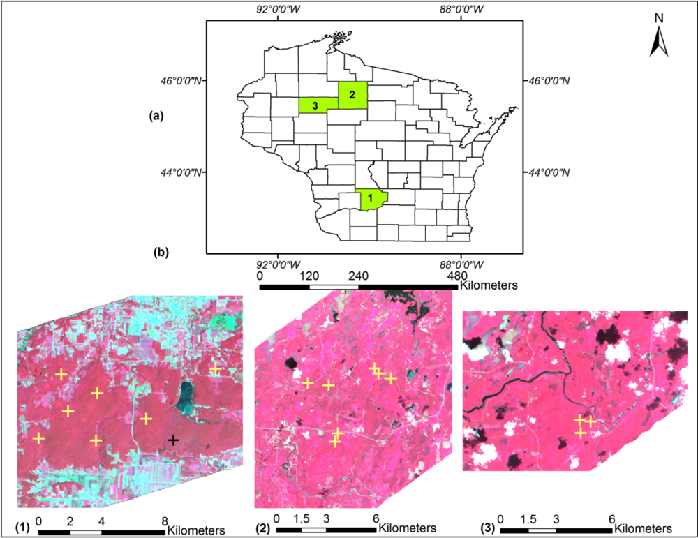
The study area comprises a range of broadleaf deciduous forest types within the state of Wisconsin, USA (Figure 1). The northernmost forest sites were located within the Northern Lakes and Forest ecoregion (90.120°W, 45.936°N to 90.318°W, 45.966°N), which is dominated by a mixed-hardwood forest originating from the large-scale clear-cut practices of the early 20th century. The overstory vegetation comprises mostly northern hardwood species dominated by sugar maple (Acer saccharum), basswood (Tilia americana), and white ash (Faxinus americana) trees), and in the lowlands by speckled alder (Alnus incanta), black ash (Fraxinus nigra) and red maple (Acer rubrum). The southern sites were located in the Baraboo Hills (89.698°W, 43.415°N to 89.845°W, 43.392°N) of the “Driftless” (unglaciated) ecoregion of Wisconsin. Most of the forests in the Baraboo Hills were cleared by the 1870s and have since recovered to forests dominated by red oak (Quercus rubra), white oak (Quercus alba), green and white ash (F. pennsylvanica and F. americana), hickories (Carya spp.), sugar maple, red maple, and basswood.

3.2. AVIRIS Image Processing

Airborne Visible/Infrared Imaging Spectrometer (AVIRIS) data used in this study (Flight ID: f080713t01 and f080714t01) were acquired in July 2008 on NASA’s ER-2 aircraft at an altitude of 20 km, yielding a pixel (i.e., spatial) resolution of approximately 17 m (16.8–17.0 m). The AVIRIS instrument produces 224 spectral bands (or wavelengths), with an approximate full-width half-maximum of 10 nm for each wavelength over the spectral range of 370 to 2,500 nm.

AVIRIS image preprocessing involved manual delineation of clouds and cloud-shadows, cross-track illumination correction, and conversion to top-of-canopy (TOC) reflectance via atmospheric correction. Redundant bands due to overlap of detectors were also removed. Cross-track illumination effects arise from a combination of flight path orientation and relative solar azimuth. We removed this effect by developing band-wise bilinear trend surfaces, ignoring all cloud/shadow-masked pixels, and trend-normalizing the images by subtracting the illumination trend surface and adding the image mean. Atmospheric correction of the cross-track illumination corrected images to TOC reflectance employed the ACORN5b™ software (Atmospheric CORrection Now; Imspec LLC, USA). Due to the low ratio of signal to noise at both spectral ends (366 nm–395 nm and 2,467 nm–2,497 nm), and in bands around the major water absorption regions (1,363 nm–1,403 nm and 1,811 nm–1,968 nm) those wavelength regions were dropped, resulting in a final total of 184 bands. The pixel spectra corresponding to the centers of the plot locations as described in the next section were extracted for the final 184 atmospherically corrected AVIRIS bands.

3.3. LAI Measurement Protocol

Optical measurements of effective LAI (L_e) were estimated from hemispherical photos collected at one meter above the forest floor using a Nikon CoolPix 5000 digital camera, leveled on a tripod with an attached Nikon FC-E8 183° lens. L_e represents the equivalent leaf area of a canopy with a random foliage distribution to produce the same light interception as the true LAI and is derived from the canopy gap fraction at selected zenith angles beneath the canopy following [47]:

$$\mathit{LAI}=\frac{L_e}{\mathrm{\Omega }}\left(1-\alpha \right)$$

(4)

where, L_e is the effective LAI, Ω is the clumping index and α is the woody-to-total leaf area ratio (α = w/L_e (1/Ω)), in which W represents the woody-surface-area-index (half the woody area per m² of ground area). In this study, we calculated LAI from L_e by correcting the effect of clumping but neglecting the effect of woods and branches in Equation (4) (i.e., LAI = L_e/Ω).

Hemispherical images were collected at 18 plots (60 m × 60 m) characterized by broadleaf decidous forest types. All measurements were made during the peak of the summer growing seasons in 2008 and 2010 during uniformly overcast skies or during dusk or dawn when the sun was hidden by the horizon. Images were collected in the JPEG format at the highest resolution (2,560 × 1,920 pixels) to maximize the detection of small canopy gaps. We followed the protocol of Zhang et al.[48] to maximize the distinction between sky and leaf/woody material. At each plot, we measured L_e at nine subplot locations: the plot center, 30 m from the plot center in each of the four cardinal directions, and the mid-point of each 30 m transect. Images were processed using DHP-TRAC software to estimate L_e and Ω, using a nine ring configuration but selecting only the first six rings for analysis to minimize the impacts of large zenith angles on the L_e retrievals and the calculation of LAI [47,49].

One broadleaf plot of our 18 total was removed from the analysis based on Cook’s Distance, which identifies influential observations on the basis of how a linear function changes when a certain observation is deleted [50]. The removed plot had the highest LAI (6.67) and unusually low reflectance throughout the near-infrared (NIR) region (maximum reflectance of 42% at NIR plateau). Cook’s test identified the plot as suspicious (partial F-statistic = 0.83, Cook’s distance = 0.97), and the reason for the discrepancy of this one plot was indeterminate, but likely due to either GPS error or disturbance to the plot between the times of data collection and imaging. The range of the LAI values for the remaining 17 plots was 2.95–5.75.

3.4. DART Scene Formulation

We used DART version 4.3.3 to simulate canopy reflectance for different parameter combinations. The DART model was run in a UNIX environment using a computer with 32 processors (eight Quad-Core AMD Opteron TM 8356 Processor) and 64 GB of physical random access memory (RAM).

DART requires users to build a computer representation of a relevant earth landscape scene such as a forest, an urban area, and water body. Ideally, the scene area should be large and should include important details about the landscape. For instance, a forest scene should be built with a large number of trees, and the resolution of the scene (cell) should be high enough to represent canopy elements such as leaves, twigs, and branches. This level of details leads to unacceptable computational time requirements for a LUT building process. Thus, a scene of reasonable size and detail needs to be determined that allows one to operate DART with an acceptable accuracy level. In this study, simulations were conducted using a simple forest representation. A repetitive forest landscape pattern made up of four trees with ellipsoid shaped crowns was chosen; previous studies have found this representations to be optimal [16,19]. The trees were described by slightly different heights (8, 9, 10, and 11 m). Both the scene size and the dimension of the tree crowns (major and minor axis) were varied to obtain scenes of different ground cover (Figure 2). The canopy was represented by foliage only, without woody branches and twigs. DART simulations with this simple forest representation is justified by the fact that the LUT building process uses mean reflectance values of the simulated images and not the 2D spatial information of these images.

3.5. Creation of LUT Database

Construction of a LUT of reflectance values for a large number of bands with a 3-D model such as DART requires an unacceptable computational time. We used an efficient strategy to populate the LUT grid with a sufficient number of DART simulations by identifying the realistic combinations of different DART parameters and their suitable ranges. The process to develop the LUT is described below.

Initially, a preliminary LUT with a wide range and coarse increments for parameters was constructed for only four narrow AVIRIS bands (550 nm, 1,139 nm, 1,692 nm, and 2,208 nm). PROSPECT [51], which is built into the DART interface, was used to calculate leaf optical properties (reflectance and transmittance). 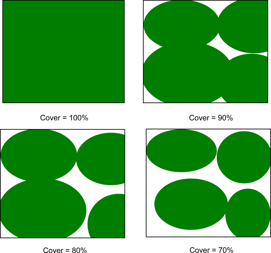PROSPECT calculates leaf hemispherical transmittance and reflectance as a function of four input parameters, leaf structural parameter (N), leaf chlorophyll a + b concentration (Cab, μg/cm²), leaf dry matter content (DM, g/cm²), and equivalent water thickness (EWT, cm). Together with the PROSPECT parameters, the parameters that were systematically varied (free parameters) were leaf area index (LAI), leaf angle distribution (LAD), soil reflectance (SL), and crown cover (CC). The range for some of the parameters (Cab, LAI, DM, and EWT) were set based upon the databases of leaf measurements spanning all common and rare tree species collected by Serbin [52] in the upper Midwest and eastern US.

The simulations in the LUT were then compared with the image reflectance to find the optimal ranges for individual parameters. The corresponding maximum and minimum reflectance values in image-extracted spectra were determined for each simulated band. The maximum and minimum values in the individual band were combined to form a maximum and minimum reflectance (max/min) spectrum. To allow for potential model/measurement uncertainties, the space was expanded by five percent in both directions. A search filter was applied to find the LUT simulations confined within the max/min space. The model inputs that led to simulations (candidate solutions) in the resulting reduced LUT were examined to infer information about optimal parameter ranges and realistic parameter combinations. Combinations of parameter values that produced similar output to image reflectance were determined as the range for the rest of model parameters for different combinations of CC, DM, and EWT. We selected the four narrow bands in the preliminary LUT as representative of the four distinct regions of the vegetation reflectance spectrum. The selection of different subsets of the candidate bands did not significantly alter our result. Once the ranges and realistic combinations were determined, a simple sensitivity analysis (SA) was performed as in Santis et al.[53] to determine the suitable incremental steps of parameter values. Based upon the results, a final LUT with finer increments for each important parameter within their narrowed ranges was built.

Table 1. Parameters, their ranges and increments for the final simulation. The final column shows the total number of values used for each parameter. The parameters are leaf area index (LAI), leaf equivalent water thickness (EWT), leaf dry matter content (DM), leaf structural parameter (N), leaf chlorophyll a + b concentration (Cab), canopy cover (CC) and leaf angle distribution (LAD). The three LADs used were planophile, plagiophile, and erectophile.

Parameters	Minimum	Maximum	Increment	Count
LAI (m2/m2)	2.75	6.75	0.25	16
EWT (cm)	0.003	0.0183	0.0017	10
DM (g/cm2)	0.001	0.0132	0.0017	7
N	1.75	2.25	0.5	2
Cab (μg/cm2)	20	60	10	5
CC (%)	70%	100%	10%	4
LAD	-	-	-	3

shows the free parameters, their minimum and maximum values, and incremental steps used for building the final LUT. The three leaf angle distributions not shown in the table were planophile, plagiophile, and erectophile LADs. A fixed value for fraction of diffuse incoming solar radiation (0.1) was used across all wavelengths. A fixed value for Lambertian soil reflectance (20%) was used because of its minimal influence on reflectance as identified by the sensitivity analysis (not shown here). This might be because of the high value for crown cover (≥70%) used in this study.

If we had considered all the parameter combinations, 134,400 (16 * 10 * 7 * 2 * 5 * 4 * 3) simulations for each AVIRIS band would have been required. After searching for realistic parameter combinations, only 5,960 simulations were needed in the infrared bands and 1,920 in the visible bands. Simulations were done separately for visible and infrared bands in order to reduce computation time, as reflectances in the two regions were sensitive to different sets of PROSPECT parameters. Canopy reflectances in the visible bands were simulated using fixed values for EWT (0.007 cm) and DM (0.007 g/cm²). Similarly, a constant value for Cab (30 μg/cm²) was used for the infrared bands. Common parameter values in both parts of the spectrum were later used to append the two tables.

3.6. Calculation of Discrete Wavelet Coefficients

When computing the DWT, two input parameters are required: the choice of mother wavelet and the level of decomposition. We chose the Haar mother wavelet as it is the simplest of all available mother wavelets, and recent investigations have illustrated its effectiveness in hyperspectral data analysis [33,36,39]. The decomposition level is determined by the type of wavelet and the original signal length. In this study, the level was chosen such that it is maximized (6 for 184 bands using the Haar wavelet). The DWT was implemented in Matlab (version 7.4, The Mathworks, Inc.) using a dyadic filter tree as described in Section 2. The hyperspectral signal in the spectral domain extracted for each pixel location was passed through a series of low pass and high pass filters. All the detail wavelet coefficients calculated at each level and approximation coefficients at final level were concatenated to produce a test dataset with 17 cases. We also calculated similar coefficients for each simulated reflectance in LUT and concatenated them with the corresponding model parameters to construct a wavelet decomposed LUT database.

3.7. LUT Inversion

LUT inversion required similarity matching between wavelet coefficients from plot spectra (measured) and the wavelet coefficients from simulated spectra (modeled). Similarity was assessed using a least root mean square error (RMSE) comparison of the simulated and measured coefficients according to Equation (5):

$$\mathit{RMSE}=\sqrt{\frac{{\sum }_{i=1}^n{\left(W_{{\mathit{measured}}_i}-W_{{\mathit{modeled}}_i}\right)}^2}{n}}$$

(5)

where, W_measured is a wavelet coefficient of measured reflectance in test dataset and W_modeled is a wavelet coefficient of modeled reflectance in the LUT, and n is the number of coefficients. The solution of the inverse problem was the set of input parameters corresponding to the reflectance in the database that provided the smallest RMSE. Because of potential insufficiency in model formulation and calibration and preprocessing errors in measured reflectance, the least RMSE solution might not necessarily provide the best estimates of LAI. According to [32], the best parameter retrieval is achieved when the number of solutions q ranges between 10 and 50. Consequently, for each of the 17 cases considered in the test dataset, q = {10, 20, 30, 40 and 50} closest matching LUT entries with the lowest RMSE were selected according to Equation (5). Out of the multiple solutions, we selected the median LAI value as a final solution.

In DWT, a large number of coefficients usually contain very low values (near-zero), and do not retain any useful information. For example, only 42 out of total 184 wavelet coefficients had 99.99% of the total energy (equivalent to variance) corresponding to original reflectance in one of the plots. The rest of the coefficients (142) had very low values (cumulatively containing only 0.01% of total energy) and might cause inversion bias. Hence, we repeated the inversion procedure but discarded the low coefficients. For each measured wavelet spectrum, the amount of retained energy by an individual coefficient was calculated as the square of its value. The wavelet coefficients were then sorted in descending order of their energies. Two sets of coefficients, which together contained 99.99% and 99.0% of the energy of original spectrum, were created. During inversion, similarity measurements between the wavelet coefficients and simulated spectra (Equation (5) were calculated using only the two subsets. For convenience, we named the wavelet set with all coefficients as ALL COEFFICIENTS and the wavelet set with 99.99% and 99.0% of energy as ENERGY SUBSET 1 and ENERGY SUBSET 2, respectively.

For comparison purposes, LUT inversion was also performed using the original spectral bands (SPECTRAL BANDS) which required assessing the similarity between plot and simulated spectra. As before, this was carried out using a least root mean square error (RMSE) comparison, in the case of the measured and modeled spectra, according to Equation (6):

$$\mathit{RMSE}=\sqrt{\frac{{\sum }_{i=1}^n{\left(R_{{\mathit{measured}}_i}-R_{{\mathit{modeled}}_i}\right)}^2}{n}}$$

(6)

where, R_measured is a measured reflectance at wavelength λ, R_modeled is a modeled reflectance at wavelength λ in the LUT, and n is the number of bands.

4. Results

LUT inversions were performed independently for all wavelet coefficients (ALL COEFFICIENTS), high energy wavelet coefficients (ENERGY SUBSET 1 and ENERGY SUBSET 2), and untransformed original spectral reflectance (SPECTRAL BANDS). All three sets of LUT were sorted from minimum to maximum according to the cost function (RMSE).

The final results are summarized in

Table 2. Results from LUT inversion. The first column shows the total number of solutions selected by least RMSEr to calculate the median LAI value. The other columns show the RMSE and R² between measured and estimated LAI by inversion using ALL COEFFICIENTS, ENERGY SUBSET 1, ENERGY SUBSET 2, and SPECTRAL BANDS respectively.

Number of Solutions (q)	All Coefficients		Energy Subset 1		Energy Subset 2		Spectral Bands
	RMSE	R2	RMSE	R2	RMSE	R2	RMSE	R2
10	0.82	0.32	0.62	0.63	0.62	0.44	0.79	0.32
20	0.69	0.43	0.50	0.75	0.60	0.49	0.65	0.46
30	0.69	0.42	0.46	0.77	0.56	0.49	0.60	0.47
40	0.71	0.34	0.49	0.70	0.58	0.41	0.62	0.41
50	0.70	0.35	0.56	0.58	0.58	0.47	0.62	0.40

. The first column of the table shows the number of solutions considered. The other columns show RMSE and R² between model inverted LAI and field measured LAI for ALL COEFFICIENTS, ENERGY SUBSET 1, ENERGY SUBSET 2, and SPECTRAL BANDS respectively.

The results show that the LAI estimated from ENERGY SUBSET 1 provided the greatest accuracy (RMSE = 0.46 and R² = 0.77), followed by the LAI estimated from ENERGY SUBSET 2 (RMSE = 0.56 and R² = 0.49). Among the different numbers of solutions, the median calculated from 30 solutions provided the best estimate of LAI, the differences were greatest for q = 10 (RMSE = 0.62) and q = 30 (RMSE = 0.46) with ENERGY SUBSET 1. The relations between the measured and model estimated LAI based on the median of 30 solutions from ENERGY SUBSET 1, and SPECTRAL BANDS are shown in Figures 3 and 4. The figures show that LAI is better estimated using ENERGY SUBSET 1 (wavelets) than using SPECTRAL BANDS.

5. Discussion

The results indicate that the discrete wavelet transform (DWT) can be a useful tool for estimating forest LAI using hyperspectral data by inverting DART. A simple wavelet decomposition of modeled and measured hyperspectral data by Haar wavelets followed by inversion using high energy wavelet coefficients provided better estimates of LAI than those provided by inversion using the original spectral reflectance.

According to Proposition 3 in Verstraete et al.[12], in order to invert a reflectance model, the number of collected uncorrelated observations must be greater than the number of the parameters in the model. Hyperspectral data provide dense observational sampling to generate sufficient variance in reflectance measurements and constrain the inversion. However, spectral measurements over narrow bands in hyperspectral data are highly correlated. Such high correlation artificially carries exaggerated weight and causes inversion bias [30–31]. The irrelevant bands not sensitive to the model parameters are also more likely to introduce noise instead of useful information and thus adversely affect the inversion accuracy [23]. Darvishzadeh et al.[13] did not find any improvement in accuracies by using spectral subsets over all wavebands in estimating grassland LAI from hyperspectral data by inversion of PROSAIL. They selected subsets (1) by stepwise linear regression, (2) based upon the importance of bands for vegetation analysis in the literature, and (3) by choosing bands considered to be well modeled by PROSAIL. On the other hand, [31] found that bands selected by a stepwise process in forward modeling performed better than the full spectrum for estimating forest LAI from DIAS airborne hyperspectral data by inverting PROSAIL. Despite its usefulness, the stepwise procedure for bands selection does not guarantee that the best set of all possible combinations will be found [31,32]. Such procedure also necessitates multiple forward runs which are not suitable for complex models like DART.

The results of this study show that the wavelet transformation of hyperspectral bands can be a useful alternative to the band selection techniques employed by previous studies. Wavelet features in this study were less correlated than the original reflectance bands owing to the orthogonal nature of the transformation. DWT also afforded dimensionality reduction, as 99.99% of the total energy was concentrated in few coefficients. Moreover, DWT provided a multi-resolution representation of the original signal in which the effects of different parameters on canopy reflectance can possibly be distributed over wavelet coefficients of different scales. A narrow band in the red edge region of the reflectance spectrum might carry signatures of different parameters including leaf pigments, LAI, etc. After wavelet decomposition, the effect of leaf pigments might be relegated to a small-scale wavelet coefficient, whereas the effect of LAI might be more pronounced in one of the large scale wavelet coefficients (as LAI generally tends to affect reflectance over a larger part of the spectrum than leaf pigments). Such decoupling of the effects over wavelet coefficients at multiple scales and consequently greater independence among parameters is a useful property for inversion. The greatest accuracy obtained by the LUT inversion using ENERGY SUBSET 1 might be attributed to one or all of these benefits offered by DWT.

The poor estimates of LAI by ALL COEFFICIENTS compared to ENERGY SUBSET 1 and ENERGY SUBSET 2 demonstrate how essential it is to select optimal wavelet features. The selection of wavelet features employed in this study was relatively straightforward as only a small fraction of coefficients retained significant information (as measured by energy). The ENERGY SUBSET 1 discarded the low coefficients and only included the top coefficients cumulatively adding up to 99.99% of total energy. By doing so, the latter represented the original reflectance with a limited number of coefficients without causing significant errors for signal representations (loss of 0.01% of total energy). One of the important properties of DWT is that the energy of the Gaussian noise component of the signal will usually be dispersed as relatively small coefficients [54]. Hence, getting rid of the low coefficients might also have helped us eliminate the noise.

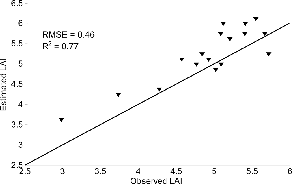
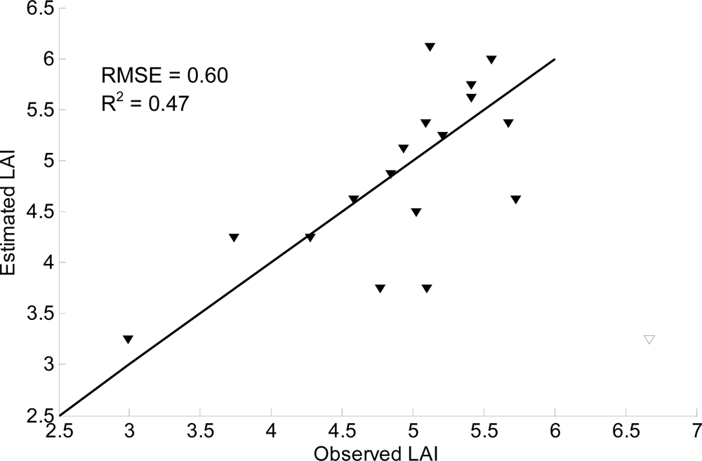
To understand the effect of different thresholds, we repeated the analysis using a new threshold of 99.0% energy. This led to a decrease in the best accuracy of LAI estimates from RMSE = 0.46 to RMSE = 0.56. With 99.0% energy, only 13 coarse-scale coefficients were retained (three approximations and others from scale level 4, 5 and 6), whereas, the 99.99% threshold level retained both coarse scale and fine scale detail coefficients from level 1 to 6. These coefficients from different levels are functions of scale and position (fine detail versus global behavior at various locations in the hyperspectral signal). The greater accuracy by ENERGY SUBSET 1, which comprises both coarse- and fine-scale coefficients, than the ENERGY SUBSET 2 implies that both the detail information and the overall trends of the hyperspectral signals are important for accurate parameter estimations by model inversion.

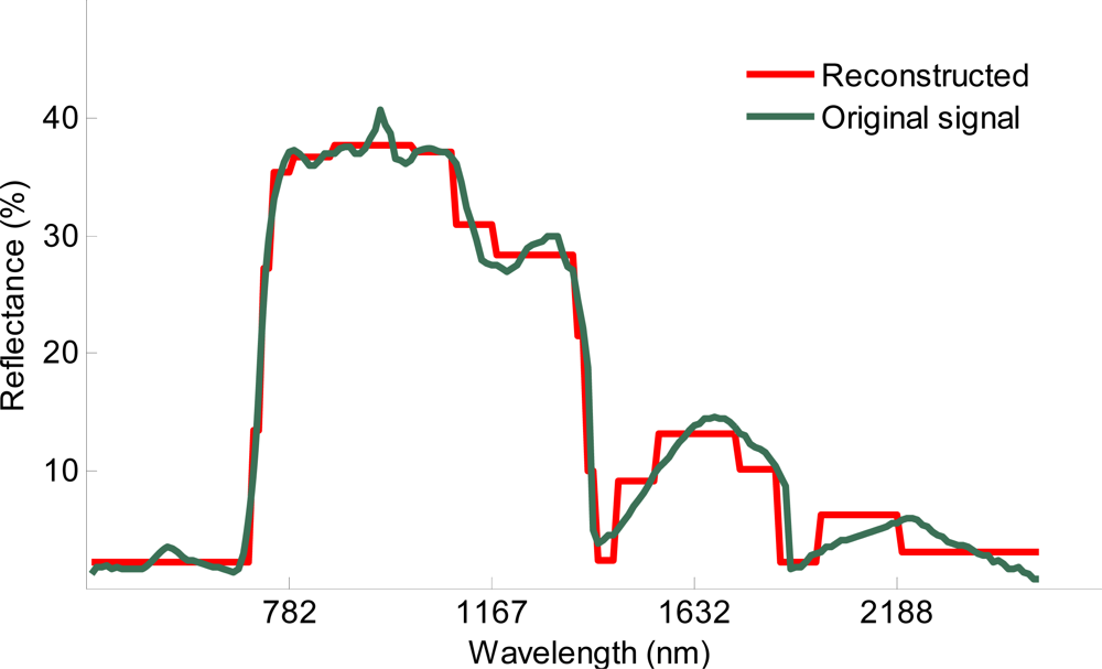
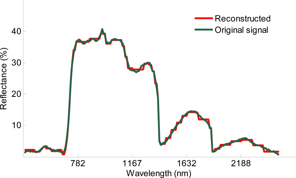
Figures 5 and 6 show the reconstruction of reflectance spectrum for one of the plots using Haar wavelet coefficients belonging to the 99.0% and 99.99% energy thresholds. The reconstructed curve was more similar to the original reflectance curve in Figure 6 than in Figure 5. Since the 99.0% threshold level selected only coarse level wavelet coefficients, the overall size and shape of the curve was preserved, but some of the important details in visible and near-infrared parts were missing. It might be possible that the best threshold level lies somewhere between 99.0% and 100% other than 99.99% used in this study, but we did not undertake a detailed analysis of the best threshold level since the main objective of this study was to demonstrate the effectiveness of DWT in DART model inversion.

The results also demonstrate that the different number of solutions estimated LAI with different accuracies. The differences were greatest between q = 10 and q = 30 with the latter providing the best estimates for all three datasets. This is consistent with the results obtained by Weiss et al. [32] as they also found 20 < q < 50 as the optimum number of solutions. RMSE increased when q increased above 30 because the distribution of solutions in terms of LAI was too wide to obtain a good estimate (median value). The highest RMSE with q = 10 indicated that the solution closely matching the test dataset might not be the best solution to estimate LAI.

We chose the Haar mother wavelet in this study, as it is the simplest of various mother wavelets, and has been found useful for hyperspectral data analysis in previous studies [33,36,39]. Pu and Gong [41] compared different families of wavelets for LAI and crown cover mapping using EO-1 Hyperion data. They found that the db3 wavelet from the Daubechies family performed best among those they analyzed. Given this, we repeated the whole analysis using the db3 wavelet to test whether the choice of a wavelet type can lead to any improvement in the accuracy of LAI estimates. We found that db3 wavelets performed slightly more poorly as compared to Haar wavelets (best RMSE for db3 = 0.49 vs. best RMSE for Haar = 0.46). The better result with db3 wavelets by Pu and Gong [41] is likely due to their use of energy features as opposed to wavelet coefficients. The Daubechies wavelet transform provides more compact redistribution of the energy of the signal than the Haar wavelet [45], so, the approximation coefficients obtained using db3 retain more energy from the original signal than those obtained using Haar. Banskota et al.[40] used a genetic algorithm to select the best subset of wavelet coefficients in regression models and found approximation coefficients less optimal than detail coefficients for explaining variation in LAI. The lower representation of the original signal by detail coefficients of db3 could be a likely explanation for different results observed in this study than that by Pu and Gong [41]. Figures 7 shows the reconstruction of reflectance spectrum for the same plot as in Figure 5 and 6 using db3 wavelet coefficients belonging to the 99.99% energy thresholds. The reconstructed reflectance curve using higher energy db3 coefficients were smoother than that by Haar coefficients but poorly represented the small variation in original signal.

The plot LAI was estimated using DHP following the protocol of Zhang et al. [48]. We acknowledge that LAI measurement uncertainty is important consideration in remote sensing research as any optical (e.g., DHP), active (e.g., Lidar) or direct measurement (e.g., litter traps, destructive harvesting) can only provide estimate of LAI [55–57]. The uncertainty in ground measured LAI is a result of the assumptions that are required for the various techniques (e.g., assumptions related to crown geometry, foliar distribution, LAD, seasonal leaf replacement or exchange, leaf optical properties, etc.) and the accuracies of measurement protocols (e.g., gap fraction, individual leaf area/mass, spatial sampling, etc.) as well as other factors that are more difficult to quantify over large areas (e.g., shoot and canopy clumping). However, given all the issues with indirect quantification of LAI, it has been well established that the properties related to clumping (at the shoot and canopy scales) are those that dominate the uncertainties [56]. Some studies have shown reasonable agreement between DHP and traditional allometric and destructive estimates (e.g., [58,59]) when properly accounting for foliage clumping. We recognize that the estimation of the degree of foliage clumping with DHP-TRAC software in this study might not provide sufficient quantification of clumping at our sites. However, given that we wanted to develop an estimate of the LAI range for which to constrain the parameter space in our DART simulations, this would not likely be a large source of error in our analysis. In other words, the bias due to imperfect characterization of canopy LAI at any one stand would not have had a significant effect on the DART simulation if the range of LAI parameterization were sufficient for the RTM runs. Figures 3 and 4 provide a comparison of DART inverted and measured LAI, which shows the minimal bias in the results, thus illustrating that we adequately parameterized DART across the range of expected LAIs that was based on our field measurements. Running simulations to quantify the uncertainty in our DART retrievals given the imperfect characterization of LAI due to any measurement uncertainty was beyond the scope of this research. In fact, to properly quantify the latter would require a detailed and careful synthesis of all uncertainties involved, preferably within a Bayesian context to sufficiently determine which assumptions/uncertainties dominate the overall error in DART retrieval of LAI (i.e., measurement error, atmospheric correction, modeling errors).

6. Conclusion

The main objective of this study was to investigate the utility of the discrete wavelet transform (DWT) for estimating forest leaf area index (LAI) via inversion of the Discrete Anisotropy Radiative Transfer (DART) model using airborne hyperspectral data (AVIRIS). The DWT transforms the hyperspectral data into wavelet features at a variety of spectral scales. The multiscale features detect and isolate variation in the reflectance continuum not detectable in the original reflectance domain such as amplitude variations over broad and narrow spectral regions. We employed the DWT on reflectance spectra obtained from hyperspectral data to improve estimation of LAI in temperate forests. The model inversion was performed with three different datasets, the original reflectance bands, the full set of wavelet extracted features, and two wavelet subsets containing 99.99% and 99.0% of the cumulative energy of the original signal. The results show that the LAI estimated from the wavelet subset with 99.99% of the cumulative energy provided the greatest accuracy. Our results suggest that the Haar discrete wavelet transform can be an effective tool for accurate DART model inversion. This study focused only on comparing multiscale DWT coefficients to the original spectral bands. The work could be extended by applying sensitivity analyses to assess the effect of variation in LAI on wavelet features at different positions and scales. Such an effort might also help identify features that are more sensitive to LAI and less to background signals caused by soil or crown cover. The theory of wavelet transforms is still developing, and more wavelet families are being introduced. The exploration of the utility of other wavelets in model inversion is well warranted since different families of wavelets are suited to different signals and applications.