Remote Sensing Based Detection of Crop Phenology for Agricultural Zones in China Using a New Threshold Method

Abstract

In recent years, the use of high temporal resolution satellite data has been emerging as an important tool to study crop phenology. Most methods to detect phenological events based on satellite data use thresholds to identify key events in the lifecycle of the crop. In this study, a new method was used to define such thresholds for identifying the start and end of the growing season (SOS/EOS) for 43 different agricultural zones in China. The method used 2000–2003 NOAA Advanced Very High Resolution Radiometer (AVHRR) satellite data with a spatial resolution of eight kilometers and a temporal resolution of 15 days. Following data pre-processing, time series for the normalized difference vegetation index (NDVI or N), slope of the NDVI curve (S), and difference (D) between the NDVI value and a base NDVI value for bare land without snow were constructed. For each zone, an optimal set of threshold values for N, D, and S was determined, based on the remote sensing data and observed SOS/EOS data for 2003 at 261 agro-meteorological stations. Results were verified by comparing the accuracy of the new proposed NDS threshold method with the results of three other methods for SOS/EOS detection with remote sensing data. The findings of all four methods were compared to in situ SOS/EOS data from 2000 to 2002 for 110 agro-meteorological stations. Results show that the developed NDS threshold method had a significantly higher accuracy compared with other methods. The method is mainly limited by the observed data and the necessity of reestablishing the thresholds periodically.

1. Introduction

Phenology is the study of periodic events in the life cycle of living species. In the case of crops, understanding the timing of periodic events in the life cycle of a crop is relevant for various activities, such as irrigation scheduling, fertilizer management, evaluating crop productivity, and analyzing seasonal ecosystem carbon dioxide (CO₂) exchanges [1]. Especially, in an increasingly food insecure world, a comprehensive understanding of global croplands is a critical need [2,3], and crop phenology is a very important element in it. Detailed information about crop phenology and in particular changes in the start and end of the crop growing seasons across China over the last 30 years are also important for the study of the impact of climate change on crops.

In recent years, the detection of phenological events using high temporal resolution satellite data (e.g., NOAA-AVHRR normalized difference vegetation index (NDVI) and Terra/Aqua-MODIS EVI) has been emerging as an important tool for ecological and climate change studies for larger areas. Many methods have been developed to detect important phenological events based on the remote sensing information. The majority of these methods consist of two key steps to (1) expand the satellite derived vegetation indices into a time series and then (2) use this time series to determine specific phenological events based on a set of rules [4].

The first step—developing the time series—involves the construction of an NDVI time series based on available data and filtering the data to reduce noise and produce a smoother time series. The primary methods for this step involve the use of various filters and functions, including the (1) Savitzky-Golay filter [4–8], which applies an iterative weighted moving filter to the NDVI time series [7]; (2) the asymmetric Gaussian function [4,7–11], which describes the NDVI time series by merging local, nonlinear fitting curves [7]; (3) the Fourier filter [9,10,12], which decomposes the NDVI time series into sine and cosine parts and filters out high frequency noise fluctuations so that a smoothed set of data can be reconstructed; (4) the logistic function, first presented by Zhang et al. [13] and enhanced to a double logistic function by Beck et al. [9] and applied in various studies [7,10]; (5) the Whittaker smoother [10,14–16], which fits a discrete series to discrete data and balances the reliability of the data and roughness of the fitted data [10]; (6) high-order splines with a roughness damping method [17], which divides the period of NDVI times series into several subintervals and defines a local Mth-order polynomial within each subinterval; and (7) the changing-weight filter method [18], in which the local maximum/minimum points in a growth cycle along an NDVI temporal profile are detected based on a mathematical morphology algorithm and a rule-based decision process, followed by a filtering of the NDVI time series with a three-point changing-weight filter.

After the time series are constructed, in the second step of most phenology detection methods, the constructed time series are analyzed to detect specific phenological events such as the start, end, and length of the growing season (SOS, EOS, and LOS) [19] based on certain rules. The most common methods for this step include threshold methods, curvature change-rate methods, harmonic analysis, moving average methods, and maximum slope and inflection point methods. Among these methods, threshold methods are common and many types exist. Examples of threshold methods include the one by Lloyd [20], who simply used an NDVI value of 0.099 as the threshold for SOS, or by Delbart et al. [21] who determined the onset of greening as the last date at which the Normalized Difference Water Index (NDWI) is lower than the minimum NDWI increased by 20% of the NDWI spring amplitude. Another threshold method was developed by Jeong et al. [19], who used the time of the maximum and minimum slope of the NDVI curve (with NDVIslope(t) = [NDVI(t + 1) − NDVI(t)]/NDVI(t)) and the corresponding NDVI value (NDVI(t)) as a threshold for determining SOS and EOS. White and Nemani [22] calculated the NDVI threshold as the value halfway between the minimum and maximum NDVI, which generally corresponds to the time of maximum NDVI increasing and decreasing, while Wu et al. [23] estimated the SOS as the time point at which the value of a fitted function first exceeds 20% of the distance between the minimum and maximum values for NDVI along the rising part of the curve. In the second category of methods, the curvature-change rate (CCR) methods, important transition dates (such as greenup, maturity, senescence, and dormancy) are defined as local minima and maxima in the curvature-change rate of logistic models designed to represent vegetation growth cycles [13]. In harmonic analysis, as described by Moody and Johnson [24], a discrete Fourier transform (DFT) is used. The analysis of the DFT harmonics provides a basis for linking the DFT results to basic vegetation types according to their characteristic phenologies. For example, SOS/EOS can be determined by analyzing the phase of the harmonics. The fourth type of method, the moving average method, was first put forward by Reed et al. [25] as the delayed moving average method to monitor the end of the growing season of crops, forest, and grass. The method was further used by Duchemin et al. [26], who applied the moving average method to monitor two key stages (budburst and senescence) in the life cycle of deciduous forests. Finally, as the last category of methods to detect phenological events in remote sensing data, maximum slope and inflection point methods can be applied. In the case of the maximum slope method, SOS and EOS are defined as the periods when vegetation growth begins to either rapidly increase (SOS) or decrease (EOS), identified based on the maximum or minimum slope of the NDVI curve [27]. In the case of the inflection point method, an algorithm is used to find valley points in the EVI/NDVI curve [1,28].

Of the various methods, threshold methods are often used as they generally keep dates within a certain reasonable range based on the threshold conditions and can thus achieve a relatively high level of accuracy. When setting thresholds, however, the characteristics of the NDVI curve are important, but these characteristics vary among crop types. Different crops have their own phenological stages during their growing seasons [29]. The use of just one threshold value for a research area, in most threshold studies, ignores the differences among crop types and physical environments. Not only crop type, but also planting patterns and climatic conditions can affect crop phenological events within a region. Therefore, it is critical to choose the “right” method for the “right” place [4] and for threshold methods to choose the “right” threshold for the “right” place. This is especially true in the case of China, with its large variety of crops growing in zones with different crop proportions and climates.

In this paper, a threshold method was introduced to study the SOS and EOS for crops in China, taking into account the varying conditions and crop proportions across the country. The method used NOAA AVHRR NDVI data and values for NDVI (N), for the slope (S) of the NDVI curve, and for the difference (D) between the NDVI value and a base value for NDVI to determine the optimal set of thresholds (for N, D, and S) for 43 agricultural zones, with different crop proportions and climate conditions. The method further used the combination of three threshold values (for N, S, and D) for each zone, to increase the percentage of accepted pixels in each zone for which an appropriate threshold can be defined. Results were verified using field observation data and the method’s accuracy was compared to those of three other phenology detection methods.

2. Materials and Methods

2.1. Materials

NOAA-AVHRR NDVI data for 2000–2003 with a spatial resolution of 8 km and a temporal resolution of 15 days was obtained from the Global Inventory Monitoring and Modeling Studies (GIMMS) group. Data corrections (e.g., for aerosols, clouds, volcanic ash, and sensor degradation) had already been performed to improve data quality [30]. The datasets were developed by the maximum value composite (MVC) technique, which produces a composite image over a fixed period of time by retaining for each pixel the maximum NDVI value from daily images [23]. For each month, two composite images were available and the early composite was assigned to the first day of the month, while the late composite was assigned to the 16th day of the month [22]. For this study, AVHRR NDVI data was chosen over the higher quality MODIS data, to be able to use the method to study changes in crop phenology in China over the last 30 years. MODIS data is not available for that entire time frame.

Data about percentages of cropland (1:100,000) across China [31] was used to derive cropland density at a resolution of 8 km (Figure 1).

In situ observation data of the SOS and EOS of major crops at 261 agro-meteorological stations was obtained from China Meteorological Administration (CMA). The 2003 data from these stations were used to determine phenology thresholds for the various agricultural zones, while 2000–2002 data from 110 stations were used to verify results. The stations for which 2003 data was used are all located in an area with a percentage of cropland above 50% (see Figure 1), as identified by the percentage of cropland for the pixel corresponding to the station location. The 110 sites used to provide 2000–2002 data for verification were selected for having a planting pattern consistent with that of the agricultural zone in which they are situated. For the in situ data, the SOS for spring wheat, corn, and soybean was defined as the crop’s seeding stage. For winter wheat, the SOS was defined as the time of returning-green, while for rice the time of transplanting was used as the SOS. For all crops the mature period of the crop was defined as EOS. In the case of double cropping and triple cropping, only the observed date of the SOS of the first growing season and the EOS of the last growing season were used.

Selection of the various agricultural zones for China, based on crop proportions and climate conditions, was based on Meng et al. [32], who divided China into 43 zones based on temperature, precipitation, solar radiation, landform, and planting pattern indices (see Figure 2).

To identify snow coverage, MOD10A2 data was used. This data was provided by the National Snow and Ice Data Center (NSIDC).

2.2. Methods

To determine and verify thresholds for SOS/EOS for the different agricultural zones in China, the methodology for this study included three distinct phases as presented in the flowchart in Figure 3. First the data was preprocessed to get high-quality NDVI time series for all pixels with a percentage of cropland above 50%. Next, statistical analysis of remote sensing data compared with field observations and an algorithm were used to determine threshold values for SOS and EOS. Finally, results were verified with in situ data and compared to other threshold methods to analyze the method’s accuracy. All of the steps will be discussed in detail below.

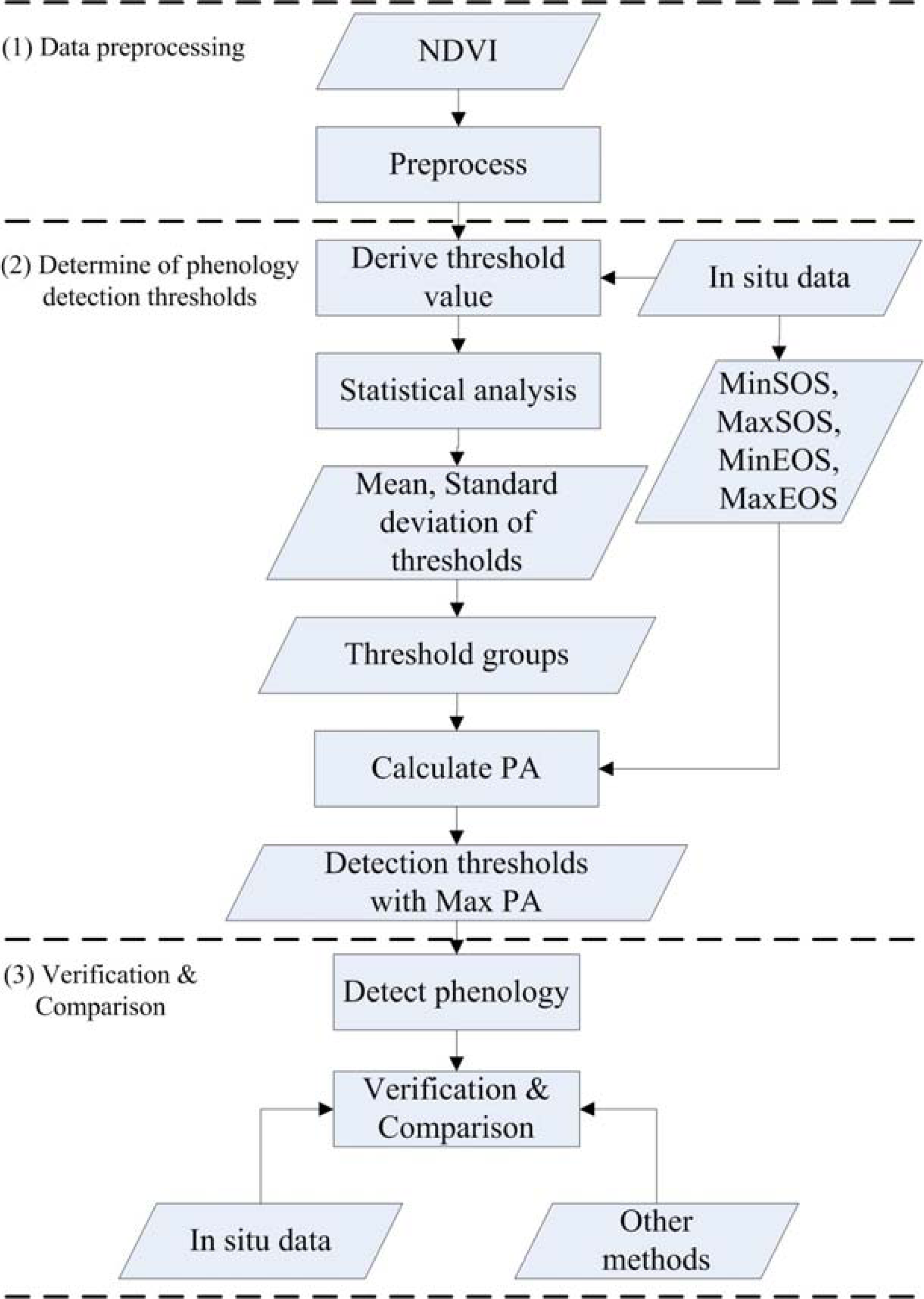
2.2.1. Data Preprocessing

Although it is generally acknowledged that composite NDVI images can greatly reduce cloud and other atmospheric noise while retaining dynamic vegetation information, residual atmospherically related noise, as well as some noise due to other factors (e.g., surface anisotropy), remain in the NDVI datasets [25]. To further remove noise and reconstruct a high-quality NDVI time-series dataset, a developed Savitzky-Golay filter was applied [6], followed by a linear interpolation of daily NDVI values for each pixel [22].

Because the study focuses on crop phenology, only pixels with a crop density greater than 50% were defined as cropland and included in the study. Pixels with or less than 50% cropland were excluded to eliminate the effect from bare land and natural vegetation as much as possible.

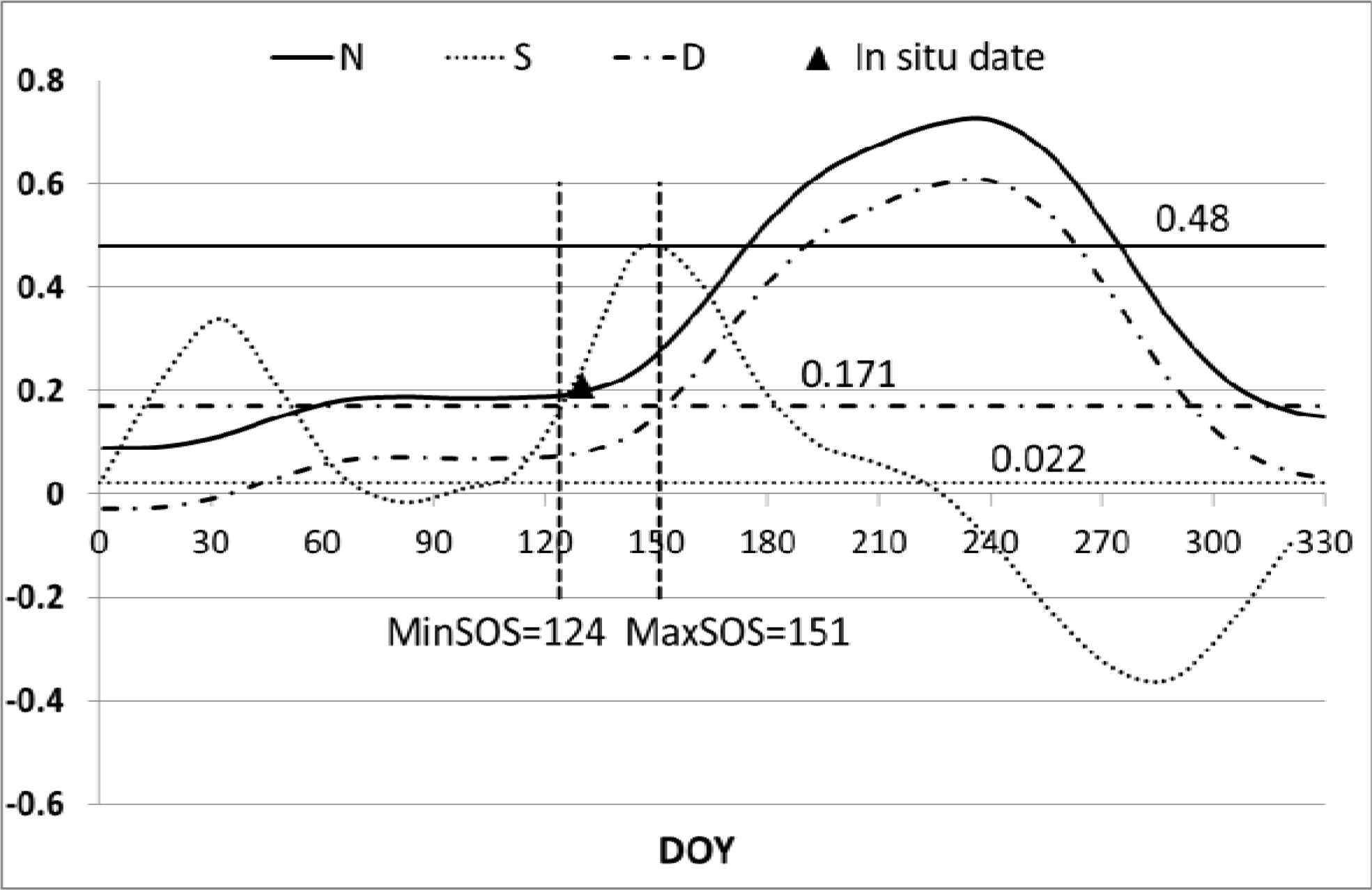
2.2.2. Determining Thresholds for Phenology Detection

The proposed method is based on the principles of the threshold method, in which the SOS and EOS are assumed to occur when the NDVI exceeds a certain value [33]. Unlike other threshold methods, the method in this study uses a combination of three threshold values for (1) NDVI, (2) the slope of the NDVI curve, and (3) the difference between the NDVI value and a base value.

First, the NDVI time series is used to determine time-series for the other two possible threshold values: slope and difference. The slope (S) of the NDVI curve describes the growing rate of the crops (Equation (1)) [34],

$$S(i)=\frac{\mathit{NDVI}(i+1)-\mathit{NDVI}(i)}{\mathit{NDVI}(i)}$$

(1)

where S(i) is the slope value of date i, NDVI(i) is the NDVI value of date i, and NDVI(i + 1) is the NDVI value of date i + 1.

Difference (D) is defined as the difference between the NDVI value on a given date and a base value for the pixel representing the NDVI of bare soil. This base value is calculated as the average of the three lowest NDVI values in a year. For cropland areas with snow cover during the winter, the three lowest NDVI values are used for when the ground is not covered by snow, as identified by the MOD10A2 data from the National Snow and Ice Data Center (NSIDC). Formula 2 shows the calculation of difference (D) between NDVI and the base value:

$$D(i)=\mathit{NDVI}(i)-\frac{\mathit{NDVI}(l)+\mathit{NDVI}(m)+\mathit{NDVI}(n)}{3}$$

(2)

where NDVI(l), NDVI(m), and NDVI(n) are the lowest three NDVI values in a year.

Following the construction of the time series for S and D for each pixel with a crop land area above 50%, field observed dates for SOS/EOS for 2003 at 261 agro-meteorological stations across China are used to identify the corresponding NDVI (N), Slope (S), and Difference values (D) for the time of SOS and EOS at each station, as shown in Figure 4. These are the N, S, and D values of the pixel associated with each station. These N, S, and D values for the various stations in a zone are used to calculate the mean and standard deviation (Stdev) for N, S, and D for each zone.

Next, also for each zone, the range of acceptable values for SOS and EOS is determined based on the observed dates of SOS and EOS for the stations in a zone. This acceptable range is from a minimum SOS (MinSOS) to a maximum SOS (MaxSOS) or from a minimum EOS (MinEOS) to a maximum EOS (MaxEOS). If the difference between the first and last observed SOS within a zone is less than or equal to 30 days, the SOS range for that zone is defined by those two values. If the difference between those two observed dates is above 30 days, the mean SOS of the two values is calculated and the range is identified as the [mean_SOS − 15, mean_SOS + 15]. Similarly, in the case of EOS, the acceptable range is defined as the dates between the first and the last observed value for EOS (at any of the stations in a zone) if the difference is less than or equal to 30 days, or as a range of [mean_EOS − 15, mean_EOS + 15] if the difference is larger than 30 days. These ranges will be used to identify which findings of SOS and EOS will be deemed “acceptable” as described below.

In a few zones, no, or just one or two, stations are present. In those cases, the zones are combined with adjacent zones with similar planting patterns to calculate the mean and standard deviation for N, S, and D, as well as the [MinSOS, MaxSOS] and [MinEOS, MaxEOS] ranges for the combined zone. Specifically, considering the spatial relationship and crop proportions, zones have been combined as follows: zones 1–1, 1–2, 1–4, and 5-1; zones 4-2 and 1–11; zones 2–3 and 2–4; zones 4–5 and 4–8; zones 4-3 and 4–14; zones 3–11 and 3–13; and zones 1–3, 3–3, and 3–9.

With the mean and Stdev for N, S, and D values determined for each zone (based on the N, S, and D values corresponding with the SOS or EOS at each station in a zone), the possible range and values for N, D, and S as threshold values for SOS/EOS detection are defined as: Mean − Stdev to Mean + Stdev, with a step increase of 0.2 × Stdev. If for example the mean N for an agricultural zone is 2 and the Stdev 1, the possible range is N = 1; 1.2; 1.4; 1.6; 1.8; 2.0; 2.2; 2.4; 2.6; 2.8; and 3.0, for a total of 11 values for that zone. Similarly, possible values for S and D will also form 11 options in a range. This way, for each zone, (11 × 11 × 11=) 1,331 different combinations or groups of N, D, and S are determined.

Next, these 1,331 different groups for each agricultural zone are tested using the algorithm shown in Figure 5. Separate analyses are done for SOS and for EOS. For each group of values, first N, then D, and then S is used to determine the SOS (or EOS) for each pixel (with above 50% cropland) within the zone. This is done by identifying the SOS (or EOS) that corresponds with the particular N (or S or D) value being tested. The algorithm tests the values in the order of N→D→S and compares the resulting SOS or EOS date for the pixel with the acceptable range ([MinSOS, MaxSOS], [MinEOS, MaxEOS]) in the zone (or as determined by combining zones). If an SOS date for a pixel based on the N threshold falls outside the range of acceptable SOS values for that zone, the result is not accepted and the algorithm moves on to use the D threshold to calculate the SOS. If the result of the D value is not accepted, the S value is used. If the result is still not accepted, the pixel is marked as denied. For each zone, all groups of thresholds are analyzed and for each group the total percentage of accepted pixels (PA) is calculated. The PA is determined as the total number of pixels (with above 50% cropland) divided by the total number of accepted pixels in the zone. The group of threshold values with the highest PA is then considered the appropriate threshold for the zone.

2.2.3. Comparison and Verification

To assess its accuracy, the method in this study (the NDS threshold method) was compared with three other methods to detect SOS/EOS events based on remote sensing data. The first method used to compare results is a curvature-change rate method (CCR) described by Zhang et al. [13]. The second is a maximum slope (MSL) method used by Yu et al. [27]. In this method the date corresponding to a maximum rate in the rise and decline of the NDVI curve is defined as SOS and EOS, respectively. Both methods were chosen for their common and global application. The third method, the threshold method (THR) by White and Nemani [22], is also very common and used widely. In this method, for each pixel the threshold is defined as the value halfway between the minimum and maximum of the annual NDVI curve.

Verification is a key element of remote sensing-based studies of phenology that cover large areas [35]. In this study, results were also verified by comparing the findings of the proposed NDS method and the other three methods with observed SOS/EOS for 2000–2002 at 110 agro-meteorological stations.

The 110 agro-meteorological stations selected for verification are again located in areas where the percentage of cropland exceeds 50% of the total area. The stations also have the same crop proportions as the corresponding zone. For each year and method, a scatterplot, analysis of linear regression (y = ax + b), the root mean square error (RMSE), bias, dispersion, and correlation coefficient between detection value and in situ data are presented. Formulations of RMSE, bias and dispersion are as follows [36]:

$$\mathit{RMSE}=\sqrt{\frac{\sum _i^N{\left(x_i-y_i\right)}^2}{N}}$$

(3)

$$\mathit{Bias}=\frac{\sum _i^N\left(x_i-y_i\right)}{N}$$

(4)

$$\mathit{Dispersion}=\sqrt{\frac{1}{N-1}\sum _i^N{\left(x_i-y_i-\mathit{Bias}\right)}^2}$$

(5)

where x_i is the value obtained by remote sensing, y_i is the in situ data in a given year, and N is the total number of verification stations.

In addition, to quantitatively describe by how much accuracy can be improved by using method A compared to method B, the following formula is used to describe the relative accuracy of method A:

$${\mathit{RIA}}_{\text{A},\text{B}}=\frac{{\mathit{RMSE}}_{\text{B}}-{\mathit{RMSE}}_{\text{A}}}{{\mathit{RMSE}}_{\text{B}}}\times 100\%$$

(6)

Where RIA_A,B is the relative accuracy of method A compared to method B. RMSE_A and RMSE_B are the RMSE of the results of methods A and B, respectively.

3. Results and Discussion

3.1. Phenology Detection Thresholds for the Agricultural Zones

Table 1. Groups of detection thresholds for SOS, MinSOS (in Day of Year (DOY)), MaxSOS (DOY), and percentage of accepted pixels (PA) for each zone. N = NDVI; D = Difference; S = Slope.

Zone	N	D	S	Min SOS	Max SOS	PA	Zone	N	D	S	Min SOS	Max SOS	PA
1-1	0.183	0.183	0.02	114	136	95%	3-8	0.43	0.124	0.006	96	126	93%
1-2	0.183	0.031	0.02	114	136	91%	3-9	0.222	0.081	0.007	85	110	93%
1-3	0.284	0.016	0.005	85	110	88%	3-10	0.343	0.009	0.003	92	122	25%
1-4	0.198	0.031	0.02	114	136	89%	3-11	0.413	0.152	0.003	117	139	66%
1-5	0.47	0.191	0.007	138	163	87%	3-12	0.469	0.067	0.004	88	118	72%
1-6	0.144	0.102	0.007	103	133	95%	3-13	0.512	0.288	0.008	117	139	73%
1-7	0.158	0.005	0.005	58	88	50%	4-1	0.108	0.053	0.003	93	123	76%
1-8	0.117	0.122	0.011	84	114	84%	4-2	0.238	0.003	0.008	37	55	96%
1-9	0.12	0.138	0.007	93	123	80%	4-3	0.46	0.059	0.015	94	124	28%
1-10	0.233	0.024	0.007	49	67	91%	4-4	0.316	0.008	0.01	37	67	92%
1-11	0.36	0.013	0.009	37	55	98%	4-5	0.432	0.098	0.007	72	102	57%
2-1	0.135	0.232	0.01	121	151	80%	4-6	0.416	0.034	0.002	77	107	80%
2-2	0.48	0.171	0.022	124	151	85%	4-7	0.222	0.259	0.003	120	148	92%
2-3	0.367	0.013	0.011	45	61	89%	4-8	0.248	0.061	0.001	72	102	25%
2-4	0.383	0.009	0.004	45	61	38%	4-9	0.144	0.117	0.007	103	133	94%
3-1	0.461	0.134	0.015	109	139	65%	4-10	0.162	0.056	0.004	100	130	89%
3-2	0.416	0.097	0.005	90	120	91%	4-11	0.512	0.278	0.009	123	137	85%
3-3	0.429	0.048	0.003	85	110	86%	4-12	0.273	0.272	0.01	126	156	69%
3-4	0.54	0.167	0.009	123	153	42%	4-13	0.159	0.01	0.004	86	116	82%
3-5	0.113	0.001	0.008	54	84	97%	4-14	0.488	0.116	0.003	94	124	27%
3-6	0.297	0.22	0.001	119	149	97%	5-1	0.3	0.031	0.024	114	136	58%
3-7	0.484	0.172	0.007	111	146	86%	Total						77%

presents an overview of the group of values for N, D, and S for each zone that were determined to be the optimum set of thresholds for the detection of SOS in that zone. The table further shows the acceptable range for SOS (MinSOS and MaxSOS) in the zone, as well as the percentage of accepted pixels (PA).

Table 2. Groups of detection thresholds for EOS, MinEOS (DOY), MaxEOS (DOY), and percentage of accepted pixels (PA) for each zone. N = NDVI; D = difference; S = Slope.

Zone	N	D	S	Min EOS	Max EOS	PA	Zone	N	D	S	Min EOS	Max EOS	PA
1-1	0.464	0.18	−0.02	234	253	92%	3-8	0.592	0.208	−0.005	293	303	66%
1-2	0.464	0.113	−0.02	234	253	45%	3-9	0.377	0.183	−0.001	295	325	86%
1-3	0.222	0.126	−0.006	295	325	68%	3-10	0.535	0.252	−0.004	237	267	64%
1-4	0.464	0.113	−0.02	234	253	58%	3-11	0.488	0.213	−0.004	222	252	88%
1-5	0.297	0.156	−0.026	271	281	97%	3-12	0.507	0.136	−0.016	277	307	88%
1-6	0.411	0.168	−0.003	218	240	93%	3-13	0.55	0.332	−0.006	222	252	78%
1-7	0.326	0.143	−0.002	264	280	75%	4-1	0.501	0.16	−0.015	240	269	95%
1-8	0.486	0.262	−0.004	251	281	77%	4-2	0.441	0.137	−0.016	263	281	98%
1-9	0.352	0.155	−0.037	247	267	76%	4-3	0.373	0.182	−0.008	272	296	86%
1-10	0.533	0.198	−0.006	252	267	73%	4-4	0.419	0.179	−0.023	255	285	97%
1-11	0.414	0.175	−0.005	263	281	93%	4-5	0.426	0.191	−0.013	251	281	66%
2-1	0.462	0.192	−0.006	251	271	97%	4-6	0.571	0.197	−0.004	267	297	76%
2-2	0.456	0.221	−0.021	259	281	99%	4-7	0.356	0.245	−0.03	265	273	100%
2-3	0.343	0.185	−0.02	255	285	95%	4-8	0.483	0.219	−0.004	251	281	77%
2-4	0.483	0.236	−0.011	255	285	74%	4-9	0.411	0.141	−0.013	251	271	94%
3-1	0.386	0.201	−0.003	277	306	93%	4-10	0.305	0.152	−0.006	259	289	99%
3-2	0.365	0.188	−0.002	280	310	82%	4-11	0.446	0.351	−0.006	232	240	83%
3-3	0.415	0.14	−0.002	295	325	68%	4-12	0.355	0.195	−0.027	255	281	100%
3-4	0.447	0.146	−0.007	263	293	88%	4-13	0.223	0.048	−0.018	261	279	91%
3-5	0.354	0.137	−0.016	261	291	100%	4-14	0.415	0.115	−0.012	272	296	87%
3-6	0.426	0.191	−0.004	252	279	48%	5-1	0.464	0.18	−0.02	234	253	63%
3-7	0.471	0.136	−0.006	283	299	79%	Total						88%

shows similar results for EOS.

Both for SOS and EOS, the PA exceeds 80% in most of the zones. The PA of the whole study area is also about 80%. This means that denied pixels form only a small fraction of the total number of pixels. The tables also show rather large variations in detection thresholds among zones, with the exception of some zones that are more similar and adjacent to each other. This variation in threshold values among zones reflects the wide distribution of cropland, diverse climatic conditions, and variety of crop proportions in China, as a result of which, the characteristics of the NDVI curves vary among zones. The detection thresholds determined for each zone follow those characteristics.

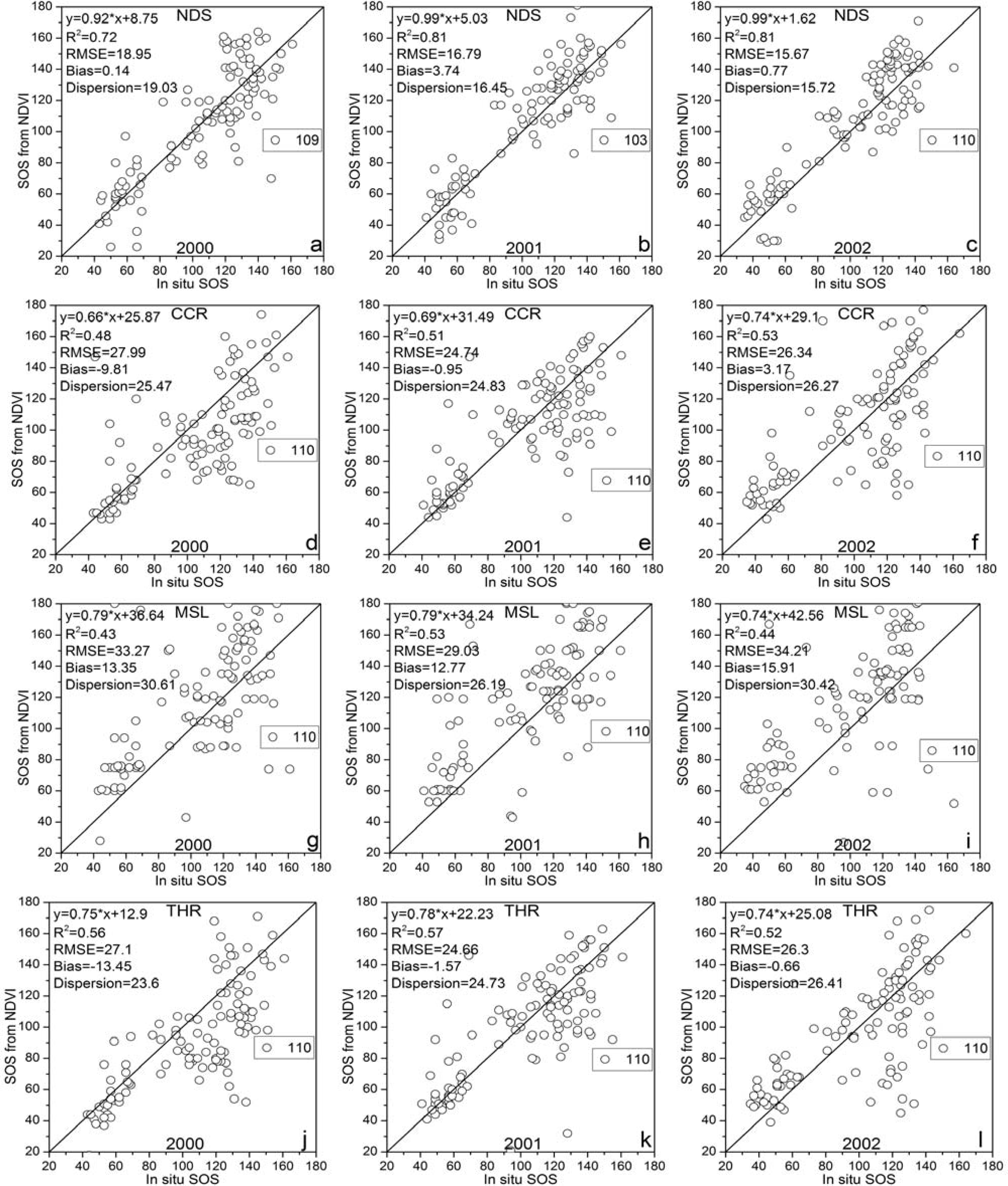
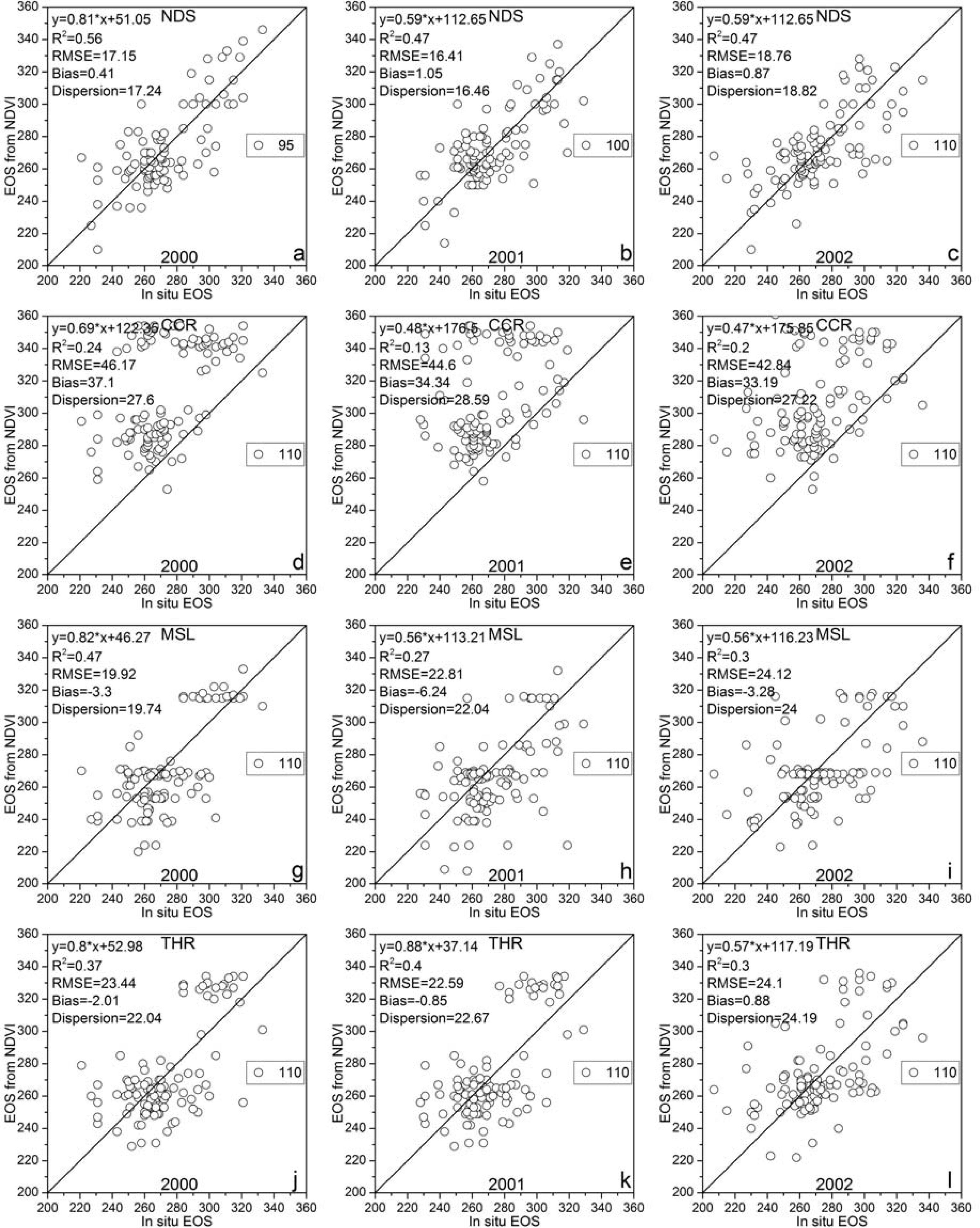
3.2. Accuracy Evaluation of Detection Results

Comparisons between the estimated SOS/EOS date based on remote sensing data and the in situ observation data from 110 stations for 2000–2002 are presented in Figures 6 and 7. SOS (Figure 6) and EOS (Figure 7) dates were estimated using the four different methods for threshold detection: (1) this study’s proposed NDS threshold method, (2) the curvature-change rate (CCR) method by Zhang et al. [13], (3) the maximum slope (MSL) method by Yu et al. [27], and the (4) threshold (THR) method by White and Nemani [22].

For SOS, the proposed NDS threshold method has the highest coefficient of determination (R²), smallest RMSE, and smallest dispersion among all four methods. Although the accuracy is not very high, the results still suggest that the proposed method can achieve a higher accuracy than the other methods on a national scale. Among the other three methods, the CCR method has the ability to treat each pixel individually without setting thresholds or empirical constants, allowing the method to be applied globally [13]. However, the CCR results, and in particular its high RMSE, suggest that although the method may work fine for vegetation, it is less applicable for crops in China. The MSL method also is a method that can be applied globally. The large positive bias of the MSL method, however, indicates that its estimated SOS tends to be much later than the observed dates for SOS. One reason for this is that the SOS from the in situ data represents the date of onset of photosynthetic activity, while the SOS derived by the MSL method corresponds to the time when the crop-growing rate is at a maximum, which is later than the onset of photosynthetic activity. The last method, the threshold method used by White and Nemani, is an empirical method that uses the halfway value between the minimum and maximum of annual NDVI curve as the threshold to detect phenology. The results (high RMSE), however, indicate that this method is not an accurate approach for phenology detection when used for crops across China.

For the detection of EOS dates, none of the four methods gives very good results, with low coefficients of determination and high RMSE for all four methods. One explanation can be that lower sun angles in autumn aggravate atmospheric effects [33]. Among the four methods, however, the NDS method still achieved the best results. The difference in results between the CCR and MSL methods might be explained by their different definitions of EOS. The EOS derived from the CCR method corresponds to the period when crop photosynthetic activity reaches zero [13]. For MSL, it corresponds to the onset of leaf coloring [33], which happens before photosynthetic activity reaches zero. Overall, on a national scale, the results of the CCR and MSL approaches and in particular the large bias for CCR results compared to MSL indicate that the EOS (as determined by the field observations) is closer to the date of onset of leaf coloring (used by the MSL method) than the end of photosynthetic activity (used by the CCR method).

The root mean square error (RMSE) of the various methods and the relative accuracies (RIA) of the NDS threshold method compared to the other three methods are presented in

Table 3. RMSE for all four methods and the relative accuracies (RIA) of NDS to the three other methods, for SOS and EOS.

			2000	2001	2002	Average
SOS	RMSE	NDS	18.95	16.79	15.67	17.14
		CCR	27.99	24.74	26.34	26.36
		MSL	33.27	29.03	34.21	32.17
		THR	27.1	24.66	26.3	26.02
	RIA	RIANDS,CCR	32.30%	32.13%	40.51%	34.98%
		RIANDS,MSL	43.04%	42.16%	54.19%	46.47%
		RIANDS,THR	30.07%	31.91%	40.42%	34.14%
EOS	RMSE	NDS	17.15	16.41	18.76	17.44
		CCR	46.17	44.6	42.84	44.54
		MSL	19.92	22.81	24.12	22.28
		THR	23.44	22.59	24.1	23.38
	RIA	RIANDS,CCR	62.85%	63.21%	56.21%	60.76%
		RIANDS,MSL	13.91%	28.06%	22.22%	21.40%
		RIANDS,THR	26.83%	27.36%	22.16%	25.45%

. The results show that for both SOS and EOS detection using remote sensing, use of the NDS threshold method can improve accuracy significantly. The average RMSE for the three years for the NDS method is smaller than 20 days for both SOS and EOS determination, while the RMSEs for the other three methods all exceed 20 days except for EOS of MSL in 2000. The average RIA of the NDS approach compared to the other methods also is above 30%, except for the relative accuracy of the NDS method compared to the MSL and THR methods when determining EOS.

In summary, in the case of China, the detection of both SOS and EOS based on remote sensing data can be improved by using the NDS threshold method proposed in this paper. Unlike the other methods, the new NDS method takes into consideration the variety in crop proportions and climate conditions across China by not using the same threshold for all zones. Both the CCR and MSL method detect phenological stages using geometric features of the NDVI curve, which is not reasonable for crop phenology detection across China because those features that will respond to SOS or EOS are not the same for different crops. Some crops even do not show any obvious geometric features in their NDVI curve when they reach SOS or EOS because of human activities. Unlike the CCR and MSL approaches, the NDS method does not consider the geometric features of the NDVI curve. Its thresholds are decided by the observed phenological stages, so it can bring the detected SOS/EOS dates closer to the real crop phenology. As a result, its findings are more accurate.

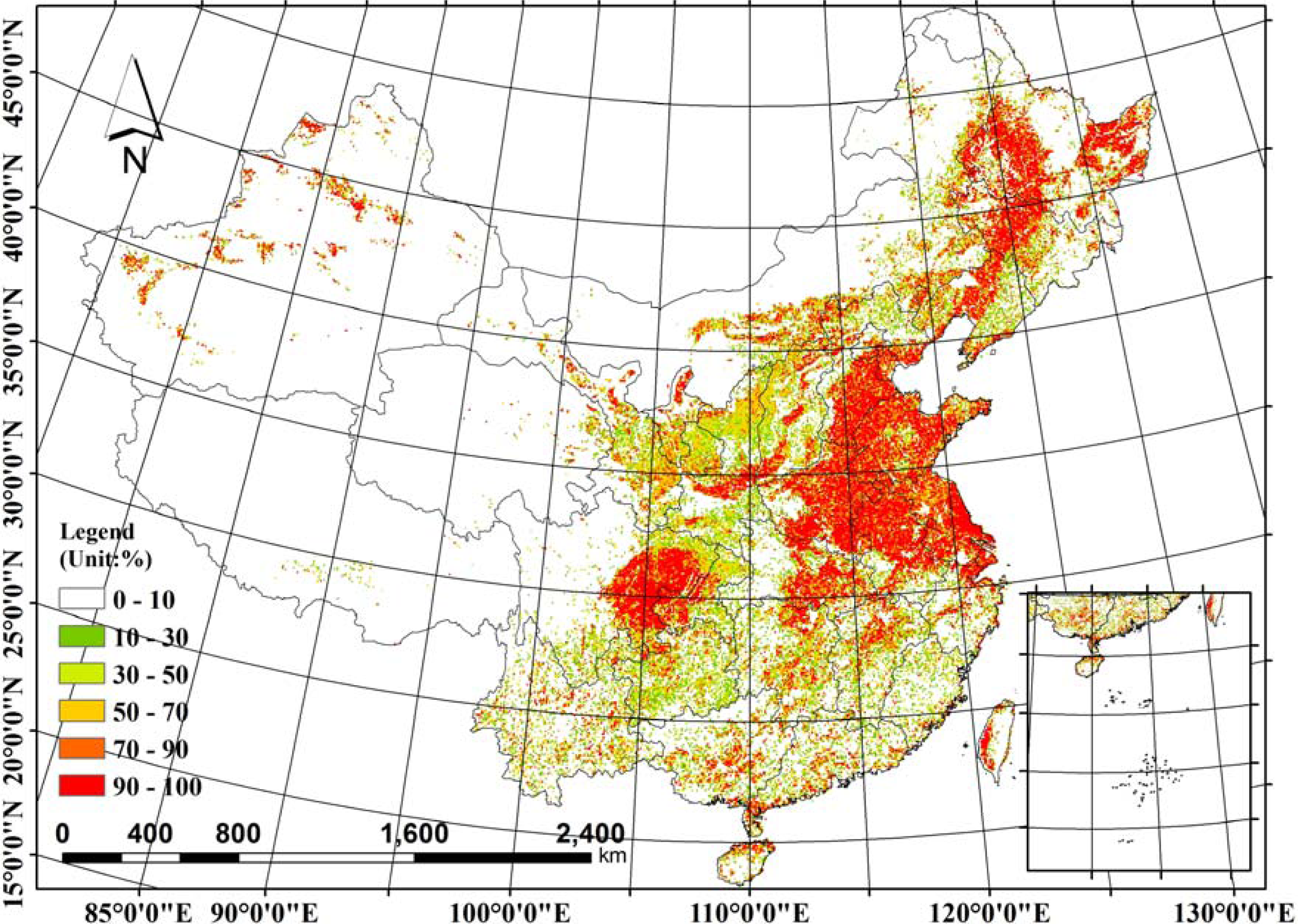
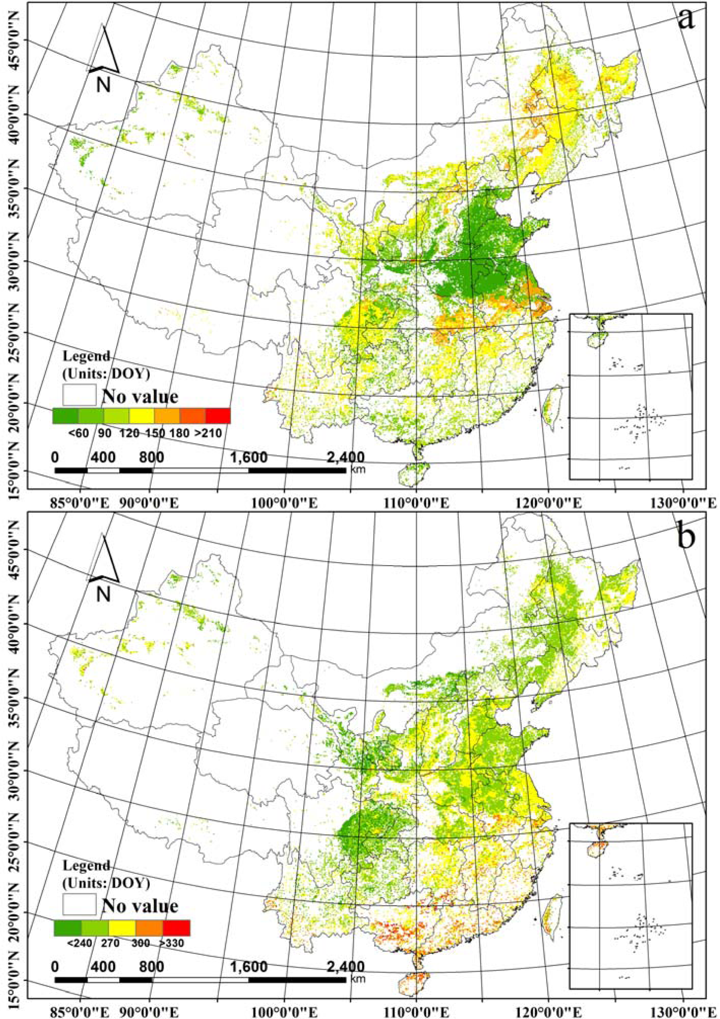
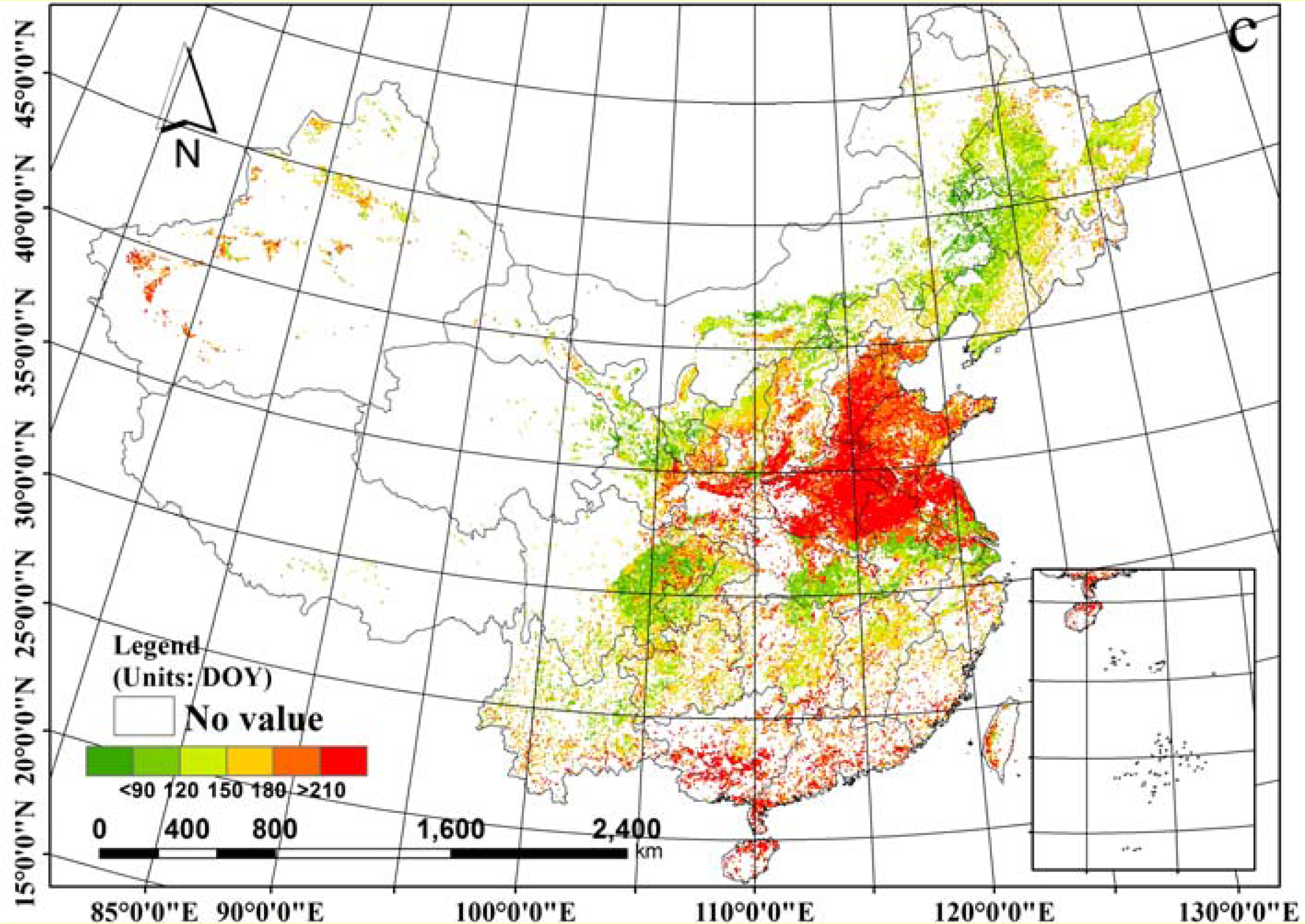
3.3. Maps of the Phenological Events

Figure 8 shows the start, end, and length (SOS, EOS, and LOS) of the growing season in 2002 as detected by the NDS method. In the case of denied pixels using the NDS method (pixels for which the value of N, S, and D did not yield acceptable results), the threshold method by White and Nemani [22] was used to determine the SOS and EOS.

Results shown in Figure 8 correspond with the fact that in China double cropping is predominantly located in the North China Plain, the middle and lower reaches of the Yangtze River, and the south of China [23], as double cropping leads to earlier SOS, later EOS, and longer LOS in those regions. Because of the physical environment and different crop types, regions with double cropping also do not show the same phenology. For example, in most regions of the North China Plain, the planting pattern is “winter wheat-summer corn”, while in most parts in the south of China the planting pattern is “early rice-late rice”. Usually, winter wheat’s SOS (its period of returning green) is earlier than the SOS of early rice (transplanting time). This can be seen in Figure 8(a) with earlier SOS in in the North China Plain compared with SOS in the South of China. Single cropping occurs throughout all cultivated areas in China, but is most common in the Northeast Plain, regions along the Great Wall of Inner Mongolia, the Loess Plateau, and Southwest China [23]. In these region relatively later SOS, earlier EOS, and shorter LOS have been observed.

3.4. Discussion of the Methodology

Although the method proposed in this study has shown to be an appropriate method for crop phenology detection in China, some problems remain.

First, to determine the detection thresholds for each zone, observation data must be available in that zone or in a nearby zone. This means that the method cannot be used in areas where observation data is not available. Moreover, the detection thresholds must be re-established after a certain period of time. Although it might be reasonable to assume that crop phenology is similar for three to five successive years, so that the same detection thresholds can be used, this consistency will certainly not apply to long-term monitoring. Global climate change in particular has shown in recent years to detrimentally affect many biological and environmental factors [37].

Second, the observed measurements of SOS/EOS and the estimated SOS/EOS based on remote sensing are in fact not very compatible because the observations are species-specific while the remote sensing data is not. In an eight-kilometer resolution image, each pixel reflects the integrated response across landscapes with diverse species and phenologic behavior, and it will affect the verification in this paper. The use of higher resolution data, such as MODIS data, would improve this situation as the smaller pixels would include fewer kinds of crop.

A third area that requires more attention is that the method proposed in this study assumes that within a zone planting patterns and environment do not vary significantly. This cannot always be the case and it is possible that results could be improved by increasing the total number of zones.

Finally, one aspect of the NDS method is the fact that the NDVI curve for some pixels does not lead to an acceptable SOS/EOS when the date falls outside the range of minimum to maximum SOS/EOS. Figure 9 shows the example of a pixel in zone 2–2 with N, S, D threshold values of 0.48, 0.022, and 0.171, respectively. For each threshold, the corresponding day of SOS falls outside the acceptable range for the zone, causing the pixel to not have an associated SOS. In this paper, the threshold method by White and Nemani [22] has been used to determine the SOS for those pixels to make the phenology maps in Figure 8, but more work needs to be done to find a better way to solve this situation.

4. Conclusions

This paper presents an improved threshold method for crop phenology detection in China based on remote sensing. Our method used field observed phenology data (SOS/EOS) in 2003 to derive the corresponding normalized difference vegetation index (NDVI or N) value, slope of the NDVI curve (S) value, and difference (D) between the NDVI value and a base NDVI value for every agro-meteorological station. For each of 43 agricultural zones with different crop proportions, we designed an algorithm to establish an optimal set of detection thresholds (N, S and D), which can achieve the highest percentage of accepted pixels (PA) for SOS and EOS of each zone.

Verification results showed a relative good agreement between in situ SOS dates and the SOS dates based on remote sensing data using the proposed method. The average root mean square error (2000–2002) of SOS and EOS is 17.14 days and 17.44 days, respectively. The comparisons demonstrated that our method showed higher accuracy than three other methods based on remote sensing data. Compared with curvature-change rate method (CCR) described by Zhang et al. [13], maximum slope (MSL) method used by Yu et al. [27], and threshold method (THR) by White and Nemani [22], the method proposed in this study can improve the average accuracy (2000–2002) by about 35%, 46%, and 34% for SOS, about 61%, 21%, and 25% for EOS, respectively. In addition, maps of the phenological events showed a good agreement with the previous study.

The primary innovations of our method are twofold. First, we proposed a method for crop phenology detection. As crop is often affected by human activities, it is difficult to detect its phenology using ordinary method. Using field observed data to derive the thresholds and then establishing the set of detection thresholds can eliminate some human activities’ influence. Second, we set different phenology detection thresholds for different agricultural zones, which is more reasonable for complex planting condition in China.

A limitation of the proposed method is that observation data needs to be available for study area and the thresholds will periodically need to be determined. In addition, our method will result in some pixels with no detectable phenological events. In future, further research is necessary to address these limitations. Verification method and agricultural zones dividing method also need to be further improved. After that, the method will be used to detect the crop phenology variation across China over the last 30 years for the study of the impact of climate change on crops.

References

1. Sakamoto, T.; Yokozawa, M.; Toritani, H.; Shibayama, M.; Ishitsuka, N.; Ohno, H. A crop phenology detection method using time-series modis data. Remote Sens. Environ 2005, 96, 366–374. [Google Scholar]
2. Thenkabail, P.S. Global croplands and their importance for water and food security in the twenty-first century: Towards an ever green revolution that combines a second green revolution with a blue revolution. Remote Sens 2010, 2, 2305–2312. [Google Scholar]
3. Becker-Reshef, I.; Justice, C.; Sullivan, M.; Vermote, E.; Tucker, C.; Anyamba, A.; Small, J.; Pak, E.; Masuoka, E.; Schmaltz, J.; et al. Monitoring global croplands with coarse resolution earth observations: The global agriculture monitoring (glam) project. Remote Sens 2010, 2, 1589–1609. [Google Scholar]
4. Cong, N.; Piao, S.; Chen, A.; Wang, X.; Lin, X.; Chen, S.; Han, S.; Zhou, G.; Zhang, X. Spring vegetation green-up date in china inferred from spot NDVI data: A multiple model analysis. Agric. For. Meteorol 2012, 165, 104–113. [Google Scholar]
5. Savitzky, A.; Golay, M. Smoothing and differentiation of data by simplified least squares procedures. Anal. Chem 1964, 36, 1627–1639. [Google Scholar]
6. Chen, J.; Jönsson, P.; Tamura, M.; Gu, Z.; Matsushita, B.; Eklundh, L. A simple method for reconstructing a high-quality NDVI time-series data set based on the Savitzky–Golay filter. Remote Sens. Environ 2004, 91, 332–344. [Google Scholar]
7. Hird, J.N.; McDermid, G.J. Noise reduction of NDVI time series: An empirical comparison of selected techniques. Remote Sens. Environ 2009, 113, 248–258. [Google Scholar]
8. White, M.A.; De Beurs, K.M.; Didan, K.; Inouye, D.W.; Richardson, A.D.; Jensen, O.P.; O’Keefe, J.; Zhang, G.; Nemani, R.R.; van Leeuwen, W.J.D.; et al. Intercomparison, interpretation, and assessment of spring phenology in North America estimated from remote sensing for 1982–2006. Glob. Change Biol 2009, 15, 2335–2359. [Google Scholar]
9. Beck, P.S.A.; Atzberger, C.; Høgda, K.A.; Johansen, B.; Skidmore, A.K. Improved monitoring of vegetation dynamics at very high latitudes: A new method using modis NDVI. Remote Sens. Environ 2006, 100, 321–334. [Google Scholar]
10. Atkinson, P.M.; Jeganathan, C.; Dash, J.; Atzberger, C. Inter-comparison of four models for smoothing satellite sensor time-series data to estimate vegetation phenology. Remote Sens. Environ 2012, 123, 400–417. [Google Scholar]
11. Jönsson, P.; Eklundh, L. Seasonality extraction by function fitting to time-series of satellite sensor data. IEEE Trans. Geosci. Remot. Sens 2002, 40, 1824–1832. [Google Scholar]
12. Roerink, G.J.; Menenti, M.; Soepboer, W.; Su, Z. Assessment of climate impact on vegetation dynamics by using remote sensing. Phys. Chem. Earth 2003, 28, 103–109. [Google Scholar]
13. Zhang, X.; Friedl, M.A.; Schaaf, C.B.; Strahler, A.H.; Hodges, J.C.F.; Gao, F.; Reed, B.C.; Huete, A. Monitoring vegetation phenology using MODIS. Remote Sens. Environ 2003, 84, 471–475. [Google Scholar]
14. Eilers, P.H.C. A perfect smoother. Anal. Chem 2003, 75, 3631–3636. [Google Scholar]
15. Atzberger, C.; Eilers, P.H.C. A time series for monitoring vegetation activity and phenology at 10-daily time steps covering large parts of South America. Int. J. Digit. earth 2011, 4, 365–386. [Google Scholar]
16. Atzberger, C.; Eilers, P.H.C. Evaluating the effectiveness of smoothing algorithms in the absence of ground reference measurements. Int. J. Remote Sens 2011, 32, 3689–3709. [Google Scholar]
17. Hermance, J.F.; Jacob, R.W.; Bradley, B.A.; Mustard, J.F. Extracting phenological signals from multiyear AVHRR NDVI time series: Framework for applying high-order annual splines with roughness damping. IEEE Trans. Geosci. Remote Sens 2007, 45, 3264–3276. [Google Scholar]
18. Zhu, W.; Pan, Y.; He, H.; Wang, L.; Mou, M.; Liu, J. A changing-weight filter method for reconstructing a high-quality NDVI time series to preserve the integrity of vegetation phenology. IEEE Trans. Geosci. Remote Sens 2012, 50, 1085–1094. [Google Scholar]
19. Jeong, S.J.; Ho, C.H.; Gim, H.J.; Brown, M.E. Phenology shifts at start vs. end of growing season in temperate vegetation over the Northern Hemisphere for the period 1982–2008. Glob. Change Biol 2011, 17, 2385–2399. [Google Scholar]
20. Lloyd, D. Phenological classification of terrestrial vegetation cover using shortwave vegetation index imagery. Int. J. Remote Sens 1990, 11, 2269–2279. [Google Scholar]
21. Delbart, N.; Le Toan, T.; Kergoat, L.; Fedotova, V. Remote sensing of spring phenology in boreal regions: A free of snow-effect method using NOAA-AVHRR and SPOT-VGT data (1982–2004). Remote Sens. Environ 2006, 101, 52–62. [Google Scholar]
22. White, M.A.; Nemani, R.R. Real-time monitoring and short-term forecasting of land surface phenology. Remote Sens. Environ 2006, 104, 43–49. [Google Scholar]
23. Wu, W.; Yang, P.; Tang, H.; Zhou, Q.; Chen, Z.; Shibasaki, R. Characterizing spatial patterns of phenology in cropland of China based on remotely sensed data. J. Integr. Agric 2010, 9, 101–112. [Google Scholar]
24. Moody, A.; Johnson, D.M. Land-surface phenologies from AVHRR using the discrete fourier transform. Remote Sens. Environ 2001, 75, 305–323. [Google Scholar]
25. Reed, B.C.; Brown, J.F.; VanderZee, D.; Loveland, T.R.; Merchant, J.W.; Ohlen, D.O. Measuring phenological variability from satellite imagery. J. Veg. Sci 1994, 5, 703–714. [Google Scholar]
26. Duchemin, B.T.; Goubier, J.; Courrier, G. Monitoring phenological key stages and cycle duration of temperate deciduous forest ecosystems with NOAA/AVHRR data. Remote Sens. Environ 1999, 67, 68–82. [Google Scholar]
27. Yu, F.; Kevin, P.P.; James, E.; Shi, P. Response of seasonal vegetation development to climatic variations in Eastern Central Asia. Remote Sens. Environ 2003, 87, 42–54. [Google Scholar]
28. Dash, J.; Jeganathan, C.; Atkinson, P.M. The use of MERIS terrestrial chlorophyll index to study spatio-temporal variation in vegetation phenology over India. Remote Sens. Environ. 2010, 1388–1402. [Google Scholar]
29. Pan, Y.; Li, L.; Zhang, J.; Liang, S.; Zhu, X.; Sulla-Menashe, D. Winter wheat area estimation from MODIS-EVI time series data using the crop proportion phenology index. Remote Sens. Environ 2012, 119, 232–242. [Google Scholar]
30. Kaufmann, R.K.; Zhou, L.; Knyazikhin, Y.; Shabanov, N.V.; Tucker, C.J. Effect of orbital drift and sensor changes on the time series of AVHRR vegetation index data. IEEE Trans. Geosci. Remote Sens 2000, 38, 2584–2597. [Google Scholar]
31. Liu, J.; Liu, M.; Tian, H.; Zhuang, D.; Zhang, Z.; Zhang, W.; Tang, X.; Deng, X. Spatial and temporal patterns of china’s cropland during 1990–2000: An analysis based on Landsat TM data. Remote Sens. Environ 2005, 98, 442–456. [Google Scholar]
32. Meng, J.; Wu, B.; Li, Q. Method for estimating crop leaf area index of China using remote sensing (in Chinese). Trans. CSAE 2007, 23, 160–167. [Google Scholar]
33. Delbart, N.; Kergoat, L.; Le Toan, T.; Lhermitte, J.; Picard, G. Determination of phenological dates in boreal regions using normalized difference water index. Remote Sens. Environ 2005, 97, 26–38. [Google Scholar]
34. Zhang, F.; Wu, B.; Liu, C.; Luo, Z. Methods of monitoring crop phenological stages using time series of vegetation indicator (in Chinese). Trans. CSAE 2004, 20, 138–143. [Google Scholar]
35. Schwarts, M.D.; Reed, B.C. Surface phenology and satellite sensor-derived onset of greenness: An initial comparison. Int. J. Remote Sens 1999, 20, 3451–3457. [Google Scholar]
36. Willmott, C.J. Some comments on the evaluation of model performance. Bull. Amer. Meteorol. Soc 1982, 63, 1390–1313. [Google Scholar]
37. Kang, J.X. Omega-3: A link between global climate change and human health. Biotechnol. Adv 2011, 29, 388–390. [Google Scholar]
Figure 1. Map of cropland density in China at a resolution of 8 km.
Remotesensing 05 03190f1
Figure 2. Map of agro-meteorological stations and crop proportion zones in China. W = wheat, Spr. W = spring wheat, Win. W = winter wheat, M = maize, Spr. M = spring maize, Sum. M = summer maize, R = rice, S = soybean.
Remotesensing 05 03190f2
Figure 3. Study methodology consisting of (1) data preprocessing, (2) determination of phenology detection thresholds, and (3) verification and comparison.
Remotesensing 05 03190f3
Figure 4. Deriving values for NDVI (N), Slope (S), and Difference (D) for each agro-meteorological station based on the observed start of the growing season (SOS) or end of the growing season (EOS).
Remotesensing 05 03190f4
Figure 5. Algorithm for determining phenology detection thresholds.
Remotesensing 05 03190f5
Figure 6. Comparisons of in situ SOS date (DOY) with SOS date (DOY) derived from four methods based on remote sensing data: (ac) This study’s NDS method; (df) Curvature-change rate method; (gi) Maximum slope method; (jl) Threshold method.
Remotesensing 05 03190f6
Figure 7. Comparisons of in situ EOS date (DOY) with EOS date (DOY) derived from four methods based on remote sensing data: (ac) This study’s NDS method; (df) Curvature-change rate method; (gi) Maximum slope method; (jl) Threshold method.
Remotesensing 05 03190f7
Figure 8. Maps of the (a) SOS; (b) EOS; and (c) LOS (DOY) in China, 2002.
Remotesensing 05 03190f8aRemotesensing 05 03190f8b
Figure 9. NDVI, slope, and difference curves for a pixel with no detectable SOS value. N = NDVI; S = Slope; D = Difference. The horizontal lines represent the detection thresholds for N, S, and D. The dotted vertical lines show the minimum (left) and maximum (right) days for the SOS. For all three thresholds, the day of the SOS corresponding to the threshold falls outside the range of SOS dates. The pixel does not provide an acceptable result and is denied.
Remotesensing 05 03190f9