Can Night-Time Light Data Identify Typologies of Urbanization? A Global Assessment of Successes and Failures

Abstract
:1. Introduction
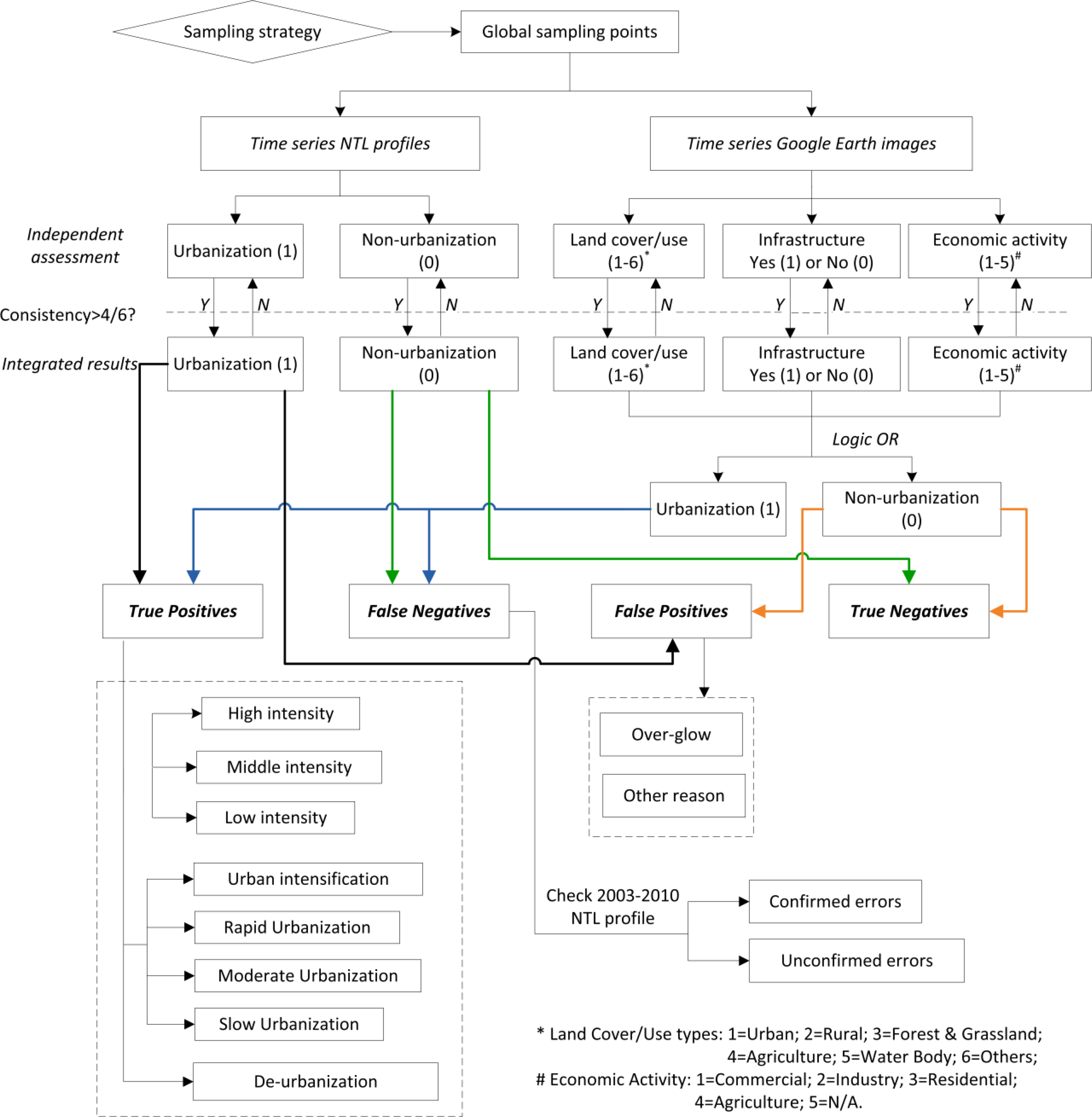
2. Methodology
2.1. Data and General Procedures
2.2. Labeling and Interpretation
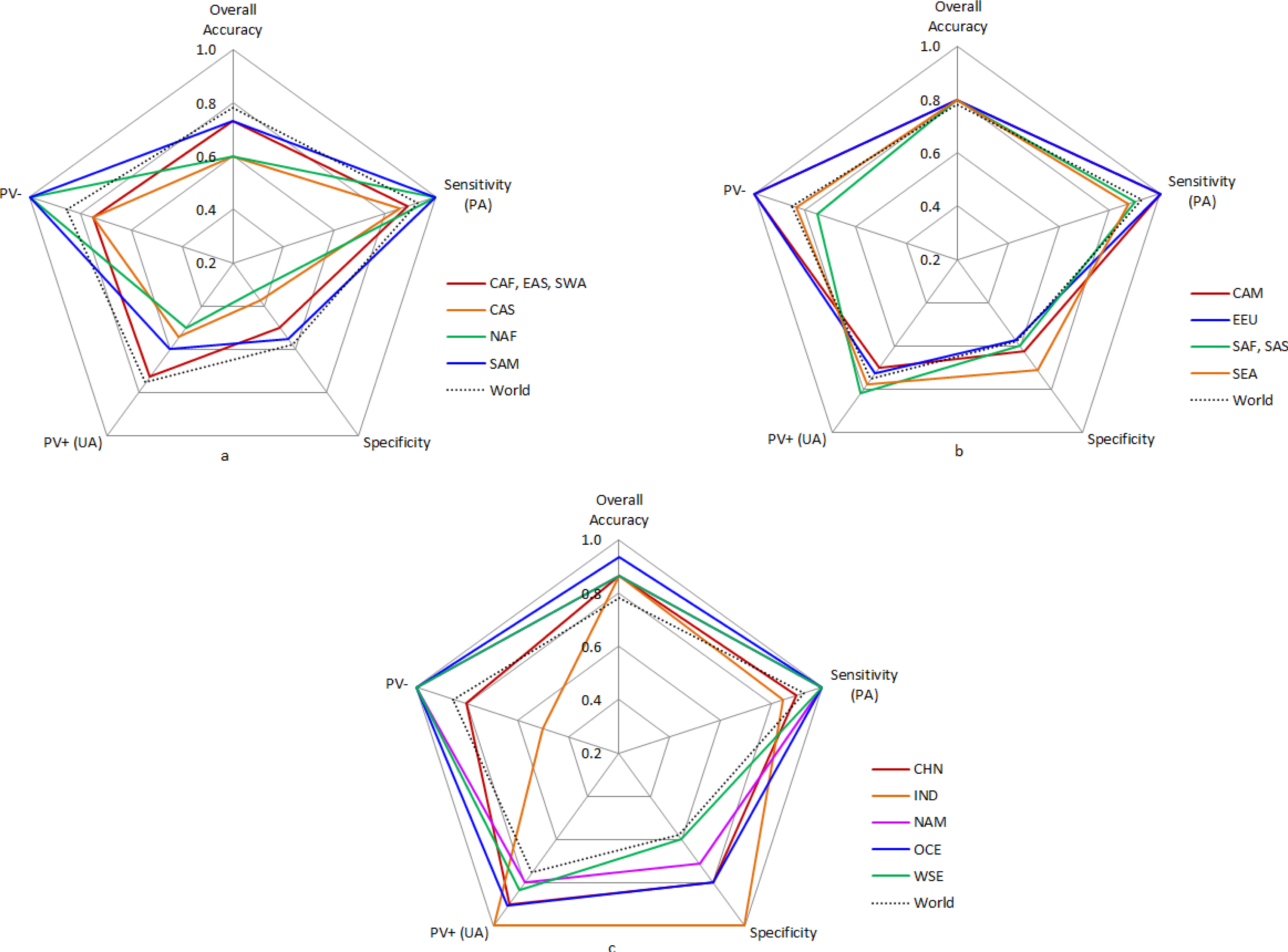
2.3. Quantitative Indicators
3. Results and Discussion
3.1. Overall Accuracy
3.2. Successes: True Positives and True Negatives
3.3. Failures: False Positives and False Negatives
4. Conclusions
Acknowledgments
Conflict of Interest
References
- Batty, M. The size, scale, and shape of cities. Science 2008, 319, 769–771. [Google Scholar]
- Lankao, P.R.; Nychka, D.; Tribbia, J.L. Development and greenhouse gas emissions deviate from the “modernization” theory and “convergence” hypothesis. Clim. Res 2008, 38, 17–29. [Google Scholar]
- Mumford, L. The City in History: Its Origins, Its Transformations, and Its Prospects; Harcourt, Brace & World: New York, NY, USA, 1961; p. 794. [Google Scholar]
- Montgomery, M.R.; Stren, R.; Cohen, B.; Reed, H.E. Cities Transformed: Demographic Change and Its Implications in the Developing World; The National Academies Press: Washington, DC, USA, 2003; p. 552. [Google Scholar]
- Weber, M. The City; Free Press: New York, NY, USA, 1966; p. 252. [Google Scholar]
- Davis, J.C.; Henderson, J.V. Evidence on the political economy of the urbanization process. J. Urban Econ 2003, 53, 98–125. [Google Scholar]
- Henderson, V. The urbanization process and economic growth: The so-what question. J. Econ. Growth 2003, 8, 47–71. [Google Scholar]
- Schneider, A.; Friedl, M.A.; Potere, D. A new map of global urban extent from modis satellite data. Environ. Res. Lett 2009, 4, 044003. [Google Scholar]
- Seto, K.C.; Fragkias, M.; Güneralp, B.; Reilly, M.K. A meta-analysis of global urban land expansion. PLoS One 2011, 6, e23777. [Google Scholar]
- Baugh, K.; Elvidge, C.; Ghosh, T.; Ziskin, D. Development of a 2009 Stable Lights Product Using DMSP-OLS Data. Proceedings of the 30th Asia-Pacific Advanced Network Meeting, Hanoi, Vietnam, 9–10 August 2010; pp. 114–130.
- Chen, X.; Nordhaus, W.D. Using luminosity data as a proxy for economic statistics. Proc. Natl. Acad. Sci. USA 2011, 108, 8589–8594. [Google Scholar]
- Henderson, J.V.; Storeygard, A.; Weil, D.N. Measuring economic growth from outer space. Am. Econ. Rev 2012, 102, 994–1028. [Google Scholar]
- Sutton, P.C.; Elvidge, C.D.; Ghosh, T. Estimation of gross domestic product at sub-national scales using nighttime satellite imagery. Int. J. Ecol. Econ. Stat 2007, 8, 5–21. [Google Scholar]
- Sutton, P.; Roberts, D.; Elvidge, C.; Baugh, K. Census from heaven: An estimate of the global human population using night-time satellite imagery. Int. J. Remote Sens 2001, 22, 3061–3076. [Google Scholar]
- Sutton, P.C.; Elvidge, C.; Obremski, T. Building and evaluating models to estimate ambient population density. Photogramm. Eng. Remote Sensing 2003, 69, 545–553. [Google Scholar]
- Zhuo, L.; Ichinose, T.; Zheng, J.; Chen, J.; Shi, P.J.; Li, X. Modelling the population density of china at the pixel level based on DMSP/OLS non–radiance–calibrated night-time light images. Int. J. Remote Sens 2009, 30, 1003–1018. [Google Scholar]
- Elvidge, C.D.; Imhoff, M.L.; Baugh, K.E.; Hobson, V.R.; Nelson, I.; Safran, J.; Dietz, J.B.; Tuttle, B.T. Night-time lights of the world: 1994–1995. ISPRS J. Photogramm 2001, 56, 81–99. [Google Scholar]
- Elvidge, C.D.; Tuttle, B.T.; Sutton, P.C.; Baugh, K.E.; Howard, A.T.; Milesi, C.; Bhaduri, B.; Nemani, R. Global distribution and density of constructed impervious surfaces. Sensors 2007, 7, 1962–1979. [Google Scholar]
- Lu, D.; Tian, H.; Zhou, G.; Ge, H. Regional mapping of human settlements in Southeastern China with multisensor remotely sensed data. Remote Sens. Environ 2008, 112, 3668–3679. [Google Scholar]
- Ma, T.; Zhou, C.; Pei, T.; Haynie, S.; Fan, J. Quantitative estimation of urbanization dynamics using time series of dmsp/ols nighttime light data: A comparative case study from China’s cities. Remote Sens. Environ 2012, 124, 99–107. [Google Scholar]
- Elvidge, C.; Safran, J.; Nelson, I.; Tuttle, B.; Ruth Hobson, V.; Baugh, K.; Dietz, J.; Erwin, E. Area and Positional Accuracy of Dmsp Nighttime Lights Data. In Remote Sensing and GIS Accuracy Assessment; Lunetta, R., Lyon, J., Eds.; CRC Press: Boca Raton, FL, USA, 2004; pp. 281–292. [Google Scholar]
- Henderson, M.; Yeh, E.T.; Gong, P.; Elvidge, C.; Baugh, K. Validation of urban boundaries derived from global night-time satellite imagery. Int. J. Remote Sens 2003, 24, 595–609. [Google Scholar]
- Levin, N.; Duke, Y. High spatial resolution night-time light images for demographic and socio-economic studies. Remote Sens. Environ 2012, 119, 1–10. [Google Scholar]
- Small, C.; Elvidge, C.D.; Balk, D.; Montgomery, M. Spatial scaling of stable night lights. Remote Sens. Environ 2011, 115, 269–280. [Google Scholar]
- Small, C.; Pozzi, F.; Elvidge, C.D. Spatial analysis of global urban extent from DMSP-OLS night lights. Remote Sens. Environ 2005, 96, 277–291. [Google Scholar]
- Tuttle, B.T.; Anderson, S.J.; Sutton, P.C.; Elvidge, C.D.; Kim, B. It used to be dark here: Geolocation calibration of the defense meteorological satellite program operational linescan system. Photogramm. Eng. Remote Sensing 2013, 79, 287–297. [Google Scholar]
- Liu, Z.; He, C.; Zhang, Q.; Huang, Q.; Yang, Y. Extracting the dynamics of urban expansion in china using DMSP-OLS nighttime light data from 1992 to 2008. Landsc. Urban Plan 2012, 106, 62–72. [Google Scholar]
- Small, C.; Elvidge, C.D. Night on earth: Mapping decadal changes of anthropogenic night light in asia. Int. J. Appl. Earth Observ. Geoinf 2013, 22, 40–52. [Google Scholar]
- Zhang, Q.; Seto, K.C. Mapping urbanization dynamics at regional and global scales using multi-temporal dmsp/ols nighttime light data. Remote Sens. Environ 2011, 115, 2320–2329. [Google Scholar]
- Sutton, P.C.; Taylor, M.J.; Anderson, S.; Elvidge, C.D. Sociodemographic Characterization of Urban Areas Using Nighttime Imagery, Google Earth, Landsat, and “Social” Ground Truthing in Urban Remote Sensing. In Urban Remote Sensing; Weng, Q., Quattrochi, D.A., Eds.; CRC Press: Boca Raton, FL, USA, 2007; pp. 291–310. [Google Scholar]
- Version 4 DMSP-OLS Nighttime Lights Time Series. Available online: http://www.ngdc.noaa.gov/eog/dmsp/downloadV4composites.html (accessed on 29 March 2013).
- Elvidge, C.D.; Ziskin, D.; Baugh, K.E.; Tuttle, B.T.; Ghosh, T.; Pack, D.W.; Erwin, E.H.; Zhizhin, M. A fifteen year record of global natural gas flaring derived from satellite data. Energies 2009, 2, 595–622. [Google Scholar]
- Seto, K.C.; Güneralp, B.; Hutyra, L.R. Global forecasts of urban expansion to 2030 and direct impacts on biodiversity and carbon pools. Proc. Natl. Acad. Sci. USA 2012, 109, 16083–16088. [Google Scholar]
- Congalton, R.G. A review of assessing the accuracy of classifications of remotely sensed data. Remote Sens. Environ 1991, 37, 35–46. [Google Scholar]
- Bland, M. An Introduction to Medical Statistics, 3rd ed.; Oxford University Press: Oxford, UK, 2000; p. 405. [Google Scholar]
- Lalkhen, A.G.; McCluskey, A. Clinical tests: Sensitivity and specificity. Contin. Educ. Anaesth. Crit. Care Pain 2008, 8, 221–223. [Google Scholar]
- Hastie, T.; Tibshirani, R.; Friedman, J.H. The Elements of Statistical Learning; Springer: New York, NY, USA, 2003; p. 552. [Google Scholar]
- Liu, J.; Liu, M.; Zhuang, D.; Zhang, Z.; Deng, X. Study on spatial pattern of land-use change in china during 1995–2000. Sci. China Ser. D-Earth Sci 2003, 46, 373–384. [Google Scholar]
- Liu, J.; Tian, H.; Liu, M.; Zhuang, D.; Melillo, J.M.; Zhang, Z. China’s changing landscape during the 1990s: Large-scale land transformations estimated with satellite data. Geophys. Res. Lett 2005, 32, L02405. [Google Scholar]
- Elvidge, C.D.; Baugh, K.E.; Sutton, P.C.; Bhaduri, B.; Tuttle, B.T.; Ghosh, T.; Ziskin, D.; Erwin, E.H. Who’s in the Dark—Satellite Based Estimates of Electrification Rates. In Urban Remote Sensing; Yang, X., Ed.; John Wiley & Sons, Ltd: Chichester, UK, 2011; pp. 211–224. [Google Scholar]
- Yep, E. Power problems threaten growth in India. The Wall Street Journal, 3 January 2012. [Google Scholar]
- Agency, I.E. World Energy Outlook 2011: Energy for All; International Energy Agency (IEA): Paris, France, 2011. [Google Scholar]
- Remme, U.; Trudeau, N.; Graczyk, D.; Taylor, P. Technology Development Prospects for the Indian Power Sector; International Energy Agency (IEA): Paris, France, 2011. [Google Scholar]


| Region | Abbreviation | Included UN Regions | Plus | Minus |
|---|---|---|---|---|
| Central America | CAM | Central America, Caribbean | – | – |
| China | CHN | – | China, Hong Kong, Macao | – |
| Eastern Asia | EAS | Eastern Asia | Taiwan | China, Hong Kong, Macao, Mongolia |
| Eastern Europe | EEU | Eastern Europe | Kazakhstan, Estonia, Lithuania, Latvia, Albania, Bosnia-Herzegovina, Croatia, Macedonia, Montenegro, Serbia | – |
| India | IND | – | India | – |
| Mid-Asia | MAS | Central Asia | Mongolia | Kazakhstan |
| Mid-Latitudinal Africa | MLA | Western, Middle, Eastern Africa | – | – |
| Northern Africa | NAF | Northern Africa | – | – |
| Northern America | NAM | Northern America | – | – |
| Oceania | OCE | Oceania | – | – |
| Southern Africa | SAF | Southern Africa | – | – |
| South America | SAM | Southern America | – | – |
| Southern Asia | SAS | Southern Asia | – | India |
| Southeastern Asia | SEA | Southeastern Asia | – | – |
| Western Asia | WAS | Western Asia | – | – |
| Western Europe | WSE | Western, Southern, and Northern Europe | – | Estonia, Lithuania, Latvia, Albania, Bosnia-Herzegovina, Croatia, Macedonia, Montenegro, Serbia |
| No | Indicator | Equation | Implication |
|---|---|---|---|
| 1 | Overall accuracy | the overall accuracy of time series NTL profile for identifying a particular urbanization typology | |
| 2 | Sensitivity | the ability of the NTL profile to correctly identify urbanization | |
| 3 | Specificity | the ability of the NTL profile to correctly identify the absence of urbanization | |
| 4 | Predictive value for a positive result (PV+) | How likely is the pixel experienced urbanization, given that the NTL profile shows urbanization-related signatures? | |
| 5 | Predictive value for a negative result (PV−) | How likely is the pixel did not experience urbanization, given that the NTL profile suggests an absence of urbanization-related signature? |
| Consistency | Land Cover/Use | Infrastructure | Economic Activity | NTL Profile |
|---|---|---|---|---|
| 100% (6/6) | 35.9% | 54.7% | 42.2% | 81.3% |
| 83.3% (5/6) | 42.8% | 29.7% | 39.0% | 15.6% |
| 66.7% (4/6) | 21.3% | 15.6% | 18.8% | 3.1% |
| High Constant Urban Economic Activities | Rapid Urbanization | |
|---|---|---|
| Time series NTL profile | 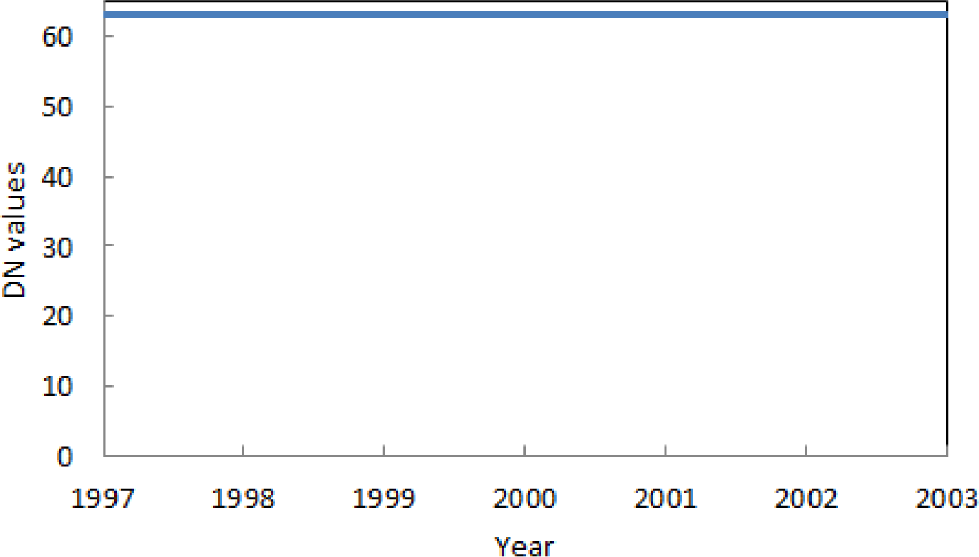 | 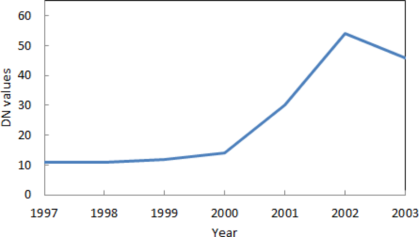 |
| Time series Google Earth images (1 km × 1 km) |  1944-12-31 | 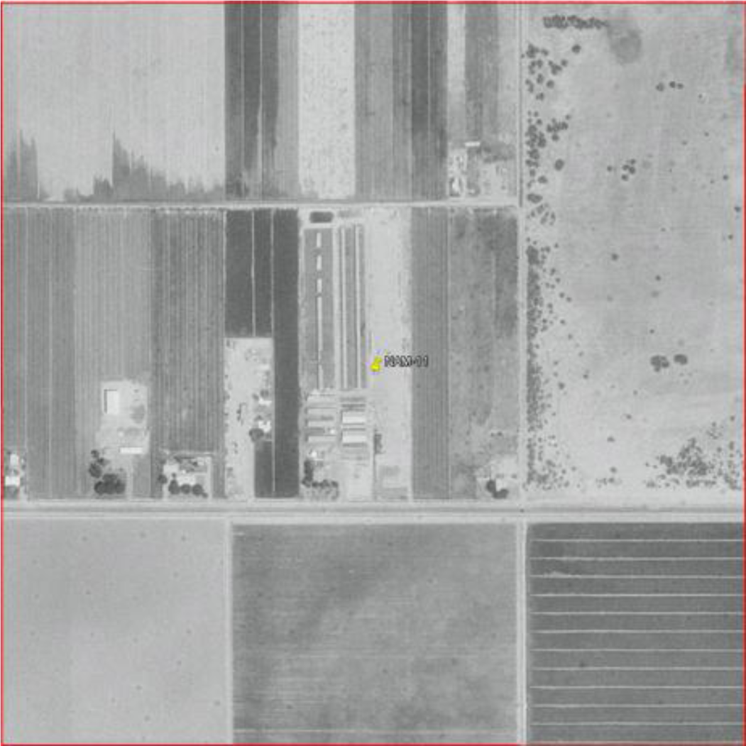 1997-04-29 |
 2002-07-18 | 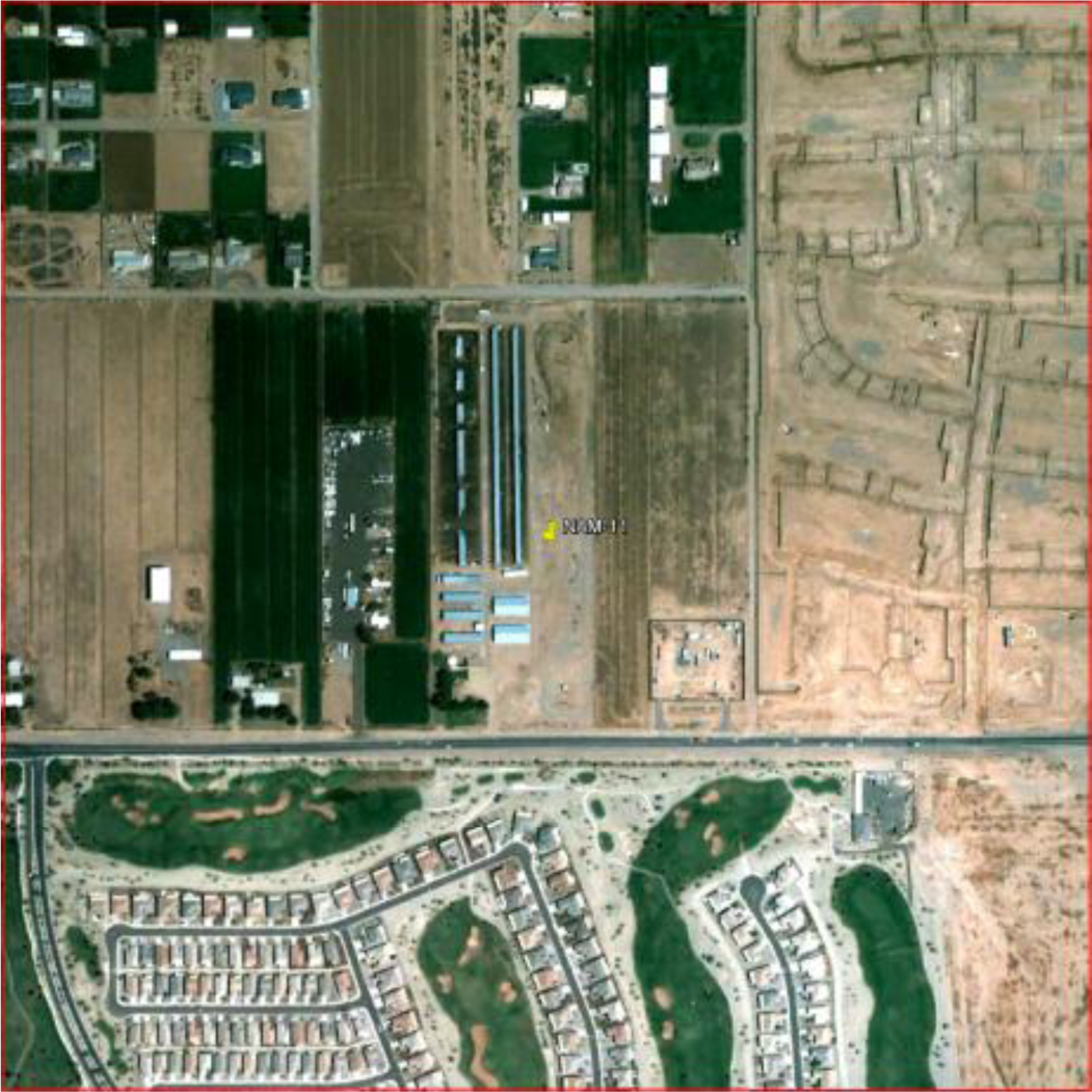 2003-09-05 |
| High CUEA | Medium CUEA | Low CUEA | Urbanization Intensification | Rapid Urbanization | Moderate Urbanization | Slow Urbanization | De-Urbanization | |
|---|---|---|---|---|---|---|---|---|
| CAM | ✓ | ✓ | ✓ | ✓ | ✓ | |||
| CHN | ✓ | ✓ | ✓ | ✓ | ||||
| EAS | ✓ | ✓ | ✓ | ✓ | ||||
| EEU | ✓ | ✓ | ✓ | ✓ | ✓ | ✓ | ||
| IND | ✓ | ✓ | ✓ | ✓ | ✓ | |||
| MAS | ✓ | ✓ | ✓ | ✓ | ||||
| MLA | ✓ | ✓ | ✓ | ✓ | ✓ | ✓ | ||
| NAF | ✓ | ✓ | ✓ | ✓ | ||||
| NAM | ✓ | ✓ | ✓ | ✓ | ✓ | |||
| OCE | ✓ | ✓ | ✓ | ✓ | ||||
| SAF | ✓ | ✓ | ✓ | ✓ | ✓ | |||
| SAM | ✓ | ✓ | ✓ | |||||
| SAS | ✓ | ✓ | ✓ | ✓ | ✓ | |||
| SEA | ✓ | ✓ | ✓ | ✓ | ✓ | ✓ | ||
| WAS | ✓ | ✓ | ✓ | ✓ | ✓ | |||
| WSE | ✓ | ✓ | ✓ | ✓ | ✓ |
| Time Series NTL Profile | Time Series Google Earth Images (1 km × 1 km) | |
|---|---|---|
| False Negatives |  | 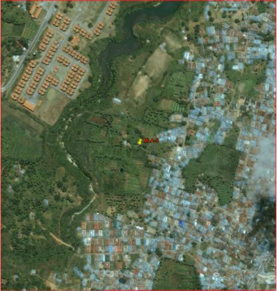 2003-09-22 |
| False Positives | 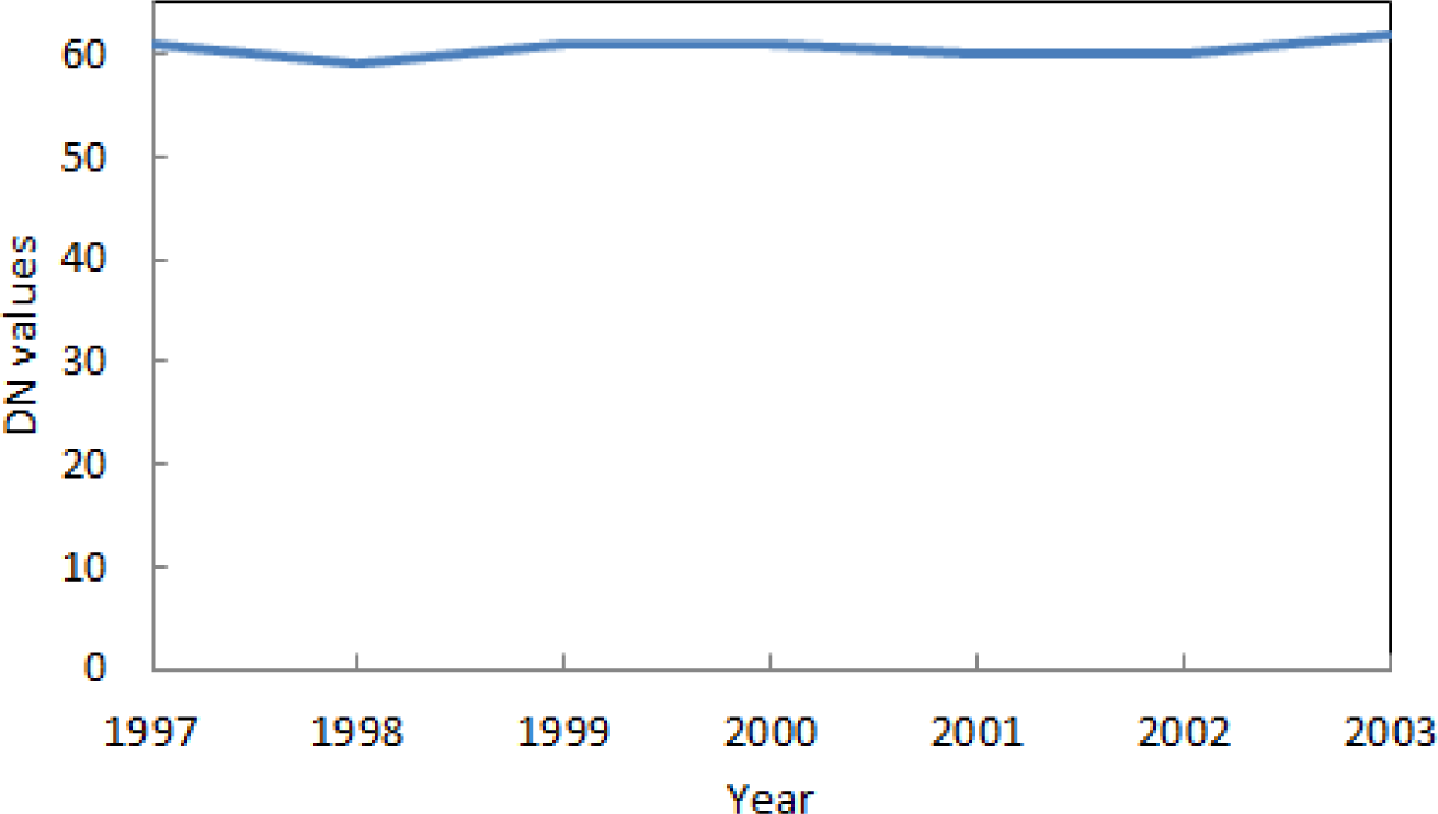 |  2002-06-07 |
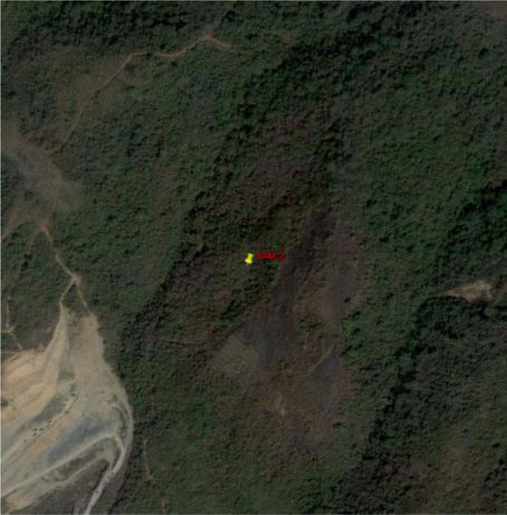 2003-12-29 |
© 2013 by the authors; licensee MDPI, Basel, Switzerland This article is an open access article distributed under the terms and conditions of the Creative Commons Attribution license (http://creativecommons.org/licenses/by/3.0/).
Share and Cite
Zhang, Q.; Seto, K.C. Can Night-Time Light Data Identify Typologies of Urbanization? A Global Assessment of Successes and Failures. Remote Sens. 2013, 5, 3476-3494. https://doi.org/10.3390/rs5073476
Zhang Q, Seto KC. Can Night-Time Light Data Identify Typologies of Urbanization? A Global Assessment of Successes and Failures. Remote Sensing. 2013; 5(7):3476-3494. https://doi.org/10.3390/rs5073476
Chicago/Turabian StyleZhang, Qian, and Karen C. Seto. 2013. "Can Night-Time Light Data Identify Typologies of Urbanization? A Global Assessment of Successes and Failures" Remote Sensing 5, no. 7: 3476-3494. https://doi.org/10.3390/rs5073476