Soil Moisture & Snow Properties Determination with GNSS in Alpine Environments: Challenges, Status, and Perspectives

Abstract

Moisture content in the soil and snow in the alpine environment is an important factor, not only for environmentally oriented research, but also for decision making in agriculture and hazard management. Current observation techniques quantifying soil moisture or characterizing a snow pack often require dedicated instrumentation that measures either at point scale or at very large (satellite pixel) scale. Given the heterogeneity of both snow cover and soil moisture in alpine terrain, observations of the spatial distribution of moisture and snow-cover are lacking at spatial scales relevant for alpine hydrometeorology. This paper provides an overview of the challenges and status of the determination of soil moisture and snow properties in alpine environments. Current measurement techniques and newly proposed ones, based on the reception of reflected Global Navigation Satellite Signals (i.e., GNSS Reflectometry or GNSS-R), or the use of laser scanning are reviewed, and the perspectives offered by these new techniques to fill the current gap in the instrumentation level are discussed. Some key enabling technologies including the availability of modernized GNSS signals and GNSS array beamforming techniques are also considered and discussed.

1. Introduction

Stored moisture in soil and snow is an important factor in the hydrological cycle. Quantifying the spatiotemporal distribution of moisture is important for environmentally oriented research and for decision making in agriculture and hazard management. As the Alps provide long-term water storage for a large part of Central Europe, they provide a particularly relevant example. The weather in the Alps (e.g., warm temperatures in spring time, sustained precipitation on saturated soils) can cause flooding. In summer, melt water originating from the Alps can mitigate drought conditions downstream. Determination of moisture in soil and snow in the alpine context is therefore very important for local and downstream policy making and water resources management, which critically depends on understanding meteorological and hydrological processes in the complex alpine terrain. This includes the processes of heat and moisture transport in the atmospheric boundary layer and the interactions at the land surface.

Since soil moisture determines water availability at the surface, and therefore controls the partitioning of the incoming radiation into the latent and sensible heat flux, it is one of the main controls of the land-atmosphere feedbacks and a key component in the hydrological cycle. Understanding these processes is essential for predicting natural hazards like landslides, droughts, and floods. In the agricultural context, the level of moisture in soil is an important element affecting plantation and plant growth. Hence, monitoring this attribute over the surface of an irrigated system facilitates correct and timely irrigation for consistently high yields, while avoiding application of excessive water prevents leaching of nitrates below depths of root penetration and depriving them of the needed oxygen [1–3].

Snow Water Equivalent (SWE), snow height (HS), and height of new snow (HNS) are vital parameters in cryospheric sciences such as snow hydrology, as well as in avalanche formation and snow climatology. In addition, snow cover determines albedo and is therefore also important in land-atmosphere feedbacks. In the forecast of avalanche danger, particularly for wet snow avalanches, important decisions must be made based on these parameters describing the development of the snowpack and its variability with slope angle, aspect, and altitude [4,5]. In snow hydrology, if the spatial distribution of SWE and HS is measured over entire catchments, we can obtain an estimation of the total stored water resources [6,7]. This information is extremely valuable for hydroelectric companies, water supply companies, and risk assessment [8,9].

Many of the current observation techniques for quantifying soil moisture or characterizing a snow pack are performed manually or by dedicated instrumentation that relates to a specific spot or point measurement. For this reason, the observations are often limited to sporadic point-samples placed far apart, although it is well known that the distribution of moisture as well as that of snow-cover is very heterogeneous in alpine terrain. Moreover, manual snow measurement methods are laborious and destructive (hence limited in application for a single point). For these reasons, they can only be carried out at discrete time intervals and cannot be applied in areas of high avalanche danger. On the other hand, large-scale satellite-based remote measurement techniques do not yet provide the required resolution to resolve spatiotemporal variability present in such a complex and heterogeneous environment [10–13]. It is therefore very desirable to establish a complementary and accurate, automated, continuous or dense, non-destructive measurement technique to close the scale-gap [14,15].

The use of Global Navigation Satellite Signals (GNSS)-reflected signals to recover soil properties (GNSS Reflectometry or GNSS-R) is a potential solution to this problem, and has already provided promising results [16–19]. The current results were, however, obtained on relatively flat surfaces, and consequently the methods developed so far are generally not well suited in mountainous terrain.

The rest of the paper is organized as follows: in Section 2, we discuss some of the particularities and challenges of the alpine environment. In Section 3, we provide an overview of the current soil moisture and snow properties determination measurement techniques. In Section 4, the future perspectives offered by some newly proposed measurement techniques based on the reception of GNSS signals and the use of scanning LIDARs are discussed. Finally, the last section provides some concluding remarks.

2. The Alpine Environment Context

In this section, we first provide a rough classification of the alpine environment, and then discuss some specificity of soil moisture and snow in this environment.

2.1. The Alpine Environments

Subalpine regions in the Alps are characterized by dense forests of larch and pine, interspersed with pastures (Alps). Valley bottoms are usually clear of forest and used for agriculture. The alpine region is free of trees and characterized by low grasses and forbs (e.g., various sub-species of blueberry) of approximately 20 cm height. This coverage can be dense where it is not grazed. In steeper slopes, there are typically larger areas of scree, and where slopes exceed 50 degrees, bare rock is found. In glacial areas, much larger areas of bare rock are found on low slope angles, e.g. glacial deposits, or where soil has not yet formed.

2.2. Related Measurement Challenges

The influence of soil moisture on energy partitioning and runoff generation is most pronounced in areas clear of trees, such as in the alpine region, where shading and canopy interception of precipitation play a minor role [20]. In mountainous regions, interactions between atmospheric turbulent transport processes, evaporation, soil moisture, and runoff are complex and challenging to predict, especially in steep terrain where spatial heterogeneity in e.g., radiative forcing drives heterogeneity in all fluxes and storages, making it difficult to accurately characterize the processes at the watershed scale [10–12].

Similarly, SWE, HS, and HNS are vital parameters that need to be measured in areas of complex terrain, where wind-driven snow redistribution can significantly change snow height measurements, such that with a 1.5 m average snow depth, the point based HS measurement can typically vary by up to 5 m on a horizontal spatial variability of meters [6,21]. SWE is driven by precipitation, temperature, wind, and incoming/outgoing radiative fluxes. In complex terrain where shadow effects and reflected radiation from surrounding slopes are of significance [22], or where objects such as trees are present, this can have a significant localized variation at the surface. The variation in density over the height of the snow cover is also subject to the presence of the individual layers within the snowpack, which are in turn affected by previous meteorological conditions and subject to terrain effects.

2.3. Required Accuracy of Measurements

Soil moisture measurements are difficult because an in situ measurement very often disturbs the soil matrix and therefore heavily influences the measurement itself, while remote sensing techniques can typically only measure surface wetness. For most practical problems, an absolute accuracy in the percentage level is sufficient, albeit a better relative accuracy (in order to identify changes) is highly desirable.

Since soil moisture is on the interface between atmosphere and subsurface, it influences both domains through energy and water partitioning. For the overall hydrological behavior of a catchment, the exact small-scale spatial pattern is infeasible to account for in a hydrological model, but the spatial statistics can be determined and modeled in a parameterized way. This can have an important influence on flood response to extreme rainfall. Required resolution depends very much on the application and topographical features, but ideally the spatial statistics can be determined over a wide range of scales to find optimal, area-specific parameterizations [23].

On the atmospheric side, patterns in soil moisture play an important role in the feedbacks of energy and mass from the land to the atmosphere. Understanding of the small-scale processes is important for parameterizations that allow the modeling of large-scale processes. All in all, measurements of soil moisture at spatial scales from 10 cm (e.g., interactions with vegetation) to 1 km (e.g., hill slope average behavior) can provide interesting new insights into the complex processes, at work between atmosphere and subsurface, that evade understanding when observed through point measurements and satellite based measurements, see e.g., [14,24].

With HS and SWE, the situation is similar. In principle, any snow measurement is a good measurement since insufficient spatial and temporal coverage is available, particularly in mountainous areas [8]. The required spatial resolution is dependent on the application. It has been shown that changes in the dominating processes typically occur in the range of tens of meters [25] and at fine scale resolution (<5 m), surface roughness (features such as rocks and bushes) dominate the snow distribution [26], especially for small snow amounts. In order to simulate such fine (point-scale) resolution spatial variability, numerical models require grid resolutions of a few meters [21,27]. For the assessment of water resources available in a catchment, a higher resolution is required in order to understand the processes, and hence understand that larger snow accumulations will remain for longer, affecting water availability later in the season. For the prediction of snow hydrology based on topology alone, fine (point) scale measurements cannot, however, be directly related to terrain and must be smoothed to 200–500 m grid cells, following an approach also used in semi-distributed hydrological models [28,29].

For assessing spatial snow distribution on a scale of a few meters, an accuracy of 0.1 m is a useful benchmark [6], which would correspond to a range between 20 to 30 mm SWE for typical mean densities in alpine snow covers. Note that snow height determines most of the spatial variability in SWE since density typically does not have a pronounced spatial variability [6]. In the assessment of slope stability (avalanche danger), small scale spatial variability on the scale of <1 m is influential on avalanche release, as is (if such measurements are possible) layer thickness (mm scale) [30]. HNS is one of the few simple snow parameters, which is indicative of avalanche danger [5]. Good estimates of snow fall amounts are therefore very useful. The RMSE of such measurements should exceed 0.06 m [31].

3. Current Measurement Techniques

In the following, we review and discuss the main measurement techniques for soil moisture and snow properties that are currently applicable to the alpine environment (see also

Table 1. Typical soil moisture measurement methods applicable for the alpine environment.

Soil Moisture (SM) Measurement Methods		Manual (M) Semi-Auto (S-A) Auto (A)	Output Parameters	Time Interval	Spatial Range Resolution	Accuracy	Remarks	Represented Depth
In-situ stations	estimation from fluxes	A	top layer SM	as required	typ: 10 × 10 m	limited	Includes model; errors accumulate over time	depends
	inference from thermal properties	A	SM		10 cm or along a line 1–5 km	moderate	Includes model	depends
	neutron probes	A	vertically integrated SM		m possible (10’s of km usual)	high		depends
	TDR	A	SM in a small volume			high		1 cm–1 m (typ. 10 cm)
Satellite-based	ERS-scatterometer	A	top layer SM	0.5 day	50 × 50 km		large-scale missions	5 cm
	SMOS	A	top layer SM	1–3 days	35–50 km	4%		5 cm
	GRACE	A	mass changes in large areas	depends on spatiotempora l averaging	1,000 × 1,000 km	±cm water column		large

and

Table 2. Typical snow property determination measurement methods applicable for the alpine environment. (i) Weather metadata, snow and temp. profiles, per layer data, rammsonde test parameters, Rutschblock/compression test parameters. (ii) Snow temperature, snow liquid water content by volume, dendricity, sphericity, coordination number, bond size, grain size, grain type, ice volume fraction, air volume fraction, etc.

Snow Measurement Methods		Manual (M) Semi-Auto (S-A) Auto (A)	Output Parameters	Time Interval	Spatial Range Resolution	Accuracy	Destructive (D)/Non-Destructive (N-D)	Operation in Snowstorms	Remarks
Manual		M	HS, SWE, and more (i)	∼hours (e.g., weekly)	5–10 m	SWE: ±5% HS: ±1 cm	D	possible (dangerous)	Reliable and accurate. Laborious, point-based and destructive.
In-situ stations	sonic snow height	A	HS	as required	meter level possible (10’s of km usual)	±2 cm	N-D (influence depending on installation)	yes (with processing)
	laser snow height		HS			< ±1 cm		no	Very accurate. Not effective in snowstorms
	snow scale/snow pillow		SWE		10 m possible (10’s of km usual)	5%–10%		yes	Must be installed before the winter. Costly for a fixed instrument
	neutron probes		water content		m possible (10’s of km usual)	1%–5%		yes
	TDR		water content			SWE: ±5%		yes
Laser-based	TLS	S-A	range, angle ≥ HS	possibly short	0.05–2 km	±2 cm + 100 ppm	N-D	limited	Accurate (incident angle dependent)
	ALS	A	range, angle, PVA (see remarks)	long	flight mission dependent	5–10 cm homogenous	N-D	no	Airborne technique, carrier required. PVA: Position, Velocity & Attitude.
Radar-based	GPR	S-A	SWE	possibly short	mission dependent	dependent on snow conditions	N-D	limited	Airborne or terrestrial technique. Able to measure the internal vertical variation in snow density
Photogrammetry		S-A	image - x,y/PVA	short/long	as TLS/ALS	5 cm + 100 ppm	N-D	no	Airborne or terrestrial technique, baseline dependent. Provides better determination of boundaries than ALS.
Model-based	Alpine3D/Snow pack	N/A	HS, snow density and more (ii)	as required	as required	modeled	N-D	yes, if input data available	Parameters are mostly modeled per layer. Provides the best estimate of spatially distributed SWE currently available.
Satellite-based*	Visible/IR	A	snow covered area	3–18 d	30–1,000 m	N/A	N-D	no/yes	Used operationally in CH. Possible to combine measurement types to provide SWE/HS estimates and improve resolution
	Passive Microwave	A	SWE, HS	<1 d or <6 d	>25 km	25–35 mm when <150 mm SWE in flat terrain	N-D	yes	Possible to combine measurement types to improve accuracy
	Active Microwave	A	SWE, HS	>24 d	30 m (18 m for satellite Jers1)	Unknown	N-D	yes

^*for more information, see Hancock et al. (2013).

that provide a summary of the main applicable techniques for soil moisture and snow properties, respectively).

3.1. Soil Moisture Measurement Techniques

3.1.1. Estimation from Fluxes

Soil moisture can be estimated from the fluxes above the surface, through the linkage of water and energy balances. Relevant variables can be obtained using flux-towers that measure latent and sensible heat fluxes by eddy covariance methods and radiative fluxes. The footprint for the turbulent fluxes is in the order of 10 m, depending on the instrument height and the horizontal wind speed. Because storage is estimated by integrating the fluxes, systematic errors in the fluxes will accumulate over time in the storages.

3.1.2. Inference from Thermal Properties

Soil moisture has a large influence on the thermal conductivity and heat capacity of soils. Measurements of temperatures at different depths in the soil can therefore be used in combination with information on the heat fluxes to infer soil moisture. This can be achieved using the surface energy balance or heat flux plates. Another option is active heating, such as heat pulse probes [32]. Individual temperature sensors can, however, only achieve point measurements.

Recently, the use of distributed temperature sensing (DTS), using fiber optic cables measuring several kilometers in length, has enabled high spatiotemporal resolution measurements over scales of several hundreds of meters, although the methods remain sensitive to the cable depths [33,34]. Methods of DTS measurements using active heating of the cable are also available. These make use of the asymptotic behavior of dissipated heat [35].

3.2. Snow Property Determination Techniques

As explained in the introduction, manual snow cover measurement methods are laborious, point-based, and destructive, hence limited in application for selected sample points. Furthermore, they can only be carried out at discrete time intervals and cannot be carried out in areas of high avalanche danger. Still, manual measurement remains the most reliable and accurate method (±5%) of measuring SWE, although there are several automated methods, each with its limitations, as explained below.

3.2.1. In-Situ Snow Stations

There are numerous point snow height measurement devices on the market, with a wide range of prices and corresponding accuracies (highest accuracy is achieved using a laser. This has a quoted accuracy of ±1 cm [36]. SLF are currently undertaking long-term tests to confirm this accuracy over snow). As they are point based and short-range, these devices are capable of measuring snow height continuously during a snowstorm (the laser snow height sensor is less effective in snow storms) and can be easily connected for remote data access. Note that the structure required to hold the instrument can sometimes have an influence on its measurement.

In [31], eight methods of SWE and HNW measurement/calculation are compared (Snow Pillow, Snow Power, Parsivel, Raingauge, SNOWPACK, COSMO-7, SIMPLE-SWE/HNW, and a random application of new snow). The outcome of this comparison is that a RMSE of <60 mm or 8% in the measurement of SWE is good, as is an absolute accuracy of <5 mm in HNW.

3.2.2. Terrestrial and Airborne Laser Scanning

Terrestrial Laser Scanning (TLS) can provide extremely accurate snow height information [37], but (as with the photogrammetric method described below in Section 3.2.4.), cannot measure during a snowstorm and usually requires manual operation. Accuracy of the method is approximately ±2 cm relative to a tachymeter for ranges closer to 0.5 km, but dropping significantly for longer distances.

Airborne laser-scanning (ALS) is currently the most promising technology for high accuracy surface measurement (i.e., <0.1 m) and high resolution (i.e., 0.1–1 m) independent of the vegetation cover. Moreover, its multi-echo reception capability allows us to not only pierce through vegetation, but also determine 3D structure [38]. ALS can thus be used to obtain the surface of the snow cover and thereby the snow depth (using pre-recorded elevation maps).

Snow and avalanche research institutes have recently started to intensively use LIDAR and TLS measurements for a variety of purposes from surface deformation in permafrost areas to pre/post storm snow height measurements for analyzing snow distribution patterns (see, e.g., [6,25,39,40]).

Based on the statistics of the relationship of snow depth to SWE, it is possible to calculate a SWE value from the snow heights measured in a LIDAR scan. This technique is however currently only accurate to ±8 cm SWE [41].

3.2.3. Radar Measurements

Measurements of SWE using various types of radar have been attempted for many years, with varying results, yet no system has ever become successful operationally. The three factors of prime importance to radar measurement error are the liquid water content of the snowpack, the configuration of wet/dry snow interfaces, and the homogeneity in the depth of the snowpack [42]. Variations in these parameters can cause large errors, even in simple one-layer or two-layer snowpack scenarios.

Perhaps the most promising advances in this field have been made in Ground Penetrating radar (GPR), where SWE measurements can be made using a towed sledge, or from an aircraft. GPR also has the added and very significant advantage of being able to measure the internal vertical variation in snow density. Apart from radar, the only way of determining this currently is by manual measurement or modeling. Errors in GPR measurements of SWE are also dependent on the specific snow conditions. A comprehensive definition of the errors involved in GPR is provided by [42].

3.2.4. Photogrammetry

In the Swiss Alps, and particularly in the large avalanche test site located in “Vallée de la Sionne”, photogrammetry has been used to precisely measure the surface of the snow cover before (when possible) and after the avalanche and to map the boundaries of avalanche events [43].

Similarly to the method of TLS or ALS, this approach allows an estimation of the mass of snow released from the starting and deposition zones. Although it is more laborious than airborne laser scanning (and inferior in accuracy and resolution), the determination of fracture or break lines defining the boundaries are better using photogrammetry. Thanks to the evolution of the method of sensor orientation, the requirements on in situ signalization can be practically avoided for the airborne operations. Nevertheless, in comparison to ALS, the method is less automated and its performance strongly depends on the image texture as well as on the relative geometry between photographs. The latter aspect is also the main limiting factor for terrestrial-based systems (when the object to baseline ratio exceeds 5). Therefore its deployment has been limited to specific scenarios.

3.2.5. Snowpack Models

The outcomes of the SnowMIP project [44,45], although now dated, provide us with a good overview of the capabilities and limitations of a wide range of snowpack models created for different purposes. Of these many models, we will briefly consider two (related) models and the capabilities that they can provide.

Alpine3D [46,47] can calculate SWE based on [48] at grid points. Alpine3D is driven by meteorological data, using the SNOWPACK model as the core snow-modeling module. The SNOWPACK model is a point-based physical process model that combines micro and macro scale processes to describe the development of the snowpack over time. The combination of SNOWPACK in Alpine3D allows not only spatial coverage of the SNOWPACK model, but also allows the inclusion of further external driving parameters from the terrain (such as reflected radiation and shadowing [22]) as well as boundary layer effects on the snowpack (such as wind redistribution of snow [21,27]) and is the best estimate of spatially distributed SWE that we currently have access to. It is however, a model, not a measurement, and is still under development, so as well as errors in the input data (erroneous data from meteorological stations and/or due to the resolution of the digital elevation model), it is also subject to parameterization errors.

3.3. Other Techniques Applicable to Both Soil Moisture and Snow Property Determination

3.3.1. Neutron Probes

Neutron probes can determine water content in a small volume around a measurement tube. A neutron probe consists of a source of fast neutrons, combined with a detector for slow neutrons. Water content is determined by measuring slow neutrons that are scattered back from hydrogen atoms hit by fast neutrons. The most common application is soil moisture in agricultural applications, but neutron probes have also been applied in snow and ice. The footprint is a distance weighted sphere volume, with a radius of around 15–20 cm that varies with the moisture content [49]. Other applications of neutron detectors use above ground measurements of natural slow neutrons emitted upwards from the soil water under influence of cosmic rays. These measurements have a footprint of 10–100 m and are sensitive to moisture at a depth of 10–100 cm [50,51].

3.3.2. Time Domain Reflectometry

Time domain reflectometry (TDR) is used to determine the water content in a small volume of soil or snow, based on changes in the dielectric constants that depend on moisture content [52,53]. The changes in dielectric constants are measured through the propagation of reflected electromagnetic waves. The method is relatively insensitive to soil density, temperature, and salinity, and only mildly disturbs the sample by the insertion of the probe. Accuracy is in the order of 1 to 2% [54]. Therefore, it has found widespread use in hydrological research and agricultural applications. Drawbacks are the limited distance between instrument and probe and the disturbance of the soil that still occurs when installing the probes. Equipment is commercially available and usually measures within small volumes in the order of 5 cm³. Extensive reviews of TDR applied to soil moisture determination can be found in [55] and [54]. Frequency domain reflectometry (FDR) uses the same principle as TDR, but analyzes the reflected waveform in the frequency domain, enabling the determination of frequency dependent complex dielectric permittivity [56]. This facilitates the separation of probe response and soil response and enables better extraction of useful information [57]. Another option to obtain water content through changes in the dielectric constant of soil is the use impedance probes, or theta-probes. These measure differences in impedance on a coaxial transmission line formed by three shielding rods connected to ground and one central rod fed with a sinusoidal signal, where the soil in between acts as dielectricum that changes the impedance [58].

3.3.3. Satellite Products

Satellite products theoretically have a significant advantage over point-based measurements in the measurement of soil moisture/snow related parameters in Alpine regions, due to the high spatial variability of the measurements. A spatially distributed measurement, covering the entire region, could provide the detailed information required to predict natural hazards on local and regional scales, e.g., for slope stability, water availability, or flood warning scenarios.

Various satellite-based measurements can be used to infer soil moisture. These include measurements from the ERS-scatterometer of microwave backscatter with a spatial resolution of 50 by 50 km [59], and inference from the surface energy balance with algorithms that combine various satellite products, e.g., SEBAL [60]. Some other large scale measurement missions have recently started, with the SMOS (Soil Moisture and Ocean Salinity) satellite of the ESA, in orbit since 2009, that measures soil moisture with a spatial resolution of 35–50 km, with an accuracy of 4%, and a revisit time of one to three days. The satellite uses a Microwave Imaging Radiometer with Aperture Synthesis (MIRAS) working in the L band (1.4 GHz) [61,62]. In the USA, NASA is preparing the SMAP (Soil Moisture Active Passive) mission, with a satellite launch for 2014, carrying a radiometer and synthetic aperture radar (SAR) in the L band as well (1.20–1.41 GHz), with the same accuracy and revisit time as SMOS but an improved resolution of 10 km [63]. In recent times, also measurements of spatiotemporal variability in the gravity field by the GRACE satellite mission have been used to detect changes in mass storage, from which soil moisture or snow signals could be extracted through data assimilation in combination with other measurements. The GRACE data contains information on the large scale storage variations over thousands of kilometers, with an accuracy in the order of centimeters water column, depending on the knowledge of other gravity signals [64].

Comprehensive reviews of satellite-based snow sensing methods and products are provided in [65–67]. There are four types of products, using: visible, infrared, active microwave, and passive microwave sensing techniques. Visible and infrared products have been used to provide snow/no snow information globally since 1966. A list of the satellites available can be found in [67]. Products using the Advanced Very High Resolution Radiometer (AVHRR) are used operationally for snow/no snow information in avalanche forecasting in the Alps (fractional snow coverage information no longer produced operationally). No-snow data points are combined into an interpolation of snow heights from in situ stations to provide a more accurate operational product for snow height [68]. The resolution of these products is 1 km, which, along with possible errors caused by steep terrain, means that it may only be used for the assessment of snow accumulation patterns on a regional-national scale. A similar process has been attempted using the MODerate-resolution Imaging Spectroradiometer (MODIS) instrument, in combination with other data such as in situ measurements or modeled SWE [69–71] to provide SWE and HS. These calculations are limited to similar resolution. Such a combination of products is a popular method within the satellite community for addressing the limitations of a single dataset. A full comparison of snow/no snow data sets is available in [72].

Although snow/no snow information is interesting to a wider community and more widely used as reliable validation data sets, HS and SWE are more relevant for the applications of interest. It is possible to calculate these parameters using active or passive microwave sensor data. Although these two methods use the same spectrum, the measurement methods are entirely different. Both methods can provide spatial coverage of HS and SWE on a global scale, something which no other measurement method can provide. They are both, however, still subject to large, scenario dependent measurement uncertainties, which are particularly applicable in alpine terrain.

Active Microwave Sensing

Active microwave sensing is a relatively new method of directly measuring SWE through interferometric methods using a Synthetic Aperture Radar (SAR) [73]. This is similar to GPR, and indeed, inherits the same limitations, but adds the limitations of measuring from a satellite.

The first, and perhaps most important of these limitations, is that the pass frequency of these satellites is also only a maximum of twice per month, making it of little use for the scenarios under discussion.

The geometry of the terrain is also a significant factor. Active microwave measurements use the phase of the reflected and subsequently refracted wave emerging from the snowpack, hence corrections must be made such that it appears that the signal is orthogonally incident on the snowpack [74]; although active microwave satellite resolution is extremely good [66], the resolution of the measurement is also degraded in mountainous terrain due to the additional length component added when a horizontal measurement is converted to a slope parallel measurement.

Active microwave measurements are also subject to errors caused by inhomogeneous snowpacks (caused by snow metamorphosis) and by vegetation. More information on errors caused by vegetation is provided under the passive microwave measurement discussion. The latest developments in active SAR, entails the use of Ku-band and X-band radiation, combined. This provides a combination of surface scattering and volume scattering effects [66], which could possibly improve the errors caused by reflections within an inhomogeneous snowpack.

As with GPR, the size of the errors above depends very much on the scenario and area of application. There is little quantitative literature for alpine areas and the authors do not know of any validated datasets for the Alps.

Passive Microwave Sensing

Passive microwave SWE measurement products have been produced since 1978 [66]. In passive microwave measurements, the naturally emitted microwave radiation from the soil is measured and SWE is inferred from the attenuation of the values measured with no snow present.

Passive microwave measurements use a 25 km wide swath measurement [66,67], which immediately provides a significant limitation for the scenarios of interest, as information can only be interpreted at regional to hemispheric scales [66]. This resolution is again, further degraded when translated to the slope-parallel distances of a mountainous environment.

Passive and active microwave measurements are also subject to issues of snow metamorphosis and liquid water content, as with GPR, but in the case of passive detection, this is for different reasons detailed below.

The passive microwave—SWE conversion widely used [75] assumes constant snow density and constant grain size [66,76], hence snow grains, enlarged through snow metamorphosis, result in increased calculated SWE, and increased density (and in-particular the presence of liquid water) results in decreased calculated SWE [77]. These two parameters are particularly important in alpine and sub-alpine regions, where snow is often around its melting point and temperature gradients within the snowpack may be large. These parameters also change on a spatial scale of tens of meters [25] and throughout the snowpack respectively, as well as temporally [76,78,79] on a scale of hours. As HS and HNS are calculated from SWE, these are also affected by the constant assumptions. As mitigation, the presence of liquid water can be detected by the method proposed by [80] and grain size can be measured through hyperspectral remote sensing [66].

The same attenuating process used for SWE measurement, also means that passive microwave measurements may only be used for SWE of <150 mm or 10–100 times the microwave length [77,81,82]. Snowpacks in alpine regions typically exceed these values, causing increased errors as the emissions from the snowpack exceed those from the soil surface.

Particularly in the case of passive microwave measurements, grid sizes of 25 km in alpine terrain will include a large variation in land use types. SWE measurement can be reduced by up to 50% by the presence of vegetation [81]. The largest errors in corrections for this are present when the cell is only partially covered by vegetation (in the case of alpine regions, this is often the case for a cell size of 25 km). For this reason, many products now combine MODIS measurements in order to identify the proportion of vegetative cover.

Reference [83] discusses the calculated SWE and HS products available. As with active microwave measurements, the authors are not aware of any validated passive microwave products for the Alps. Indeed, the highest quality product (Globsnow) [83] actively masks mountainous areas.

3.3.4. Gamma Logger

Gamma loggers record natural background gamma radiation from the Earth, which is attenuated by snow pack or soil moisture. The measurements have a footprint of several to hundreds of square meters, depending on the height above ground of the instrument, which can, e.g., be airborne or placed on a mast [84,85]. The method is dependent on naturally occurring radioactive minerals and therefore is not equally applicable in all areas. Alternatively, a source of gamma radiation can be inserted, to measure attenuation across a specific volume [86]. Use of several sources at different energies can simplify calibration and simultaneous determination of soil density [87]. Accuracy is in the order of 1% [86]. By collimating the beam using slits, soil moisture at a pinpointed position can be determined [88], but this is mostly suitable for laboratory experiments on soil samples. The disadvantage of approaches using an artificial source is the risks associated with the use of radioactive materials in the environment.

3.3.5. Short Summary

As summarized in Tables 1 and 2, for soil moisture and snow property determination, respectively, several automatic or semi-automatic point-based instruments exist, each with its advantages and limitations. For snow property determination, it is however the manual methods that still provide some of the most reliable and accurate measures. The inherent disadvantage of a point measurement device is that no spatial information is provided, e.g., influences of wind on the snowpack cannot be characterized, and unless chosen carefully, the measurement point may not be representative of the surrounding area. While having a very high density of point-based measurement devices can provide a solution to this problem, it can be costly in deployment and maintenance. Terrestrial laser scanning can provide a somewhat extended spatial range, but usually requires manual operation. Various instruments can be operated from an airborne platform, including lasers, radars, and photogrammetry. While these techniques can provide a much larger spatial range resolution than point-based techniques, they cannot be operated in snowstorms, and the time-interval between successive measurements depends strongly on the availability of (expensive) instrumentation and its operator. Such dependency is even stronger for airborne techniques, in which cost is even higher. Finally, while various satellite-based measurements can be used to infer soil moisture or the presence of snow, current satellite products lack sufficient spatial and temporal resolution to capture the relevant scales of important processes in the difficult alpine environments.

4. Future Perspectives

In this section, we review some recently proposed GNSS-R techniques for soil moisture and snow property determination, and discuss how they could be combined with other techniques, such as ALS, to collect information about the three-dimensional surface surroundings (which may be dynamic, e.g., in the case of snow) and therefore enable the use of GNSS-R over complex terrains or valleys.

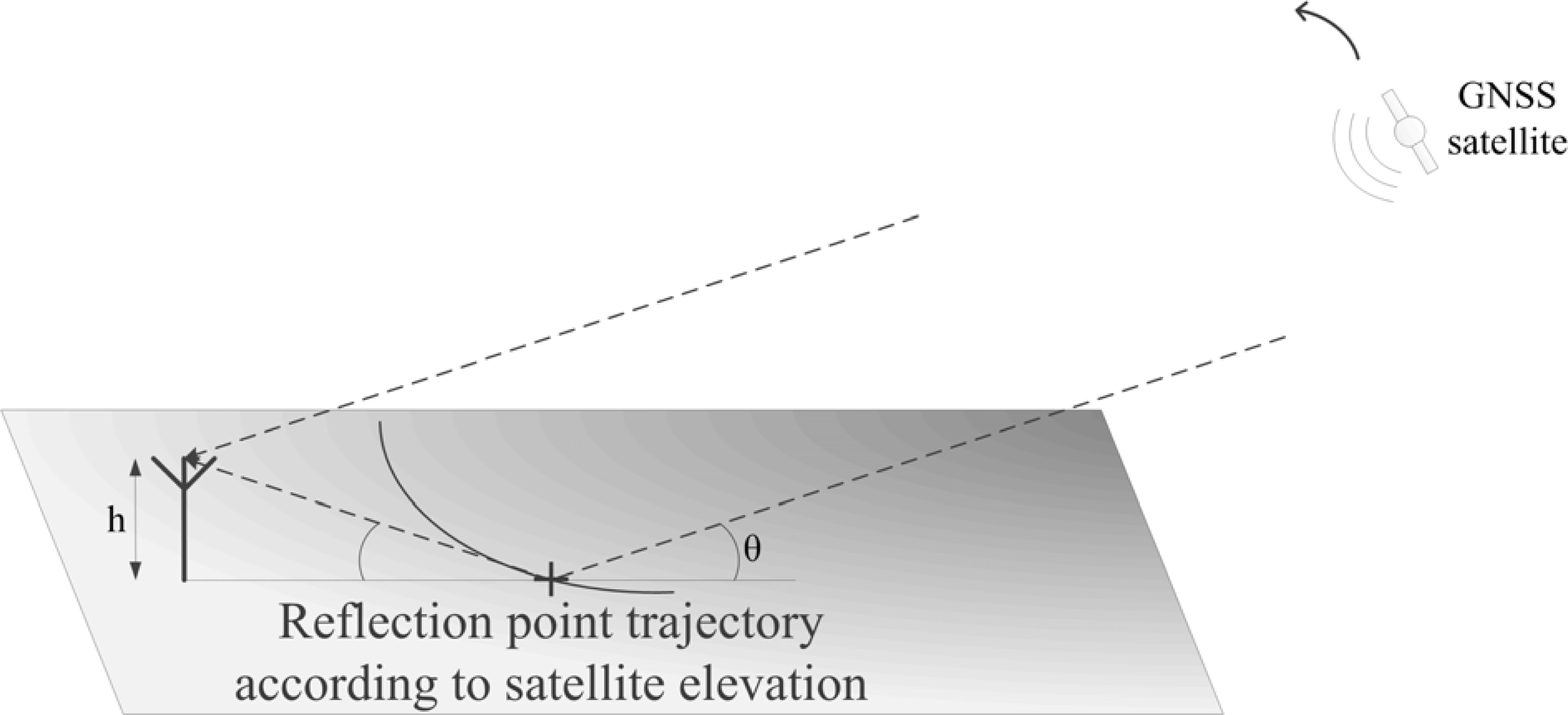
4.1. GNSS-Reflectometry (GNSS-R)

The remote sensing of the Earth using reflected GNSS signals (L-band) such as the American GPS, started at the end of the 1990s. This method, called GNSS-Reflectometry (GNSS-R), uses indirect (i.e., reflected) signals for remote sensing of the Earth’s surface [89]. While observations of the delays of the direct signal allow estimation of the water-vapor in the lower layers of atmosphere and could be conducted with existing instrumentation [90], processing of the reflected signals (normally considered as a noise in a GNSS-receiver) typically requires the construction of new instruments and new signal processing algorithms. Remarkably, relevant geophysical properties of the surface (e.g., soil moisture, water-body roughness and/or salinity retrieval, snow/ice cover determination, etc.) can potentially be retrieved by this approach [17,91,92].

GNSS-R can be implemented on Low Earth Orbit (LEO) satellites [93,94], on aircrafts, or at the ground level [95]. In the former case, the spatial resolution is limited (similarly as with other satellite-based sensing instruments). In the two latter cases, it is possible to cover a relatively large area, considerably wider than with the point-based measurements, yet smaller than for space-based missions, with high resolution, as for regional-scale studies such as those occurring in the alpine environment.

Figure 1 illustrates this concept in a simple local-scale bi-static experiment with a GNSS antenna mounted on a mast above the ground. In this setup, the extra path travelled by the reflected signal can be approximated by 2h sin θ, where h is the height of the antenna phase center above the reflection point and θ the elevation of the satellite. As the navigation satellite is moving across the sky in a Keplerian orbit, the elevation angle and reflectance point is constantly changing on the ground. The power of the reflected signal depends on the surface, which allows the determination of some of its properties. Depending on the roughness of the surface, the reflection can be specular (or coherent) for a smooth surface, or diffuse (non-coherent) for a rough surface [96]. The height of the antenna can also be measured, which means that altimetry measurement can be performed. Considering that almost 20 satellites are potentially observable from any point on the Earth, and this number will almost double in the near future, a map of reflectance properties can be created for the surface around such instrument.

As the extent of current signals from the existing American and Russian satellite systems (i.e., GPS and GLONASS, respectively) is world-wide, there is an enormous potential for exploring this concept and constructing a new type of low-cost remote sensing instrument.

4.1.1. GNSS-R for Soil Moisture Recovery

There are mainly three ways to sense the soil moisture. The first one consists of looking at the reflected signal only, which is the simplest solution but also the one that provides the least information. Such experiments were made in 2002, using a slightly modified commercial GPS receiver airborne [91,97,98]. The reflected signals were obtained from a left-handed circularly polarized (LHCP) antenna at the bottom of the plane. A right-handed circularly polarized (RHCP) antenna was on the top of the plane to receive the direct signals, however the measures were corrupted by multipath and thus not used for normalization purpose. The signal-to-noise ratio (SNR) of the reflected signals were measured and compared to dielectric constant and moisture of the soil. It was shown that the SNR measurements were moderately correlated to the in situ measurements. Still, it was also shown that it was possible to detect field boundaries and that the GPS reflectivity was more correlated to the top 1 cm soil moisture than the soil moisture between 1 and 5 cm. Such an experiment has been done also using Delay-Doppler Maps (DDM), where the power of the reflected signals is computed for different code delay and Doppler frequency [99]. However, it has been shown that only the peak of the DDM was useful [100].

The second option is to receive separately the direct and the reflected signal, and looking at the difference of power [100–102]. This method has the advantage of providing instantaneous measures, however currently it lacks of validation campaign regarding the expected accuracy.

The third possibility is to receive the direct and reflected signal simultaneously through the same antenna. The variation of phase between the two signals causes constructive and destructive interferences that can be exploited to measure the soil moisture. This concept, called Interference Pattern Technique (IPT), has been extensively used by the Universitat Politècnica de Catalunya [17,103,104]. They used a specific receiver for GNSS-R, using vertically and horizontally polarized antennae instead of RHCP only. Thanks to this, they were able to see a notch in the oscillations of the SNR at a certain angle. This is linked to the Brewster angle, which is a particular angle where the reflection coefficient becomes null for vertical polarization [105]. As the Brewster angle depends on the permittivity of the layer, which itself depends on the soil moisture, identifying the position of the reflectance point and hence calculating the Brewster angle provides information about the soil moisture. They have shown promising results over bare and wheat fields, recovering the soil moisture with an error of less than 5%. The drawback of this method is the long recording of signal necessary to extract information (typically few hours).

The interference technique has shown to be applicable also for geodetic antennas as shown by the University of Colorado, which is surprising since the aim of such antennas is to suppress multipath to minimize errors in positioning [92,106,107]. A high correlation between the estimates of the phase of the reflected signals and the height and the soil moisture content at the top centimeter has been shown, however it cannot represent the soil moisture content deeper because of the limited GPS signal penetration.

4.1.2. GNSS-R for Snow Cover Estimation

The IPT has been applied as well to measure the snow height, where multiple notches can be identified. For example, in [108], a very high correlation has been found between the retrieved and true snow height, and it has been shown that the antenna should be as high as possible to obtain better results.

Some important work has also been performed by the University of Colorado in the estimation of snow depth [19,109,110]. The various experiments were performed with geodetic receivers from the EarthScope network. In [110], the authors were able to estimate the snow depth from observations of the modulated SNR to an accuracy of between 9 and 13 cm. However, as stated in [19], this technique only works well when the modulation frequency of the multipath signals can be resolved, i.e., when the area surrounding the GNSS antenna acts as a specular reflector or when the surface is nearly planar, large enough to encompass the first Fresnel zone (FFZ) at lower elevation angles, and free of significant vegetation. This may be a severe limitation for the subalpine region populated with trees, but may not be for the alpine region, in particular in winter when many surface irregularities are filled with snow.

For a ground-based installation, the FFZ for low elevation angles is relatively small (e.g., only a few tens of meters for an antenna 2 m above the ground), and gets larger with the antenna height [19]. The footprint of the antenna will thus depend on the snow height, and will decrease as the snow height increases. For non-horizontal sites, the inclination of the ground should also be taken into account. One possibility suggested in [19] is to observe bare ground in summertime to estimate the vertical distance to the ground. Other possibilities include the use of LIDAR technology or elevation maps. Other parameters that affect this measurement technique are the humidity of the soil (the variation in vertical distance to the ground from this effect is only 2–3 cm) and to a lesser extent the snow density [19].

In the same context, an algorithm has been developed to measure the snow depth based on the geometry-free linear combination, L4, which is the difference of the phases of the L1 and L2 carriers. This algorithm is motivated by the fact that L1 and L2 phases are always recorded by GPS stations, whereas it is not the case for the SNR. However, although the results obtained with this algorithm match those using SNR-based algorithm, the precision is lower [111]. Further studies will include the newer GNSS signals, expecting better precision.

Very few studies have been performed which measure not only the snow depth, but also the snow density, from which the SWE can be obtained. In [112,113], the author proposes an algorithm based on a simple ray model that includes a specular reflected signal along with a direct signal, and includes a nonlinear least squares fitting. The initial results seem promising, but require validation. Indeed, the estimations of the SWE were well within the common values in the region, but there were no in situ field measurements to estimate the validity and accuracy of the results. We note here the similarities between the above method and the radar measurement methods (see Section 3.2.3, meaning that radar and GPR measurement methods are a good reference for the consideration of measurement errors which may be encountered in GNSS-R).

A recent and innovative technique was proposed to characterize the internal layering of dry snow masses [114]. This technique uses the Fourier Transform of the cross-correlation results (also called waveform) and shows a relation between the frequency stripes and the depth of the different snow layers. This technique has been validated by measurement campaigns, however, the current precision is too low for the alpine environment (about 10 m). This is still a preliminary work, and the precision may be improved in the future by improving the model and the use of newer GNSS signals. A summary of the techniques presented in this section is provided in

Table 3. Potential GNSS-R techniques for snow and soil moisture determination.

Technique	Measured Quantity	References	Spatial Range Resolution	Accuracy	Remarks
Extraction of modulation parameters of the SNR	snow depth	[19,109,110]	10’s m	9–13 cm	Use of geodetic RHCP antennas. Limitations for GNSS signals with high chipping rate.
Extraction of modulation parameters of the SNR	soil moisture	[92,106,107]	10’s m	N/A (good agreement)	Use of geodetic RHCP antennas. Limitations for GNSS signals with high chipping rate.
Geometry-free linear combination (L4)	snow depth	[111]	10’s m	cm scale	Technique useful for stations that do not record the SNR.
Simple ray model	snow depth, snow density	[112,113]	10’s m	cm scale	Lack of validation to better estimate the precision of the technique.
Fast Fourier Transform of cross-correlation results (waveforms)	depth of snow layers	[114]	10’s–100’s m	very low (∼10 m)	Results in agreement with real data, despite the low resolution. Measurement performed in Antarctic.
Measure of reflected signals only	soil moisture	[91,97,98]	10’s–100’s m	N/A	Good correlation between GPS reflectivity and soil moisture of the top 1 cm of the soil.
Measure of direct and reflected signals separately	soil moisture	[100–102]	10’s–100’s m	N/A	Promising method, but not yet exploited enough to have quantitative results.
Measure of direct and reflected signals simultaneously (Interference Pattern Technique)	soil moisture	[14,103,104]	10’s m	5% over bare/wheat fields	Use of vertical and horizontal polarization antennas instead of RHCP. Limitations for GNSS signals with high chipping rate.
Measure of direct and reflected signals simultaneously (Interference Pattern Technique)	Snow	[108]	10’s m	N/A (very good agreement)	Use of vertical and horizontal polarization antennas instead of RHCP. Limitations for GNSS signals with high chipping rate.

.

Although the previous investigations of the GNSS-R concept were promising, they are limited in application. Currently, the operation of existing GNSS-R instruments is restricted to “flat surfaces” [115] and cannot yet be applied over complex terrain such as the alpine environment or used to analyze surface properties under vegetation-cover. The reason for this is that the correlation of the reflected signal with the geometrical surroundings needs to be either known a priori (i.e., existence of a flat surface like water-body) or is determined concurrently via long-observation times without moving the GNSS-R instrument. Moreover, a lot of research has been conducted with traditional GPS receivers that use a RHCP antenna. For the reflections, the polarization is affected by the properties of the soil, consequently, to process the signal reflections efficiently, both antenna polarizations should be used, either vertical and horizontal (as in [104]), or LHCP and RHCP. This, however, directly impacts the processing charge, as there are twice as many data to process. Finally, until recently, no substantial research had been conducted over heterogeneous fields or complex landscapes, as this would require consideration of its fine structure to identify the reflection’s specular or diffuse point (s), which is not so easy to determine. Nevertheless, this challenge can potentially be overcome with the advent of new and modernized GNSS signals and signal processing as well as in view of the recent progresses in airborne and terrestrial laser scanning, as further discussed in the next sections.

4.1.3. Future Options for the GNSS-R

As discussed above, the potential of using reflected GNSS signals for studying surface environmental properties has been previously identified, but the exploitation of such signals is still in its infancy. Only a few GNSS-R research instruments have so far been conceived and investigations were usually limited to GPS signals (single frequency L1, or L2C). However, in addition to the USA-owned GPS, the Russian GLONASS constellation of 24 satellites resumed full operation in 2011; the European Union’s Galileo positioning system is in the initial phase of deployment (four In-Orbit Validation satellites are already orbiting); and the People’s Republic of China has announced that it will expand its regional navigation system (named BEIDOU) into a global system (named COMPASS) by 2020. While the signals transmitted by the existing GPS and GLONASS constellations are being modernized with the launch of new satellites, the new Galileo and COMPASS constellations will similarly offer modern signals including wideband modulation, data and pilot channels, longer codes, and transmissions of open service signals over different frequency bands.

Among the properties of these new signals, the first one that will lead to improved signal detection and estimation is a higher power. For example, the future Galileo E1 and GPS L1C signals will have a power 1.5 dB higher than the GPS L1 C/A, and the Galileo E5a and GPS L5 signals will have a power 3.5 and 4.5 dB higher, respectively, which is clearly not negligible. Since the reflected signal is usually weaker than the direct signal, such power increase will proportionally improve the current threshold of detectability.

In the same idea, the second property that will help to improve the detectability threshold is the existence of a pilot channel. Such channel enables the use of very long coherent integrations, while the existing GPS L1 C/A signal, which includes data, requires the use of non-coherent or differentially coherent integrations, which are far less efficient at low SNR [116]. The last major improvements will be the better spatial coverage and the higher number of measures, since more satellites will be visible and each satellite transmits several signals.

By exploiting all these novelties, it is expected that the resolution and the accuracy of the measurement will significantly improve. However, these improvements will come at the price of additional signal processing and research challenges. For example, the chipping rate of the signals at the L5/E5 band is 10 times higher than for the GPS L1 C/A signal, a chip representing a distance of 29.1 m instead of 291 m. This has a direct consequence for some of the proposed GNSS-R techniques, such as those relying on interference due to the carrier only where the direct and reflected codes are assumed aligned [19,104], which is not true anymore even for small extra paths (≤10 m). Therefore, when considering these signals, both the carrier phase and the code alignment have to be considered; otherwise the interference methods discussed previously may provide unreliable results or at least the possible range for the antenna height will be decreased [104].

The current experiments are focused on planar or almost planar terrains, which is an ideal context, but not always representative of the area of interest; typically not applicable in the alpine environment. For such mountainous areas, numerous multiple reflections are likely to happen simultaneously, and not just one. A solution may come from the use of array beamforming, to isolate the different reflections, and apply the traditional algorithms, as well as identify their direction. As the proper calibration of an adaptive antenna array is cumbersome [117,118] and space time adaptive algorithms are very computationally intensive; a possible substitute would be to use a virtual array, such as a synthetic uniform circular array (UCA). Since in this case, a single antenna placed at various pre-defined positions is used (representing the virtual array positions), the amount of data processing is the same as for other conventional temporal frequency processing techniques [119]. Such methods, however, also have an impact on received signal characteristics, such as a high Doppler rate of change (e.g., up to 10 Hz/s instead of 0.65 Hz/s [119]), which implies the design of adapted or new algorithms.

4.2. Wireless Sensor Networks

Wireless sensor networks make it possible to reliably collect sensor data from a large number of point measurements, and are therefore a potential solution for extending the spatial range of point-based measurement techniques. For example, a multi-year field campaign in Val Ferret (VS) in the Swiss Alps uses such a network (Sensorscope) currently consisting of 25 stations distributed over the catchment, measuring relevant meteorological parameters such as rainfall; wind speed and direction; temperature; incoming shortwave radiation and surface temperature of the soil [120]. Soil moisture, soil matric potential, and soil temperatures are also measured at 21 of the stations, using decagon 5TM and ECTM (soil moisture based on dielectric constant) sensors, and MPS1 (matric potential) sensors at 20 and 40 cm below the surface. Nevertheless, Because of the above-mentioned spatial variability of the soil moisture, these point measurements, although numerous and well distributed, can only give a limited picture of basin-wide soil moisture and its distribution. This is also an area where GNSS-R could provide an interesting solution when combined with an existing infrastructure that would provide the necessary data to calibrate the GNSS-R instrument, which in turn would provide measures in-between the in situ infrastructure.

4.3. Airborne Laser Scanning

Elevation models of very fine resolution (at 0.1 m level) and high relative precision (<0.1 m) will be needed for performing GNSS-R analysis over steep or complex terrain, such as in alpine environments. The primary technology that can potentially satisfy such criteria is airborne laser scanning. The performance of commercially available systems utilizing laser scanning technology has increased at an astonishing pace, including a significant reduction of the acquisition time. Surprisingly, rapid development of the accompanying software-tools for automation of data processing, modeling and quality monitoring has not followed. Airborne Laser Scanning (ALS) requires concurrent employment of at least two navigation technologies due to the relatively complicated generation of the laser point-cloud coordinates [121], while the subsequent classification and calculation of digital elevation models (DEM) is even more involved. The algorithmic part of current state-of-the-art research focuses first on the real-time generation of the laser point cloud from moving platforms [122,123]. The second research area develops and implements the classification algorithms (possibly in real-time), which are necessary for the production of digital terrain models (DTM) and for the assessment of scanning geometry, which influences the quality of ALS-derived products [124]. The third research subject treats the obtained mapping accuracy relative to the scanning-target [125] as well to the derived DTM [126].

5. Conclusions

The alpine environment is very complex and challenging to predict, with a very high spatial variability of the soil moisture and fluxes above the surface as well as the snowpack (on a typical 1–10 m scale). Remote observations of soil moisture and snow property determination at scales compatible with the environment’s spatial variability would greatly enhance our ability to understand the physical processes in this type of environment. This would lead to new possibilities, e.g., hydrological modeling, parameterization of atmospheric models, data assimilation in real-time flood and avalanche forecasting systems, etc.

Unfortunately, while different satellite products that would fulfill the large-scale requirements exist, there resolutions are intrinsically not compatible with the small scale and short temporal variations of the alpine environment. On the other hand, while the potential applications of GNSS-R techniques for non-destructive characterization of soil moisture and/or snowpack over large surfaces have been clearly identified, the research is still in its infancy. Indeed, few instruments have been conceived and the investigations were usually limited to simple terrain geometries using GPS signals (single frequency L1 or L2C). Nevertheless, it has been shown that the use of multiple constellation and new signals will have a high positive impact on the resolution and accuracy of GNSS-R measurements. Therefore, we strongly believe that, in the future and as a result of the various research activities that are on-going worldwide, GNSS-R techniques when combined with other techniques such as laser scanning and improved models for the soil parameter extraction will be a very good candidate for filling up the gap on the instrumentation level, thereby opening the use of this technology to applications over more difficult terrain such as the alpine environment.

References

1. Timmons, D.R.; Dylla, A.S. Nitrogen leaching as influenced by nitrogen management and supplemental irrigation level. J. Environ. Qual 1981, 10, 421–426. [Google Scholar]
2. Hergert, G.W. Nitrate leaching through sandy soil as affected by sprinkler irrigation management. J. Environ. Qual 1986, 15, 272–278. [Google Scholar]
3. Trought, M.C.T.; Drew, M.C. The development of waterlogging damage in wheat seedlings (Triticum aestivum L.). Plant Soil 1980, 54, 77–94. [Google Scholar]
4. Lehning, M.; Fierz, C. Assessment of snow transport in avalanche terrain. Cold Reg. Sci. Technol 2008, 51, 240–252. [Google Scholar]
5. Schirmer, M.; Lehning, M.; Schweizer, J. Statistical forecasting of regional avalanche danger using simulated snow-cover data. J. Glaciol 2009, 55, 761–768. [Google Scholar]
6. Grünewald, T.; Schirmer, M.; Mott, R.; Lehning, M. Spatial and temporal variability of snow depth and ablation rates in a small mountain catchment. Cryosphere 2010, 4, 215–225. [Google Scholar]
7. Wirz, V.; Schirmer, M.; Gruber, S.; Lehning, M. Spatio-temporal measurements and analysis of snow depth in a rock face. Cryosphere 2011, 5, 893–905. [Google Scholar] [Green Version]
8. Blanchet, J.; Marty, C.; Lehning, M. Extreme value statistics of snowfall in the Swiss Alpine region. Water Resour. Res 2009, 45, W05424:1–W05424:12. [Google Scholar]
9. Blanchet, J.; Lehning, M. Mapping snow depth return levels: Smooth spatial modeling versus station interpolation. Hydrol. Earth Syst. Sci 2010, 14, 2527–2544. [Google Scholar]
10. Vachaud, G.; Passerat de Silans, A.; Balabanis, P.; Vauclin, M. Temporal stability of spatially measured soil water probability density function. Soil Sci. Soc. Am. J 1985, 49, 822–828. [Google Scholar]
11. Blöschl, G. Scaling in hydrology. Hydrol. Process 2001, 15, 709–711. [Google Scholar]
12. Albertson, J.; Montaldo, N. Temporal dynamics of soil moisture variability: 1. Theoretical basis. Water Resour. Res 2003, 39, 1274:1–1274:14. [Google Scholar]
13. Brocca, L.; Melone, F.; Moramarco, T.; Morbidelli, R. Spatial-temporal variability of soil moisture and its estimation across scales. Water Resour. Res 2010, 46, W02516:1–W02516:14. [Google Scholar]
14. Schmugge, T.; Jackson, T.; McKim, H. Survey of methods for soil moisture determination. Water Resour. Res 1980, 16, 961–979. [Google Scholar]
15. Robinson, D.; Campbell, C.; Hopmans, J.; Hornbuckle, B.; Jones, S.; Knight, R.; Ogden, F.; Selker, J.; Wendroth, O. Soil moisture measurement for ecological and hydrological watershed-scale observatories: A review. Vadose Zone J 2008, 7, 358–389. [Google Scholar]
16. Cardellach, E.; Fabra, F.; Nogués-Correig, O.; Oliveras, S.; Ribó, S.; Rius, A. GNSS-R ground-based and airborne campaigns for ocean, land, ice, and snow techniques: Application to the GOLD-RTR data sets. Radio Sci. 2011, 46, RS0C04:1–RS0C04:16. [Google Scholar]
17. Rodriguez-Alvarez, N.; Bosch-Lluis, X.; Camps, A.; Aguasca, A.; Vall-llossera, M.; Valencia, E.; Ramos-Perez, I.; Park, H. Review of crop growth and soil moisture monitoring from a ground-based instrument implementing the interference pattern GNSS-R technique. Radio Sci. 2011, 46, RS0C03:1–RS0C03:11. [Google Scholar]
18. Egido, A.; Caparrini, M.; Ruffini, G.; Paloscia, S.; Santi, E.; Guerriero, L.; Pierdicca, N.; Floury, N. Global navigation satellite systems reflectometry as a remote sensing tool for agriculture. Remote Sens 2012, 4, 2356–2372. [Google Scholar]
19. Larson, K.M.; Nievinski, F.G. GPS snow sensing: Results from the Earth scope plate boundary observatory. GPS Sol 2013, 1, 41–52. [Google Scholar]
20. Gerrits, A.; Pfister, L.; Savenije, H. Spatial and temporal variability of canopy and forest floor interception in a beech forest. Hydrol. Process 2010, 24, 3011–3025. [Google Scholar]
21. Mott, R.; Schirmer, M.; Bavay, M.; Grünewald, T.; Lehning, M. Understanding snow-transport processes shaping the mountain snow-cover. Cryosphere 2010, 4, 545–559. [Google Scholar]
22. Helbig, N.; Loewe, H.; Mayer, B.; Lehning, M. Explicit validation of a surface shortwave radiation balance model over snow-covered complex terrain. J. Geophys. Res 2010, 115, D18113:1–D18113:12. [Google Scholar]
23. Merz, B.; Plate, E.J. An analysis of the effects of spatial variability of soil and soil moisture on runoff. Water Resour. Res 1997, 33, 2909–2922. [Google Scholar]
24. Rodriguez-Iturbe, I.; Vogel, G.K.; Rigon, R.; Entekhabi, D.; Castelli, F.; Rinaldo, A. On the spatial organization of soil moisture fields. Geophys. Res. Lett 1995, 22, 2757–2760. [Google Scholar]
25. Schirmer, M.; Lehning, M. Persistence in intra-annual snow depth distribution part II: Fractal analysis of snow depth development. Water Resour. Res 2011, 47, W09517:1–W09517:14. [Google Scholar]
26. Clark, M.P.; Hendrikx, J.; Slater, A.G.; Kavetski, D.; Anderson, B.; Cullen, N.J.; Kerr, T.; Hreinsson, E.O.; Woods, R.A. Representing spatial variability of snow water equivalent in hydrologic and land-surface models: A review. Water Resour. Res 2011, 47, W07539:1–W07539:23. [Google Scholar]
27. Mott, R.; Lehning, M. Meteorological modeling of very high resolution wind fields and snow deposition for mountains. J. Hydrometeorol 2010, 11, 934–949. [Google Scholar]
28. Kite, G.W.; Kouwen, N. Watershed modeling using land classifications. Water Resour. Res 1992, 28, 3193–3200. [Google Scholar]
29. Rinaldo, A.; Botter, G.; Bertuzzo, E.; Uccelli, A.; Settin, T.; Marani, M. Transport at basin scales: 1. Theoretical framework. Hydrol. Earth Syst. Sci 2006, 10, 19–29. [Google Scholar]
30. Schweizer, J.; Kronholm, K.; Jamieson, J.B.; Birkeland, K.W. Review of spatial variability of snowpack properties and its importance for avalanche formation. Cold Reg. Sci. Technol 2008, 51, 253–272. [Google Scholar]
31. Egli, L.; Jonas, T.; Meister, R. Comparison of different automatic methods for estimating snow water equivalent. Cold Reg. Sci. Technol 2009, 57, 107–115. [Google Scholar]
32. Mori, Y.; Hopmans, J.; Mortensen, A.; Kluitenberg, G. Multi-functional heat pulse probe for the simultaneous measurement of soil water content, solute concentration, and heat transport parameters. Vadose Zone J 2003, 2, 561–571. [Google Scholar]
33. Steele Dunne, S.C.; Rutten, M.M.; Krzeminska, D.M.; Hausner, M.; Tyler, S.W.; Selker, J.; Bogaard, T.A.; van de Giesen, N.C. Feasibility of soil moisture estimation using passive distributed temperature sensing. Water Resour. Res 2010, 46, W03534:1–W03534:12. [Google Scholar]
34. Rutten, M.M.; Steele-Dunne, S.C.; Judge, J.; van de Giesen, N.C. Understanding heat transfer in the shallow subsurface using temperature observations. Vadose Zone J 2010, 9, 1034–1045. [Google Scholar]
35. Ciocca, F.; Lunati, I.; van de Giesen, N.C.; Parlange, M.B. Heated optical fiber for distributed soil-moisture measurements: A lysimeter experiment. Vadose Zone J 2012, 11, 1–10. [Google Scholar]
36. Alliance Technologies. Available online: http://alliance-technologies.eu/JENOPTIK/Jenoptik/SHM30_Manual_Rev1_1.pdf (accessed on 10 July 2013).
37. Prokop, A.; Schirmer, M.; Rub, M.; Lehning, M.; Stocker, M. A comparison of measurement methods: Terrestrial laser scanning, tachymetry and snow probing for the determination of the spatial snow depth distribution on slopes. Ann. Glaciol 2008, 49, 210–216. [Google Scholar]
38. Hyyppä, J. State of the art in laser scanning. Photogramm. Week 2011, 1, 203–216. [Google Scholar]
39. Schirmer, M.; Wirz, V.; Clifton, A.; Lehning, M. Persistence in intra-annual snow depth distribution part I: Measurements and topographic control. Water Resour. Res 2011, 47, W09516:1–W09516:16. [Google Scholar]
40. Lehning, M.; Grünewald, T.; Schirmer, M. Mountain snow distribution governed by an altitudinal gradient and terrain roughness. Geophys. Res. Lett 2011, 38, L19504:1–L19504:5. [Google Scholar]
41. Sturm, M.; Taras, B.; Liston, G.E.; Derkson, C.; Jonas, T.; Lea, J. Estimating snow water equivalent using snow depth data and climate classes. J. Hydrometeorol 2010, 11, 1380–1394. [Google Scholar]
42. Sundtröm, N.; Kruglyak, A.; Friborg, J. Modeling and simulation of GPR wave propagation through wet snowpacks: Testing the sensitivity of a method for snow water equivalent estimation. Cold Reg. Sci. Technol. 2012, 74–75, 11–20. [Google Scholar]
43. Vallet, J.; Skaloud, J.; Koelbl, O.; Merminod, B. Development of a helicopter-based integrated system for avalanche mapping and hazard management. Int. Arch. Photogramm. Remote Sens. Spat. Inf. Sci 2000, 33, 565–572. [Google Scholar]
44. Etchevers, P.; Martin, E.; Brown, R.; Fierz, C.; Lejeune, Y.; Bazile, E.; Boone, A.; Dai, Y.-J.; Essery, R.; Fernandez, A.; et al. SnowMIP, an Intercomparison of Snow Models: First Results. Proceedings of the International Snow Science Workshop, Pendicton, BC, Canada, 29 September–4 October 2002; 1, pp. 353–360.
45. Etchevers, P.; Martin, E.; Brown, R.; Fierz, C.; Lejeune, Y.; Bazile, E.; Boone, A.; Dai, Y.-J.; Essery, R.; Fernandez, A.; et al. Validation of the energy budget of an alpine snowpack simulated by several snow models (SnowMIP project). Ann. Glaciol 2004, 38, 150–158. [Google Scholar]
46. Lehning, M.; Völksch, I.; Gustafsson, D.; Nguyen, T.A.; Stähli, M.; Zappa, M. ALPINE3D: A detailed model of mountain surface processes and its application to snow hydrology. Hydrol. Process 2006, 20, 2111–2128. [Google Scholar]
47. Bavay, M.; Lehning, M.; Jonas, T.; Löwe, H. Simulations of future snow cover and discharge in alpine headwater catchments. Hydrol. Process 2009, 22, 95–108. [Google Scholar]
48. Lehning, M.; Bartelt, P.; Brown, R.L.; Russi, T.; Stöckli, U.; Zimmerli, M. Snowpack model calculations for avalanche warning based upon a new network of weather and snow stations. Cold Reg. Sci. Technol 1999, 30, 145–157. [Google Scholar]
49. Bell, J. Neutron Probe Practice; Report 19; Institute of Hydrology: Wallingford, UK, 1987; pp. 1–51. [Google Scholar]
50. Zreda, M.; Desilets, D.; Ferré, T.; Scott, R. Measuring soil moisture content non-invasively at intermediate spatial scale using cosmic-ray neutrons. Geophys. Res. Lett 2008, 35, L21402:1–L21402:5. [Google Scholar]
51. Desilets, D.; Zreda, M.; Ferré, T. Nature’s neutron probe: Land surface hydrology at an elusive scale with cosmic rays. Water Resour. Res 2010, 46, W11505:1–W11505:7. [Google Scholar]
52. Topp, G.C.; Davis, J.L.; Annan, A.P. Electromagnetic determination of soil water content: Measurements in coaxial transmission lines. Water Resour. Res 1980, 16, 574–582. [Google Scholar]
53. Kim, D.; Choi, S.; Ryszard, O.; Feyen, J.; Kim, H. Determination of moisture content in a deformable soil using time-domain reflectometry (TDR). Eur. J. Soil Sci 2000, 51, 119–127. [Google Scholar]
54. Robinson, D.A.; Jones, S.B.; Wraith, J.M.; Or, D.; Friedman, S.P. A review of advances in dielectric and electrical conductivity measurement in soils using time domain reflectometry. Vadose Zone J 2003, 2, 444–475. [Google Scholar]
55. Noborio, K. Measurement of soil water content and electrical conductivity by time domain reflectometry: A review. Comput. Electron. Agric 2001, 31, 213–237. [Google Scholar]
56. Heimovaara, T.J. Frequency domain analysis of time domain reflectometry waveforms: 1. Measurement of the complex dielectric permittivity of soils. Water Resour. Res 1994, 30, 189–199. [Google Scholar]
57. Minet, J.; Lambot, S.; Delaide, G.; Huisman, J.A.; Vereecken, H.; Vanclooster, M. A generalized frequency domain reflectometry modeling technique for soil electrical properties determination. Vadose Zone J 2010, 9, 1063–1072. [Google Scholar]
58. Gaskin, G.J.; Miller, J.D. Measurement of soil water content using a simplified impedance measuring technique. J. Agr. Eng. Res 1996, 63, 153–159. [Google Scholar]
59. Wagner, W.; Lemoine, G.; Rott, H. A method for estimating soil moisture from ERS scatterometer and soil data. Remote Sens. Environ 1999, 70, 191–207. [Google Scholar]
60. Bastiaanssen, W.; Menenti, M.; Feddes, R.; Holtslag, A. A remote sensing surface energy balance algorithm for land (SEBAL). 1. Formulation. J. Hydrol. 1999, 212–213, 198–212. [Google Scholar]
61. Kerr, Y.H.; Waldteufel, P.; Wigneron, J.-P.; Delwart, S.; Cabot, F.; Boutin, J.; Escorihuela, M.-J.; Font, J.; Reul, N.; Gruhier, C.; et al. The SMOS mission: New tool for monitoring key elements of the global water cycle. Proc. IEEE 2010, 98, 666–687. [Google Scholar]
62. Camps, A.; Font, J.; Corbella, I.; Vall-Llossera, M.; Portabella, M.; Ballabrera-Poy, J.; González, V.; Piles, M.; Aguasca, A.; Acevo, R.; et al. Review of the CALIMAS team contributions to European space agency’s soil moisture and ocean salinity mission calibration and validation. Remote Sens 2012, 4, 1272–1309. [Google Scholar]
63. Entekhabi, D.; Njoku, E.G.; O’Neill, P.E.; Kellogg, K.H.; Crow, W.T.; Edelstein, W.N.; Entin, J.K.; Goodman, S.D.; Jackson, T.J.; Johnson, J.; et al. The soil moisture active passive (SMAP) mission. Proc. IEEE 2010, 98, 704–716. [Google Scholar]
64. Winsemius, H.; Savenije, H.; van de Giesen, N.; van den Hurk, B.; Zapreeva, E.; Klees, R. Assessment of gravity recovery and climate experiment (grace) temporal signature over the upper zambezi. Water Resour. Res 2006, 42, W12201:1–W12201:8. [Google Scholar]
65. Frei, A.; Tedesco, M.; Lee, S.; Foster, J.; Hall, D.K.; Kelly, R.; Robinson, D.A. A review of global satellite-derived snow products. Adv. Space Res 2012, 50, 1007–1029. [Google Scholar]
66. Nolin, A. Recent advances in remote sensing of seasonal snow. J. Glaciol 2010, 56, 1141–1150. [Google Scholar]
67. König, M.; Winther, J.G.; Isaksson, E. Measuring snow and glacier ice properties from satellite. Rev. Geophys 2001, 39, 1–28. [Google Scholar]
68. Foppa, N.; Stoffel, A.; Meister, R. Synergy of in situ and space borne observation for snow depth mapping in the Swiss Alps. Int. J. Appl. Earth Obs. Geoinf 2007, 9, 294–310. [Google Scholar]
69. Molotch, N.P.; Margulis, S.A. Estimating the distribution of snow water equivalent using remotely sensed snow cover data and a spatially distributed snowmelt model: a multi-resolution, multi-sensor comparison. Adv. Water Resour 2008, 31, 1503–1514. [Google Scholar]
70. Durand, M.; Molotch, N.P.; Margulis, S.A. Merging complementary remote sensing datasets in the context of snow water equivalent reconstruction. Remote Sens. Environ 2008, 112, 1212–1225. [Google Scholar]
71. Thirel, G.; Salamon, P.; Burek, P.; Kalas, M. Assimilation of MODIS snow cover area data in a distributed hydrological model. Hydrol. Earth Syst. Sci 2011, 8, 1329–1364. [Google Scholar]
72. Hall, D.K.; Riggs, G.A.; Salomonson, V.V.; DiGirolamo, N.; Bayr, K.J. MODIS snow-cover products. Remote Sens. Environ 2002, 83, 181–194. [Google Scholar]
73. Guneriussen, T.; Hogda, K.A.; Johnson, H.; Lauknes, I. InSAR for estimation of changes in snow water equivalent of dry snow. IEEE Trans. Geosci. Remote Sens 2001, 39, 2101–2108. [Google Scholar]
74. Song, Y.S.; Sohn, H.G.; Park, C.H. Efficient water area classification using Radarsat-1 SAR imagery in a high relief mountainous environment. Photogramm. Eng. Remote Sensing 2007, 73, 285–296. [Google Scholar]
75. Chang, A.T.C.; Foster, J.L.; Hall, D.K. Nimbus-7 SMMR derived global snow cover parameters. Ann. Glaciol 1987, 9, 39–44. [Google Scholar]
76. Tedesco, M.; Narvekar, P.S. Assessment of the NASA AMSR-E SWE product. IEEE J. Sel. Top. Appl. Earth Obs. Remote Sens 2010, 3, 141–159. [Google Scholar]
77. Clifford, D. Global estimates of snow water equivalent from passive microwave instruments: History, challenges and future developments. Int. J. Remote Sens 2010, 31, 3707–3726. [Google Scholar]
78. Kelly, R.E.J.; Chang, A.T.C.; Tsang, L.; Foster, J.L. Development of a prototype AMSR-E global snow area and depth algorithm. IEEE Trans. Geosci. Remote Sens 2003, 41, 230–242. [Google Scholar]
79. Kelly, R.E.J. The AMSR-E snow depth algorithm: Description and initial results. J. Remote Sens. Soc. Jpn 2009, 29, 307–317. [Google Scholar]
80. Walker, A.E.; Goodison, B.E. Discrimination of a wet snowcover using passive microwave satellite data. Ann. Glaciol 1993, 17, 307–311. [Google Scholar]
81. Foster, J.L.; Sun, C.; Walker, J.P.; Kelly, R.; Chang, A.; Dong, J.; Powell, H. Quantifying the uncertainty in passive microwave snow water equivalent observations. Remote Sens. Environ 2005, 94, 187–203. [Google Scholar]
82. Matzler, C. Passive microwave signatures of landscapes in winter. Meteorol. Atmos. Phys 1994, 54, 241–260. [Google Scholar]
83. Hancock, S.; Baxter, R.; Evans, J.; Huntley, B. Evaluating global snow water equivalent products for testing land surface models. Remote Sens. Environ 2013, 128, 107–117. [Google Scholar] [Green Version]
84. Grasty, R. Direct snow-water equivalent measurement by air-borne gamma-ray spectrometry. J. Hydrol 1982, 55, 213–235. [Google Scholar]
85. Martin, J.-P.; Houdayer, A.; Lebel, C.; Choquette, Y.; Lavigne, P.; Ducharme, P. An Unattended Gamma Monitor for the Determination of Snow Water Equivalent (SWE) Using the Natural Ground Gamma radiation. Proceedings of IEEE Nuclear Science Symposium (NSS), Dresden, Germany, 19–25 October 2008; pp. 983–988.
86. Reginato, R.J.; van Bavel, C.H.M. Soil water measurement with gamma attenuation. Soil Sci. Soc. Am. J 1964, 28, 721–724. [Google Scholar]
87. Gardner, W.H.; Campbell, G.S.; Calissendorff, C. Systematic and random errors in dual gamma energy soil bulk density and water content measurements. Soil Sci. Soc. Am. J 1972, 36, 393–398. [Google Scholar]
88. Davidson, J.M.; Biggar, J.W.; Nielsen, D.R. Gamma-radiation attenuation for measuring bulk density and transient water flow in porous materials. J. Geophys. Res 1963, 68, 4777–4783. [Google Scholar]
89. Martin-Neira, M. A passive reflectometry and interferometry system (PARIS): Application to ocean altimetry. ESA J 1993, 17, 331–355. [Google Scholar]
90. Troller, M.; Geiger, A.; Kahle, H.-G. Swiss Geodetic Commission, Determination of the Spatial Distribution of Water Vapor above Switzerland Using GPS Tomography. Proceedings of XXIV International Union of Geodesy and Geophysics (IUGG) General Assembly, Perugia, Italy, 2–13 July 2007; pp. 137–138.
91. Katzberg, S.J.; Torres, O.; Grant, M.S.; Masters, D. Utilizing calibrated GPS reflected signals to estimate soil reflectivity and dielectric constant: Results from SMEX02. Remote Sens. Environ 2006, 100, 17–28. [Google Scholar]
92. Larson, K.M.; Braun, J.J.; Small, E.E.; Zavorotny, V.U.; Gutmann, E.; Bilich, A.L. GPS multipath and its relation to near-surface soil moisture content. IEEE J. Sel. Top. Appl. Earth Obs. Remote Sens 2010, 3, 91–99. [Google Scholar]
93. Gleason, S. Remote Sensing of Ocean, Ice and Land Surfaces Using Bistatically Scattered GNSS Signals from Low Earth Orbit. 2006. [Google Scholar]
94. Gleason, S. Towards sea ice remote sensing with space detected GPS signals: Demonstration of technical feasibility and initial consistency check using low resolution sea ice information. Remote Sens 2010, 2, 2017–2039. [Google Scholar]
95. Gleason, S.; Gebre-Egziabher, D. GNSS Applications and Methods; Artech House: Norwood, MA, USA, 2009. [Google Scholar]
96. Pierdicca, N.; Guerriero, L.; Brogioni, M.; Egido, A. On the Coherent and Non Coherent Components of Bare and Vegetated Terrain Bistatic Scattering: Modelling the GNSS-R Signal over Land. Proceedings of IEEE International Geosciences and Remote Sensing Symposium (IGARSS’12), Munich, Germany, 22–27 July 2012; pp. 3407–3410.
97. Masters, D.; Axelrad, P.; Katzberg, S. Initial results of land-reflected GPS bistatic radar measurements in SMEX02. Remote Sens. Environ 2004, 92, 507–520. [Google Scholar]
98. Grant, M.S.; Acton, S.T.; Katzberg, S.J. Terrain moisture classification using GPS surface-reflected signals. IEEE Geosci. Remote Sens. Lett 2007, 4, 41–45. [Google Scholar]
99. Valencia, E.; Camps, A.; Vall-llossera, M.; Monerris, A.; Bosch-Lluis, X.; Rodriguez-Alvarez, N.; Ramos-Perez, I.; Marchan-Hernandez, J.F.; Martinez-Fernandez, J.; Sanchez-Martin, N.; et al. GNSS-R Delay-Doppler Maps over Land: Preliminary Results of the GRAJO Field Experiment. Proceedings of IEEE International Geosciences and Remote Sensing Symposium (IGARSS’10), Honolulu, HI, USA, 25–30 July 2010; pp. 3805–3808.
100. Camps, A.; Forte, G.; Ramos, I.; Alonso, A.; Martinez, P.; Crespo, L.; Alcayde, A. Recent Advances in Land Monitoring Using GNSS-R Techniques. Proceedings of Workshop Reflectometry Using GNSS and Other Signals of Opportunity (GNSS+R), West Lafayette, IN, USA, 10–11 October 2012; pp. 1–4.
101. Li, Q.; Reboul, S.; Boutoille, S.; Choquel, J.-B.; Benjelloun, M.; Gardel, A. Beach soil moisture measurement with a land reflected GPS bistatic radar technique. Proceedings of New Trends for Environmental Monitoring Using Passive Systems, French Riviera, 14–17 October 2008; pp. 1–6.
102. Bourkane, A.; Reboul, S.; Azmani, M.; Choquel, J.-B.; Amami, B.; Benjelloun, M. C/N0 Inversion for Soil Moisture Estimation Using Land-Reflected Bi-Static Radar Measurements. Proceedings of Workshop on Reflectometry Using GNSS and Other Signals of Opportunity (GNSS+R), West Lafayette, IN, USA, 10–11 October 2012; pp. 1–5.
103. Rodriguez-Alvarez, N.; Bosch-Lluis, X.; Camps, A.; Vall-Llossera, M.; Valencia, E.; Marchan, J.F.; Ramos-Perez, I. Soil moisture retrieval using GNSS-R techniques: Experimental results over a bare soil field. IEEE Trans. Geosci. Remote Sens 2009, 47, 3616–3624. [Google Scholar]
104. Rodriguez-Alvarez, N.; Camps, A.; Vall-llossera, M.; Bosch-Lluis, X.; Monerris, A.; Ramos-Perez, I.; Valencia, E.; Marchan-Hernandez, J.F.; Martinez-Fernandez, J.; Baroncini-Turricchia, G.; et al. Land geophysical parameters retrieval using the interference pattern GNSS-R Technique. IEEE Trans. Geosci. Remote Sens 2011, 49, 71–84. [Google Scholar]
105. Balanis, C.A. Advanced Engineering Electromagnetics; John Wiley & Sons: New York, NY, USA, 2009. [Google Scholar]
106. Larson, K.M.; Small, E.E.; Gutmann, E.; Bilich, A.; Axelrad, P.; Braun, J. Using GPS multipath to measure soil moisture fluctuations: Initial results. GPS Sol 2008, 12, 173–177. [Google Scholar]
107. Larson, K.M.; Small, E.E.; Gutmann, E.; Bilich, A.; Axelrad, P.; Braun, J.; Zavorotny, V.U. Use of GPS receivers as a soil moisture network for water cycle studies. Geophys. Res. Lett 2008, 32, L24405:1–L24405:5. [Google Scholar]
108. Rodriguez-Alvarez, N.; Aguasca, A.; Valencia, E.; Bosch-Lluis, X.; Camps, A.; Ramos-Perez, I.; Park, H.; Vall-llossera, M. Snow thickness monitoring using GNSS measurements. IEEE Geosci. Remote Sens. Lett 2012, 9, 1109–1113. [Google Scholar]
109. Larson, K.M.; Gutmann, E.; Zavorotny, V.U.; Braun, J.; Williams, M.W. Can we measure snow depth with GPS receivers? Geophys. Res. Lett 2009, 36, L17502:1–L17502:5. [Google Scholar]
110. Gutmann, E.D.; Larson, K.M.; Williams, M.W.; Nievinski, F.G.; Zavorotny, V. Snow measurement by GPS interferometric reflectometry: An evaluation at Niwot Ridge, Colorado. Hydrol. Process 2011, 26, 2951–2961. [Google Scholar]
111. Ozeki, M.; Heki, K. GPS snow depth meter with geometry-free linear combinations of carrier phases. J. Geod 2012, 86, 209–219. [Google Scholar]
112. Jacobson, M.D. Dielectric-covered ground reflectors in GPS multipath reception—Theory and measurement. IEEE Geosci. Remote Sens. Lett 2008, 5, 396–399. [Google Scholar]
113. Jacobson, M.D. Inferring snow water equivalent for a snow-covered ground reflector using GPS multipath signals. Remote Sens 2010, 2, 2426–2441. [Google Scholar]
114. Fabra, F.; Cardellach, E.; Nogues-Correig, O.; Oliveras, S.; Ribo, S.; Rius, A.; Macelloni, G.; Pettinato, S.; D’Addio, S. An Empirical Approach towards Characterization of Dry Snow Layers Using GNSS-R. Proceedings of IEEE International Geosciences and Remote Sensing Symposium (IGARSS’11), Vancouver, BC, Canada, 24–29 July 2011; pp. 4379–4382.
115. Yang, D.; Zhou, Y.; Wang, Y. Remote sensing with reflected signals. Inside GNSS 2009, 6, 40–45. [Google Scholar]
116. Borio, D.; O’Driscoll, C.; Lachapelle, G. Coherent, noncoherent, and differentially coherent combining techniques for acquisition of new composite GNSS signals. IEEE Trans. Aerosp. Electron. Syst 2009, 45, 1227–1240. [Google Scholar]
117. Church, C.M.; O’Brien, A.J.; Gupta, I.J. A novel method to measure array manifolds of GNSS adaptive antennas. J. Inst. Navig 2011, 59, 345–356. [Google Scholar]
118. Keshvadi, M.H.; Broumandan, A.; Lachapelle, G. Analysis of GNSS Beamforming and Angle of Arrival Estimation in Multipath Environments. Proceedings of the Institute of Navigation’s 2011 International Technical Meeting (ION ITM), San Diego, CA, USA, 24–26 January 2011; pp. 427–435.
119. Lin, T.; Broumandan, A.; Nielsen, J.; O’Driscoll, C.; Lachapelle, G. Robust Beamforming for GNSS Synthetic Antenna Arrays. Proceedings of the 22nd International Technical Meeting of the Satellite Division of the Institute of Navigation (ION GNSS 2009), Savannah, GA, USA, 22–25 September 2009; pp. 387–401.
120. Simoni, S.; Padoan, S.; Nadeau, D.; Diebold, M.; Porporato, A.; Barrenetxea, G.; Ingelrest, F.; Vetterli, M.; Parlange, M. Hydrologic response of an alpine watershed: Application of a meteorological wireless sensor network to understand streamflow generation. Water Resour. Res 2001, 47, W10524:1–W10524:16. [Google Scholar]
121. Glennie, C. Rigorous 3D error analysis of kinematic scanning LIDAR systems. J. Appl. Geod 2007, 1, 147–157. [Google Scholar]
122. Skaloud, J.; Schaer, P.; Stebler, Y.; Tomé, P. Real-time registration of airborne laser data with sub-decimeter accuracy. ISPRS J. Photogramm 2010, 65, 208–217. [Google Scholar]
123. Skaloud, J.; Schaer, P. Optimizing computational performance for real-time mapping with airborne laser scanning. Int. Arch. Photogramm. Remote Sens. Spat. Inf. Sci 2010, 38, 1–5. [Google Scholar]
124. Schaer, P.; Skaloud, J.; Landtwig, S.; Legat, K. Accuracy estimation for laser point cloud including scanning geometry. Int. Arch. Photogramm. Remote Sens. Spat. Inf. Sci 2007, 36, 1–8. [Google Scholar]
125. Schaer, P.; Skaloud, J.; Tomé, P. Towards in-flight quality assessment of airborne laser scanning. Int. Arch. Photogramm. Remote Sens. Spat. Inf. Sci 2008, 37, 1–6. [Google Scholar]
126. Skaloud, J.; Schaer, P. Automated assessment of digital terrain models derived from airborne laser scanning. Photogramm. Fernerkund. Geoinf 2012, 2, 105–114. [Google Scholar]
Figure 1. Example of a local-scale static GNSS-R experiment.
Remotesensing 05 03516f1