Abstract
We evaluated the precision of land surface temperature (LST) operationally retrieved from the Korean multipurpose geostationary satellite, Communication, Ocean and Meteorological Satellite (COMS). The split-window (SW)-type retrieval algorithm was developed through radiative transfer model simulations under various atmospheric profiles, satellite zenith angles, surface emissivity values and surface lapse rate conditions using Moderate Resolution Atmospheric Transmission version 4 (MODTRAN4). The estimation capabilities of the COMS SW (CSW) LST algorithm were evaluated for various impacting factors, and the retrieval accuracy of COMS LST data was evaluated with collocated Moderate Resolution Imaging Spectroradiometer (MODIS) LST data. The surface emissivity values for two SW channels were generated using a vegetation cover method. The CSW algorithm estimated the LST distribution reasonably well (averaged bias = 0.00 K, Root Mean Square Error (RMSE) = 1.41 K, correlation coefficient = 0.99); however, the estimation capabilities of the CSW algorithm were significantly impacted by large brightness temperature differences and surface lapse rates. The CSW algorithm reproduced spatiotemporal variations of LST comparing well to MODIS LST data, irrespective of what month or time of day the data were collected from. The one-year evaluation results with MODIS LST data showed that the annual mean bias, RMSE and correlation coefficient for the CSW algorithm were −1.009 K, 2.613 K and 0.988, respectively.
1. Introduction
Land surface temperature (LST) is a key variable used in a wide range of applications, such as in the monitoring of the surface radiation budget, climate change, the hydrological cycle and ecosystems [1–4]. In spite of the recognized importance of LST, in situ measurements of LST over continents are not yet adequate for resolving diurnal cycles or for analyzing synoptic, seasonal and interannual variability, because of strong spatiotemporal variations in the data and difficulties in accurate measurements. Remote sensing instruments onboard satellites working in the thermal infrared channels are the only available operational systems capable of collecting cost-effective LST data at spatial and temporal resolutions that are appropriate for various applications [5–9].
After it was proven that the LST data could theoretically be retrieved using a split-window (SW) method, many attempts were made to compute LST from satellite data, especially for data collected by polar orbiting satellites (e.g., National Oceanic and Atmospheric Administration (NOAA) / Advanced Very High Resolution Radiometer (AVHRR), Terra/Moderate Resolution Imaging Spectroradiometer (MODIS) and Landsat / Thematic Mapper (TM)) [1,2,10–12]. Similar to the retrieval of sea-surface temperature (SST), LST estimations from satellite remote sensing data are typically obtained from one or more thermal infrared channels located in the atmospheric window region of 8–13 μm. Among the various types of LST retrieval methods available, the SW technique is one of the most widely used methods for retrieving LST from both polar orbiting and geostationary satellite data [1–3,6,10]. This method is based on the assumption that the surface emissivities of SW channels are known a priori [6,13]. However, the lack of high-quality surface emissivity data with sufficient spatiotemporal resolution is a major obstacle for retrieving LST from the satellite data [14–19].
Recently, two databases containing surface emissivity information were developed by the University of California, Santa Barbara [20], and Johns Hopkins University (JHU) [21]. In addition, various background data (land cover, vegetation index, etc.) and methods for estimating surface emissivity have been significantly improved [14,22–24]. As a result, LST data with global coverage, which includes LST data from polar orbiting satellites (e.g., Terra/MODIS [25]) and geostationary satellites (e.g., Meteosat Second Generation (MSG)/Spinning Enhanced Visible and Infra-Red Imager (SEVIRI) [26]) can now be operationally retrieved and serviced to different users [6,27–30].
Given that the Asian continent is not only the largest continent in the world, but is also a strong modulator of the East Asian monsoon system, it is true that relatively few work for the LST retrieval has been done on this region compared to the European and American regions [2,6,18,30]. Hong et al. [31] developed an SW-type LST algorithm using Multi-functional Transport Satellite-1 Replacement (MTSAT-1R) data and investigated the sensitivity of the LST algorithm to various impacting factors, such as the difference between LST and air temperature, emissivity values, satellite zenith angles (SZAs) and brightness temperature differences (BTDs). Furthermore, Tang et al. [32] retrieved LST data using a generalized SW algorithm from China’s geostationary meteorological satellite (Feng Yun-2C (FY-2C)) data. The Korea Meteorological Administration (KMA) successfully launched the first Korean multipurpose geostationary satellite, Communication, Ocean and Meteorological Satellite (COMS) on 27 June 2010. COMS is located above the Equator at longitude 128°E and is equipped with a meteorological imager comprising one visible channel (1 km) and four infrared channels (4 km). A detailed description for the COMS meteorological imager is given in Table 1. After an intensive operational test of COMS, full operation of COMS began on 1 April 2011. KMA also developed a COMS meteorological data-processing system (CMDPS) for the successful operation and efficient use of COMS data [33]. Various meteorological variables, such as cloud cover, aerosol optical depth, SST and LST are being derived automatically by CMDPS from COMS level-1b data and auxiliary data. Hong et al. [34] improved the LST retrieval algorithm from COMS data based on the day and night conditions. However, the evaluation results with Moderate Resolution Imaging Spectroradiometer (MODIS) LST data showed that it has a systematic positive bias caused by prescription errors in the emissivity [35]. Therefore, we redeveloped the LST retrieval algorithm in this study.

Table 1.
Summary of Communication, Ocean and Meteorological Satellite (COMS) meteorological imager used in this study.
The objective of this study is to introduce the LST retrieval algorithm being operated by KMA’s National Meteorological Satellite Center as part of CMDPS. Section 2 describes how the LST retrieval algorithm was developed from two of the COMS thermal channel datasets using simulated data with Moderate Resolution Atmospheric Transmission version 4 (MODTRAN4) over a wide range of surface and atmospheric conditions. Section 3 describes the estimation process used for generating surface emissivity data for the COMS two thermal channels. Section 4 gives an example of LST data retrieved from the COMS data and discusses the validity of these results by comparing them to MODIS LST data. A summary of this study is given in Section 5.
2. Development of LST Retrieval Algorithm
In general, numerous ground truth LST data are needed to develop an LST retrieval algorithm using statistical regression methods. However, unlike the SST, the available match-up data (i.e., ground-level observational data) for LST over the COMS observing region (Figure 1) are severely limited. Hence, we generated pseudo match-up data through radiative transfer model simulations using MODTRAN4 over a wide range of atmospheric and surface conditions. In this paper, MODTRAN4 [36] has been used, because it represents the state-of-the-art in realistic computing of absorption and scattering in the terrestrial atmosphere at high spectral resolution (1 cm−1) over the various infrared spectral ranges, providing accurate simulations of atmospheric radiative transfer [37–39]. Furthermore, the model was based on the angular dependence of the detected radiance, similar to what has been done in previous studies [2,31,32,40]. We assumed that the sky was completely clear and that the main factors affecting the accuracy of the retrieved LST data using the SW method were atmospheric profiles of temperature and water vapor, surface emissivity, SZA and lapse rate at the surface layer.
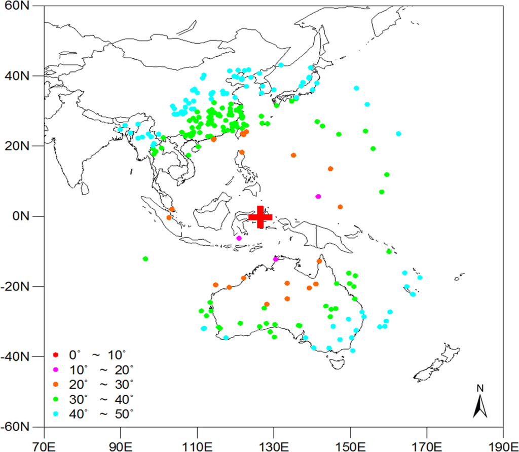
Figure 1.
Spatial distribution of Thermodynamic Initial Guess Retrieval (TIGR) data used in this study. The nadir position of COMS is represented by “
 .
.
.
The radiative transfer simulations were designed to include all of the impacting factors (Table 2). To account for atmospheric effects, we used the latest version of the Thermodynamic Initial Guess Retrieval (TIGR) database, version TIGR2000_6CORPS, which was constructed by the Laboratoire de Météorologie Dynamique [41]. Of the total TIGR database, only 359 stations were selected for use in this study. These stations are geographically located within 50° of SZA from the COMS nadir position (see Figure 1). In this study, SZA was calculated for each TIGR data point. In general, the diurnal variations of LST are much greater than those for air temperature (Ta), especially in dry regions, such as desert and semidesert regions. To account for the large diurnal variation of LST, it was set to vary from (Ta − 6) K to (Ta + 16) K in progressive increments equivalent to 2 K. Here, Ta represents the air temperature of the lowest layer in the TIGR data. The surface emissivity for the infrared radiation channel IR1 was set to vary from 0.9478 to 0.9968 in progressive increments of 0.0049, and the emissivity difference between IR1 and IR2 channels was set to vary from −0.012 to 0.012 in progressive increments of 0.004. The conditions used in this study are similar to Sobrino and Romaguera [40] and Tang et al. [32]. As a result, the number of total simulations amounted to 359 (profiles and SZAs) × 12 (surface lapse rates) × 11 (emissivity values) × 7 (emissivity differences) = 331,716.
Table 2.
Atmospheric, surface and sensor-target conditions used in radiative transfer model simulations. SZA, satellite zenith angles.
The brightness temperatures of the two SW channels were produced using the averaged radiances generated through the radiative transfer model simulations and the COMS spectral response function via an inverse Planck equation (Figure 2). The spectral response functions of COMS IR1 and IR2 are slightly different from those of the Spinning Enhanced Visible and Infra-Red Imager (SEVIRI) instrument onboard the Meteosat Second Generation 2 (MSG2) satellite. In this study, we developed an SW-type LST retrieval algorithm, because the accuracy and efficiency of SW-type LST algorithms are well known [2,3,16,31,32,40]. Various types of linearized SW algorithms have been developed based on the differential absorption in two adjacent split-window channels (10–12.5 μm) linearizing the radiative transfer equation (e.g., [1–3,6,10]). In general, these algorithms express the LST as a simple linear combination of the impacting factors, such as brightness, temperature difference, SZA and emissivity [1–3,6,10,16]. However, the linearized SW algorithm results in large errors in LST retrieval under wet and hot atmospheric conditions [42,43]. To improve the accuracy of LST retrieval, various types of non-linear SW algorithms have been developed [42–44]. We included a non-linear term (ΔT2) for water vapor to account for its non-linear impacts as in Sobrino and Raissouni [43] and Sun and Pinker [44]. This approach is different from other approaches that separate the retrieval equations according to the atmospheric water vapor content [2,32]. The equation used for this study was:
where TIR1 is the brightness temperature of IR1, θ is the SZA of COMS, ΔT = TIR1 − TIR2,
and Δε = εIR1 − εIR2. The coefficients from a to g in the CSW algorithm were determined with the simulated brightness temperature data and the prescribed LST data using the statistical regression method, as shown in Equation (2):
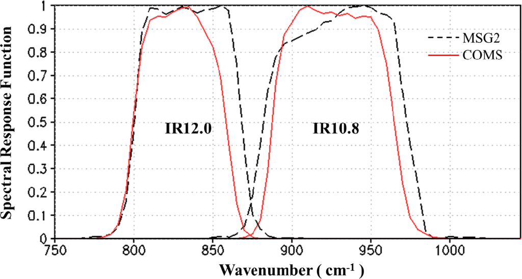
Figure 2.
Comparison of COMS IR1 and IR2 spectral response functions with those from Spinning Enhanced Visible and Infra-Red Imager (SEVIRI) on Meteosat Second Generation 2 (MSG2).
Figure 3 shows a histogram of bias and a scatter plot of the prescribed and estimated LSTs by the COMS Split-Window (CSW) retrieval algorithm for the full range of simulation conditions. In general, the CSW retrieval algorithm slightly overestimated the LST compared to the prescribed LST, except in situations where the LST was between 300 K and 320 K. Although the average estimation capabilities of the CSW retrieval algorithm were very high (averaged bias = 0.00 K, RMSE = 1.41 K, correlation coefficient = 0.99), the bias covered a wide spectrum ranging from −4 K to +4 K. These results suggest that the current CSW retrieval algorithm can significantly either overestimate or underestimate the LST under certain conditions.
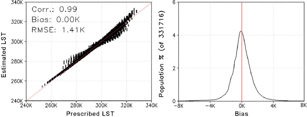
Figure 3.
Scatter plot (left) of prescribed land surface temperature (LST) and estimated LST using the database simulated by Moderate Resolution Atmospheric Transmission version 4 (MODTRAN4) for the full range of conditions; histogram (right) of the difference between the prescribed LST and estimated LST.
The estimation capabilities of the CSW algorithm varied according to the surface lapse rate conditions (i.e., the diurnal variation of the difference between LST and air temperature). These data are shown in Figure 4. While the estimation capabilities of the CSW algorithm were clearly impacted by the lapse rate conditions, the algorithm produced more accurate estimations (i.e., high correlation, small bias and RMSE) under weak lapse rate conditions. However, the CSW algorithm had less estimation capabilities (i.e., low correlation, large bias and RMSE) when there were strong lapse rate conditions, especially under strong inversion and superadiabatic conditions.
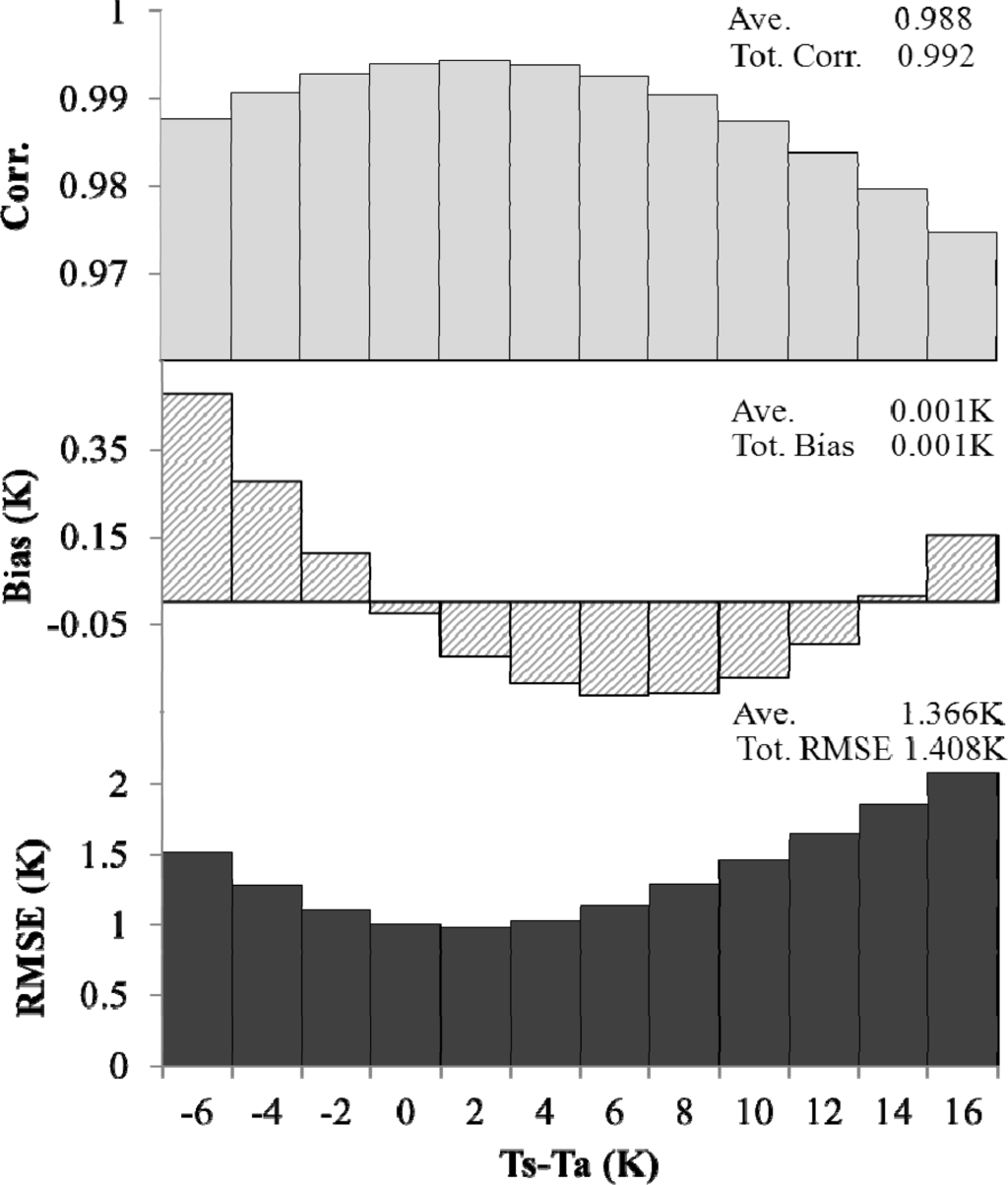
Figure 4.
Estimation skills of COMS Split-Window LST retrieval algorithm according to the difference between LST and air temperature.
Figure 5 shows the RMSE distribution of the CSW retrieval algorithm according to various impacting factors. SZA, brightness temperature difference (BTD) and emissivity difference also impacted the estimation capabilities of the CSW algorithm in addition to the surface lapse rate (Figure 5a,c–f). A negative and a positive BTD exaggerated the RMSE of the CSW algorithm under strong inversion and superadiabatic conditions, respectively (Figure 5d). A negative BTD can be caused by negative emissivity differences and aerosols [45]. The impacts of the emissivity differences on the estimated LST were very similar to those of the BTD differences, but the intensity of the impacts was less significant (Figure 5e). The impacts of emissivity differences and BTD indicate that the quality of LST data retrieved by the CSW algorithm over regions with large diurnal variations in LST (e.g., desert or semidesert regions) can be significantly deteriorated at certain times of the day, in particular, during early morning hours and at noon. Furthermore, the impacts of SZA were proportional to the SZA and more significant under strong inversion and superadiabatic conditions (Figure 5c). Figure 5 indicates that the quality of the retrieved LST by this algorithm may be poor when there are large lapse rates, SZAs, BTDs and emissivity differences present. However, the impacts of mean emissivity and differences between two thermal channel emissivities on the correlation were relatively weak (data not shown). In general, the estimation capabilities of the CSW algorithm worked reasonably well for the values varying from −1 to +4 K (BTD), −2 to +8 K (LST − Ta), and <50° (SZA).
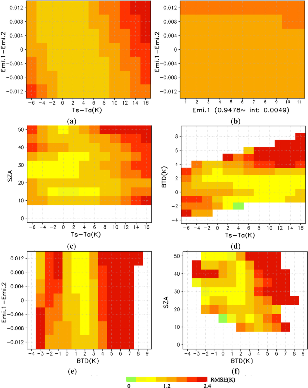
Figure 5.
Distribution of RMSE for COMS Split-Window LST algorithm according to different impacting factors: (a) surface lapse rate and emissivity difference; (b) emissivity of infrared-1 and emissivity difference; (c) surface lapse rate and satellite zenith angle; (d) surface lapse rate and brightness temperature difference; (e) brightness temperature difference and emissivity difference; (f) brightness temperature difference and satellite zenith angle.
3. Estimation of Surface Emissivity
Most types of SW LST algorithms are based on the assumption that the surface emissivity of the two SW channels is known a priori. In this study, the vegetation cover method (VCM) presented by Valor and Caselles [14] was used to generate surface emissivity data for the two SW channels. This method is based on the assumption that each pixel is composed of soil and vegetation [10,46]. The spatiotemporal variations of surface emissivity were generated by the VCM method through the use of a spatially varying land cover map and a temporally varying normalized difference vegetation index (NDVI), as shown in Equation (3):
where εi is the emissivity of two SW channels (IR1, IR2) and εi,v and εi,g are the maximum emissivity of pixels according to the land cover type when the pixels are fully covered by vegetation and ground, respectively. We used the look-up table provided by Peres and DaCamara [46] for MSG/SEVIRI data to look up values of εi,v and εi,g. As shown in Figure 2, the Spectral Response Functions (SRFs) for COMS IR1 and IR2 were very similar to those from MSG2/SEVIRI. Hence, we used the tables provided for SEVIRI without any further modifications to acquire the emissivity data. The International Geosphere Biosphere Programme (IGBP) land-cover map was used in this study. This map classifies the land surface into 17 different types [22,24]. The fraction of vegetation coverage (FVC) for a given pixel was calculated using the method described by Kerr et al. [10] using 15-day MODIS NDVI data (MOD13, MYD13; Version 5):
where NDVImax and NDVImin represent the NDVI values when the pixels are fully covered by vegetation and soil, respectively. There was no established rule used for selecting NDVImax and NDVImin values, because these values depend on the sensor characteristics, level of correction, type of vegetation and spatial resolution [47,48]. In this study, the values of NDVImin = 0.156 and NDVImax = 0.461 were used, as was done by Momeni and Saradjian [49].
Figure 6 shows a sample of surface emissivity data for IR1 and IR2 and their differences for the first half of January and July. In general, the spatiotemporal variations of surface emissivity were captured well. Variability was greater in vegetated regions than in bare-soil regions irrespective of what channel was used. As a result, surface emissivity values of IR1 and IR2 were drastically increased during July as compared to January, except in high elevations and desert regions. Furthermore, the emissivity of IR2 was slightly greater than that of IR1 over the whole observational area; this was especially pronounced over desert and sparsely vegetated regions. Furthermore, Park and Suh [50] inter-compared the emissivity data generated in this study with the Cooperative Institute for Meteorological Satellite Studies (CIMSS) and MODIS emissivity data to investigate the strength and weakness of the emissivity data. The comparison results showed that there was too much discrepancy among the three emissivity data sets. It indicates that more work is needed for the improvement of the emissivity of this region.
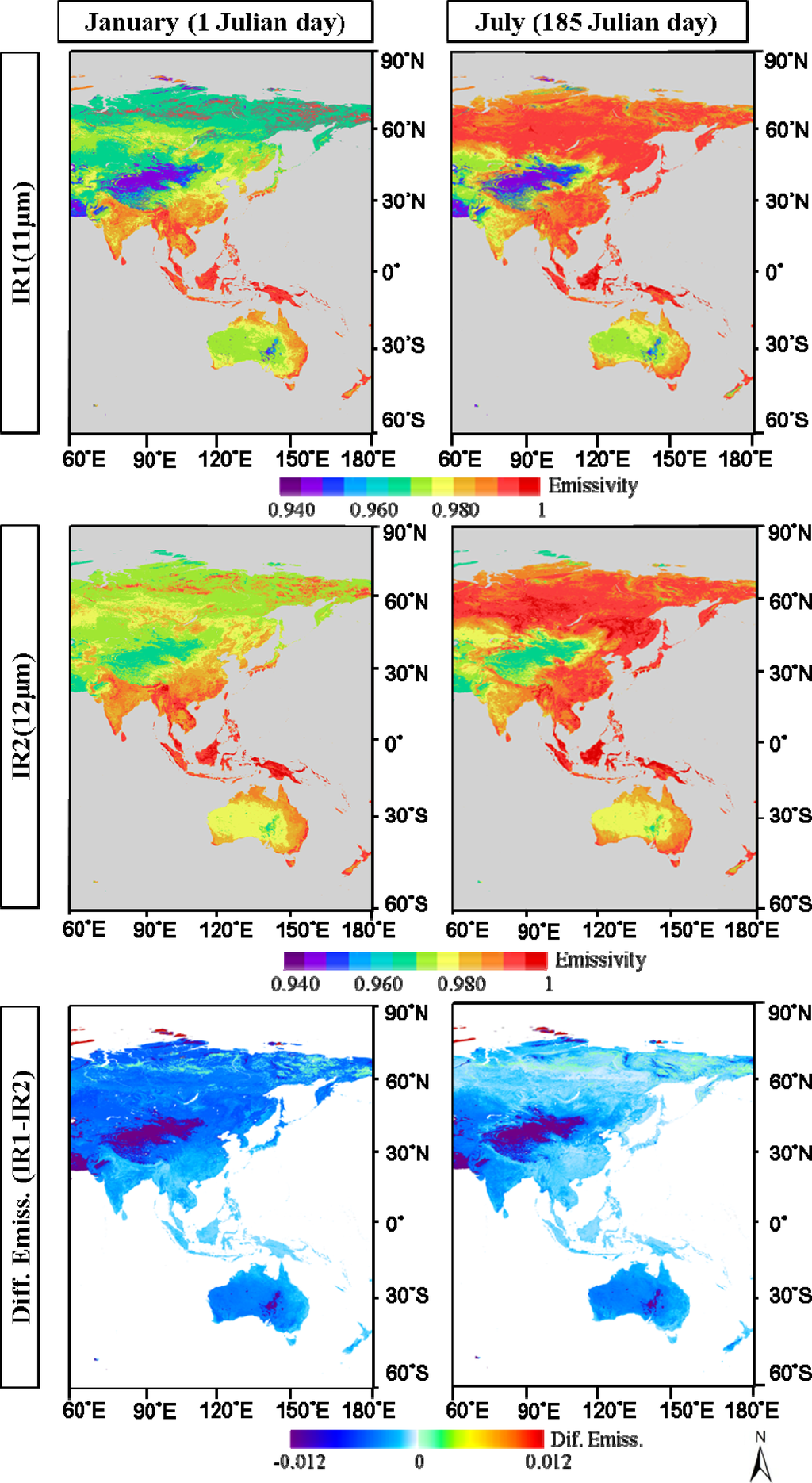
Figure 6.
Spatial distribution of surface emissivity and differences in surface emissivity for COMS IR1 and IR2 during the first half of January and July. Values were derived using the vegetation cover method (VCM).
4. Retrieval of LST Data and Evaluation of the Results
LST was only retrieved when the pixel was masked clear from COMS cloud mask data given by KMA’s National Meteorological Satellite Center. The preliminary quality of the COMS cloud masking algorithm was given by Choi et al. [51]. Additionally, some improvements were applied to the cloud mask algorithm in recent years after operational retrieval from COMS data [52].
As ground observations of LST were very limited, the collocated MODIS LST data were used to estimate the precision of the LST retrieved from COMS data as in Frey et al. [53]. Frey et al. [53] also cross-compared the four-year LST from AVHRR and MODIS for the pixels stuck to certain homogeneity criteria. They found that differences between two LST showed both a diurnal and an annual pattern, with some irregular patterns. Furthermore, mean annual absolute differences were relatively low: only 2.2 K for the daytime and 1.4 K for the night-time scenes, with a 0.99 coefficient of determination (R2). The quality of MODIS LST data is well documented in the literature [16,27–29]. The bias and RMSE of MODIS LST Version 5 are 1 K and less than 0.7 K when the LST range from −10 °C to 58 °C and atmospheric column water vapor ranges from 0.4 to 3.5 cm [16]. However, it was reported that the accuracy of LST was degraded in the case of heavy aerosol loadings and in the barren region in summer months [48].
Because temporal variation of LST can be substantial, especially during the daytime under dry conditions, only comparable MODIS LST data with time differences less than ±5 min were used in this study (MOD11_L2, MYD11_L2; Version5). Although ±5 min is not a short time-frame to use in LST comparisons, particularly during the daytime, we used this threshold for data inclusion to allow for the acquisition of an adequate number of evaluation samples. Furthermore, evaluation was only applied to MODIS LST data, where all the 25 (5 × 5) MODIS pixels were clear, based on the MODIS quality flag (mandatory-QA-flag is “00” or “01” and data-quality-flag is “00”) given at the each pixel, because spatial resolutions for COMS IR1 and IR2 data were 4 km at the corresponding nadir points. Although Deneke and Roebeling [54] and Bechtel et al. [8] showed that the evaluation could be improved if the point spread function was considered instead of just averaging the pixels, we simply averaged the 25 pixels of MODIS LST data.
Figures 7 and 9 show the spatial distribution of COMS LST and MODIS LST data and their differences for a few selected days during each season (three days and three nights). The images were constructed by compositing the collocated LST data for the selected days, because the observational area of MODIS changes according to its orbital path. The white color indicates pixels that were covered by clouds based on the flag data. The COMS-derived LST data showed a very similar spatial distribution to the LST data derived by MODIS, irrespective of what month or time of day the data were collected. As a result, differences between the two LST datasets were generally <5 K, irrespective of the geographic location and time except for the case of southern China. Although there were no obvious systematic patterns in the LST data differences, a closer analysis showed that negative differences were more prevalent during the nighttime than daytime. The latitudinal gradient for LST was weak or reversed during the daytime of the summer season, unlike in other seasons. This may have been caused by different thermal capacities of the soil surface, whereby there were more rapid and larger responses of LST in dry or sparsely vegetated regions than in wet or vegetated regions for similar insolation levels. Furthermore, the surface emissivity is impacted by the level of soil moisture [5,19].
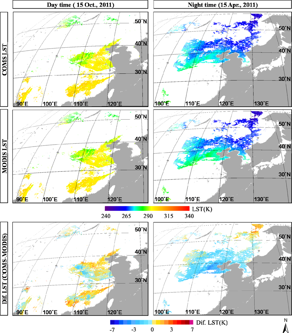
Figure 7.
Spatial distribution of COMS LST and Moderate Resolution Imaging Spectroradiometer (MODIS) LST data and their differences for two select days during autumn and spring (15 October 2011 and 15 April 2011).
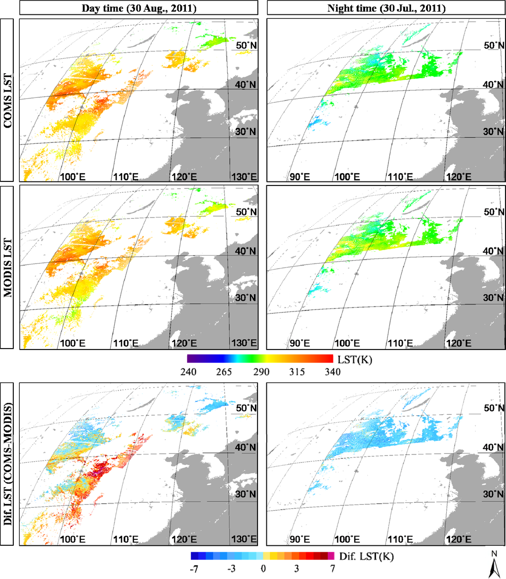
Figure 8.
Spatial distribution of COMS LST and MODIS LST data and their differences for two select days during summer (30 August 2011 and 30 July 2011).
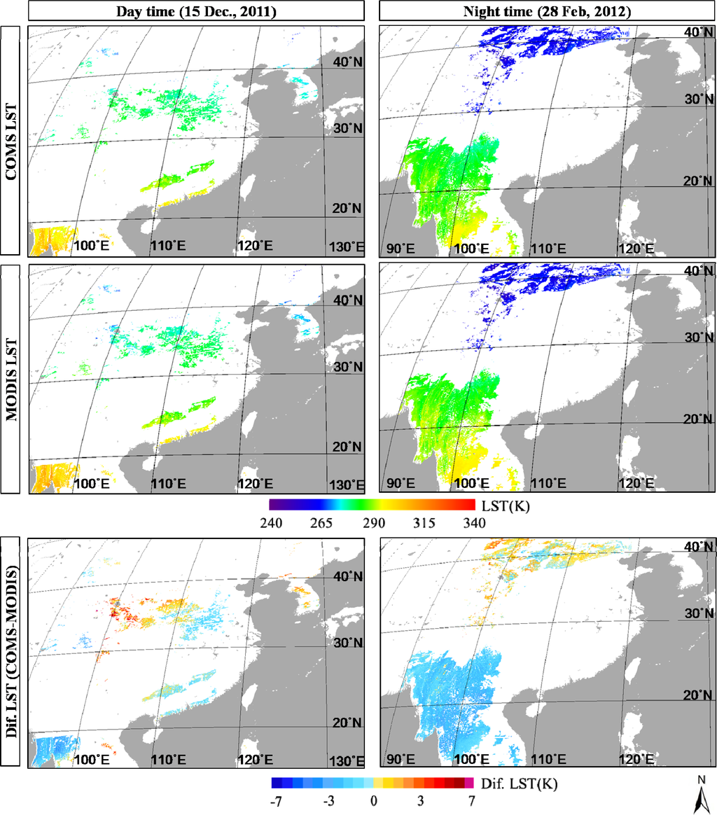
Figure 9.
Spatial distribution of COMS LST and MODIS LST data and their differences for two select days during winter (15 December 2011 and 28 February 2012).
The CSW algorithm overestimated the LST by more than +5 K when compared to MODIS LSTs for southwest China. When we consider that the time difference between the two satellite observations was short (less than ±5 min), the large spatial and temporal variations observed for LST differences might have been caused by differences in the viewing geometry of the two satellites, COMS and Terra/MODIS. Furthermore, navigation errors of the satellites and differences in surface emissivities may have contributed to the large LST differences. In the future, it would be valuable to conduct more research to establish what leads to the large LST differences, particularly during the daytime hours of the summer months.
Figure 10 shows a scatter plot of MODIS LST and COMS LST data for selected months. In general, the COMS LST data agreed well with the MODIS LST data without regard to the LST values ranging from 250 K to 330 K, and we observed no obvious systematic patterns in the LST data differences. However, a number of pixels showed a large discrepancy between the two LST datasets, which may have been caused by the differences in the SZA of two satellites, cloud masking or navigation accuracy issues.
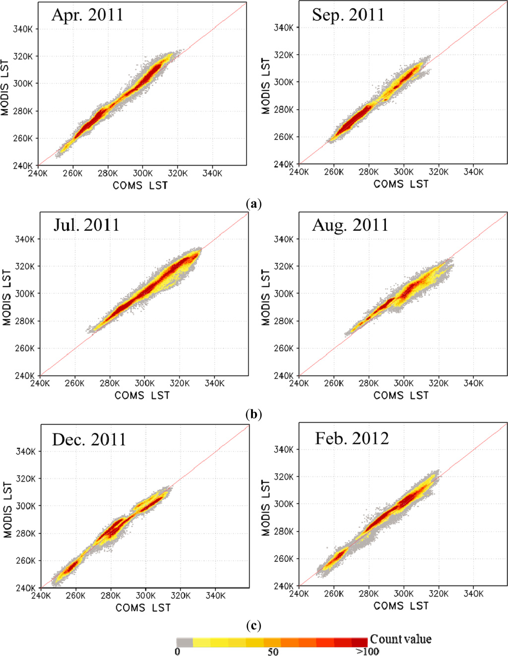
Figure 10.
Scatter plot of COMS LST vs. MODIS LST for the selected months: (a) April and September 2011; (b) July and August 2011; (c) December 2011 and February 2012.
A summary of the evaluation results obtained from comparing the COMS LST data to the MODIS LST data is presented in Table 3. Although the estimation capabilities of the CSW algorithm clearly depended on what month and time of day the data were collected, the monthly mean correlation between COMS LST and MODIS LST data was very high (average value of 0.988) and stable (the correlation coefficient ranged from 0.920 to 0.996). In general, the monthly mean biases were less than ±2.4 km except for the daytime of July. Additionally, the monthly mean RMSEs were less than ±3.5 km except for the months of May (daytime) and January (nighttime) irrespective of months and time. In general, the correlation coefficient and RMSE for nighttime data were systematically better than data collected during the daytime. However, the CSW algorithm systematically underestimated the nighttime LST values as compared to those taken during the daytime. These evaluation results show that the CSW algorithm can retrieve accurate LST data that would be appropriate for use in various applications irrespective of what months the data are collected in. However, attempts should be made to minimize the dependency of the estimation capabilities on the time of day that the data are collected to ensure the consistent retrieval of accurate LST data in the future.
Table 3.
Evaluation results comparing COMS LST data to MODIS LST data during the day and night times. Corr. Coeff., correlation coefficient.
5. Summary
We developed an SW-type LST retrieval algorithm from the initial data collected by the Korean geostationary satellite, COMS. The algorithm, termed CSW, was developed through radiative transfer model simulations under various atmospheric profiles derived from TIGR data, SZAs, surface emissivity values and surface lapse rate conditions using MODTRAN4. The estimation capabilities of the CSW LST algorithm were evaluated for various impacting factors, and the retrieval accuracy of COMS LST data was evaluated with the collocated MODIS LST data. For evaluation, averaged 5 × 5 MODIS LST data with time differences of less than ±5 min were used. The surface emissivity values of the two SW channels were generated by a VCM that assumed pixels were composed of soil and vegetation.
In general, the CSW algorithm estimated the LST distribution relatively well (averaged bias = 0.00 K, RMSE = 1.41 K, correlation coefficient = 0.99) for the given atmospheric and surface conditions. However, the estimation capabilities of the CSW algorithm were clearly impacted by large BTDs and surface lapse rates, particularly during the early morning hours and at noon. The impacts of large BTDs and surface lapse rates were enhanced by SZA. However, the impacts of surface emissivity on two thermal channels were not systematic and easily discernible. The VCM method reproduced spatiotemporal variations of surface emissivity reasonably well. The emissivity of IR2 was slightly greater than that of IR1 over the whole study area, but this difference was especially pronounced over desert and sparsely vegetated regions.
The CSW algorithm was able to reasonably retrieve the spatially distributed LST data compared to MODIS LST data irrespective of what months or time of day the data were collected. The one-year evaluation results with the collocated MODIS LST data showed that the retrieval capabilities of the CSW algorithm are more or less promising (annul mean bias = −1.009 K, RMSE = 2.613 K, correlation coefficient = 0.988). However, there were some relatively large variations in the monthly mean bias and RMSE for a few different months and times of day. These results suggest that the retrieval capabilities of the CSW algorithm could benefit from further improvements prior to using the algorithm in various applications, including regeneration of coefficients based on the critical impacting factors and investigation of the co-linearity between MODIS and COMS LST products. Additionally, the collection of more in situ observations of LST for different land covers and weather conditions could greatly help to improve the future assessments of the quantitative accuracy of the COMS LST data, because the MODIS LST data is not ground truth data [16,28,40,55].
Acknowledgments
This research was supported by the Korean Meteorological Administration Research and Development Program under Grant CATER 2012-2067. The one-year COMS Level-1B data and MODIS LST data were provided by the National Meteorological Satellite Center, the Korean Meteorological Administration and the National Aeronautics and Space Administration, respectively.
Conflict of Interest
The authors declare no conflict of interest.
References and Notes
- Price, J.C. Land surface temperature measurements from the split-window channels of the NOAA 7 AVHRR. J. Geophys. Res 1984, 89, 7231–7237. [Google Scholar]
- Wan, Z.; Dozier, J. A generalized split-window algorithm for retrieving land-surface temperature measurement from space. IEEE Trans. Geosci. Remote Sens 1996, 34, 892–905. [Google Scholar]
- Prata, A.J.; Cechet, R.P. An assessment of the accuracy of land surface temperature determination from the GMS-5 VISSR. Remote Sens. Environ 1999, 67, 1–14. [Google Scholar]
- Bodas-Salcedo, A.; Ringer, M.; Jones, A. Evaluation of the surface radiation budget in the atmospheric component of the Hadley Centre Global Environmental Model (HadGEM1). J. Clim 2008, 17, 4723–4748. [Google Scholar]
- Becker, F.; Li, Z.-L. Surface temperature and emissivity at various scales: Definition, measurement and related problems. Remote Sens. Rev 1995, 12, 225–253. [Google Scholar]
- Peres, L.; DaCamara, C.C. Land surface temperature and emissivity estimation based on the two-temperature method: Sensitivity analysis using simulated MSG/SEVIRI data. Remote Sens. Environ 2004, 91, 377–389. [Google Scholar]
- Neteler, M. Estimating daily land surface temperature in mountainous environments by reconstructed MODIS LST data. Remote Sens 2010, 2, 333–351. [Google Scholar]
- Bechtel, B.; Zakšek, K.; Hoshyaripour, G. Downscaling land surface temperature in an Urban area: A case study for Hamburg, Germany. Remote Sens 2012, 4, 3184–3200. [Google Scholar]
- Soliman, A.; Duguay, C.; Saunders, W.; Hachem, S. Pan-arctic land surface temperature from MODIS and AATSR: Product development and intercomparison. Remote Sens 2012, 4, 3833–3856. [Google Scholar]
- Kerr, Y.H.; Lagouarde, J.P.; Imbernon, J. Accurate land surface temperature retrieval from AVHRR data with use of an improved split window. Remote Sens. Environ 1992, 41, 197–209. [Google Scholar]
- Han, K.S.; Viau, A.A.; Anctil, F. An analysis of GOES and NOAA derived land surface temperatures estimated over a boreal forest. Int. J. Remote Sens 2004, 25, 4761–4780. [Google Scholar]
- Suh, M.S.; Kim, S.H.; Kang, J.H. A comparative study of algorithms for estimating land surface temperature from MODIS data. Kor. J. Remote Sens 2008, 24, 65–78. [Google Scholar]
- Trigo, I.; Peres, L.; DaCamara, C.C.; Freitas, S. Thermal land surface emissivity retrieved from SEVIRI/Meteosat. IEEE Trans. Geosci. Remote Sens 2008, 46, 307–315. [Google Scholar]
- Valor, E.; Caselles, V. Mapping land surface emissivity from NDVI: Application to European, African, and South American areas. Remote Sens. Environ 1996, 57, 164–184. [Google Scholar]
- Seemann, S.W.; Borbas, E.E.; Knuteson, R.O.; Stephenson, R.; Huang, H.-L. Development of a global infrared land surface emissivity database for application to clear sky sounding retrievals from multispectral satellite radiance measurements. J. Appl. Meteorol. Climatol 2008, 47, 108–123. [Google Scholar]
- Wan, Z. New refinements and validation of the MODIS land-surface temperature/emissivity products. Remote Sens. Environ 2008, 112, 59–74. [Google Scholar]
- Hulley, G.C.; Hook, S.J.; Baldridge, A.M. Validation of the North American ASTER land surface emissivity database (NAALSED) version 2.0 using pseudo-invariant sand dune sites. Remote Sens. Envrion 2009, 113, 2224–2233. [Google Scholar]
- Inamdar, A.K.; French, A. Disaggregation of GOES land surface temperatures using surface emissivity. J. Geophys. Res 2009, 36, L02408. [Google Scholar] [CrossRef]
- Li, Z.; Li, J.; Jin, X.; Schmit, T.J.; Borbas, E.E.; Goldberg, M.D. An objective methodology for infrared land surface emissivity evaluation. J. Geophys. Res 2010, 115, D22308. [Google Scholar] [CrossRef]
- MODIS UCSB Emissivity Library. Available online: http://www.icess.ucsb.edu/modis/EMIS/html/em.html (accessed on 13 May 2013).
- Jet Propulsion Laboratory: ASTER Spectral Library. Available online: http://speclib.jpl.nasa.gov/ (accessed on 13 May 2013).
- Loveland, T.R.; Reed, B.C.; Brown, J.F.; Ohlen, D.O.; Zhu, Z.; Yang, L.; Merchant, J.W. Development of a global land cover characteristics data base and IGBP DISCover from 1 km AVHRR data. Int. J. Remote Sens 2000, 21, 1251–1277. [Google Scholar]
- Wang, K.C.; Liang, S.L. Evaluation of ASTER and MODIS land surface temperature and emissivity products using long-term surface longwave radiation observations at SURFRAD sites. Remote Sens. Environ 2009, 113, 1556–1565. [Google Scholar]
- Kang, J.H.; Suh, M.S.; Kwak, C.H. Land cover classification over East Asia using Recent MODIS NDVI data (2006–2008). Kor. J. Atmos. Sci 2010, 20, 415–426. [Google Scholar]
- Terra/MODIS. Available online: https://lpdaac.usgs.gov/products/modis_products_table (accessed on 13 May 2013).
- MSG/SEVIRI. Available online: http://www.eumetsat.int/Home/Main/DataProducts/Land/index.htm?l=en (accessed on 13 May 2013).
- Wan, Z.; Zhang, Y.; Zhang, Q.; Li, Z. Validation of the land-surface temperature products retrieved from Terra Moderate Resolution Imaging Spectroradiometer data. Remote Sens. Environ 2002, 83, 163–180. [Google Scholar]
- Wan, Z.; Zhang, Y.; Zhang, Q.; Li, Z.-L. Quality assessment and validation of the MODIS global land surface temperature. Int. J. Remote Sens 2004, 25, 59–74. [Google Scholar]
- Sohrabinia, M.; Rack, W.; Zawar-Reza, P. Analysis of MODIS LST compared with WRF Model and in situ Data over the Waimakariri River Basin, Canterbury, New Zealand. Remote Sens 2012, 4, 3501–3527. [Google Scholar]
- Pinker, R.T.; Sun, D.; Hung, M.-P.; Li, C.; Basara, J.B. Evaluation of satellite estimates of land surface temperature from GOES over the United States. J. Appl. Meteorol. Climatol 2009, 48, 167–180. [Google Scholar]
- Hong, K.O.; Suh, M.S.; Kang, J.H. Development of a land surface temperature-retrieval Algorithm from MTSAT–1R data. Asia Pac. J. Atmos. Sci 2009, 45, 411–422. [Google Scholar]
- Tang, B.; Bi, Y.; Li, Z.L.; Xia, J. Generalized split-window algorithm for estimate of land surface temperature from Chinese geostationary FengYun meteorological satellite (FY–2C) data. Sensors 2008, 8, 933–951. [Google Scholar]
- Korea Meteorological Administration. Development of Meteorological Data Processing Systems of Communication, Ocean and Meteorological Satellite (V); KMA: Seoul, Korea, 2008. [Google Scholar]
- Hong, K.O.; Suh, M.S.; Kang, J.H. Improvement of COMS land surface temperature retrieval algorithm. Korean J. Remote Sens 2009, 25, 507–515. [Google Scholar]
- Korea Meteorological Administration. Retrieval of Land Surface Information from Satellite Data and Their Application; KMA: Seoul, Korea, 2012. [Google Scholar]
- Berk, A.; Anderson, G.P.; Acharya, P.K.; Chetwynd, J.H.; Bernstein, L.S.; Shettle, E.P.; Matthew, M.W.; Adler-Golden, S.M. MODTRAN4 Users’s Mannual; Air Force Research Laboratory: Hanscom AFB, MA, USA, 1999. [Google Scholar]
- Verhoef, W.; Bach, H. Simulation of hyperspectral and directional radiance images using biophysical and atmospheric radiative transfer models. Remote Sens. Environ 2003, 87, 23–41. [Google Scholar]
- Guanter, L.; Richter, R.; Kaufmann, H. On the application of the MODTRAN4 atmospheric radiative transfer code to optical remote sensing. Int. J. Remote Sens 2009, 30, 1407–1424. [Google Scholar]
- Jiménez-Muñoz, J.C.; Sobrino, J.A.; Mattar, C.; Franch, B. Atmospheric correction of optical imagery from MODIS and Reanalysis atmospheric products. Remote Sens. Environ 2010, 114, 2195–2210. [Google Scholar]
- Sobrino, J.A.; Romaguera, M. Land surface temperature retrieval from MSG1–SEVIRI data. Remote Sens. Environ 2004, 92, 247–254. [Google Scholar]
- Laboratoire de Météorologie Dynamique. Available online: http://ara.lmd.polytechnique.fr/htdocs-public/products/TIGR/TIGR.html (accessed on 13 May 2013).
- Coll, C.; Caselles, V. A split-window algorithm for land surface temperature from advanced very high resolution radiometer data: Validation and algorithm comparison. J. Geophys. Res 1997, 102, 16697–16713. [Google Scholar]
- Sobrino, J.A.; Raissouni, N. Toward remote sensing methods for land cover dynamic monitoring: Application to Morocco. Int. J. Remote Sens 2000, 21, 21353–21366. [Google Scholar]
- Sun, D.; Pinker, R.T. Retrieval of surface temperature from the MSG-SEVIRI observations: Part I. Methodology. Int. J. Remote Sens 2007, 28, 5255–5272. [Google Scholar]
- Gu, Y.; Rose, W.I.; Bluth, G.J.S. Retrieval of mass and sizes of particles in sandstorms using two MODIS IR bands: A case study of April 7, 2001 sandstorm in China. Geophys. Res. Lett. 2003, 30. [Google Scholar] [CrossRef]
- Peres, L.F.; DaCamara, C.C. Emissivity maps to retrieve land-surface temperature from MSG/SEVIRI. IEEE Trans. Geosci. Remote 2005, 43, 1834–1844. [Google Scholar]
- Sobrino, J.A.; Jiménez-Muñoz, J.C.; Sòria, G.; Romaguera, M.; Guanter, L.; Moreno, J.; Plaza, A.; Martínez, P. Land surface emissivity retrieval from different VNIR and TIR sensors. IEEE Trans. Geosci. Remote 2008, 46, 316–327. [Google Scholar]
- Trigo, I.F.; Monteiro, I.T.; Olesen, F.; Kabsch, E. An assessment of remotely sensed land surface temperature. J. Geophys. Res 2008, 113, D17108. [Google Scholar] [CrossRef]
- Momeni, M.; Saradjian, M.R. Evaluating NDVI-based emissivities of MODIS bands 31 and 32 emissivities derived by Day/Night LST algorithm. Remote Sens. Environ 2007, 106, 190–198. [Google Scholar]
- Park, K.H.; Suh, M.S. Inter-comparison of three land surface emissivity data sets (MODIS, CIMSS, KNU) in the Asian-Oceanian regions. Kor. J. Remote Sens 2013, 29, 219–233. [Google Scholar]
- Choi, Y.-S.; Ho, C.-H.; Ahn, M.-H.; Kim, Y.-M. An exploratory study of cloud remote sensing capabilities of the Communication, Ocean and Meteorological Satellite (COMS) imagery. Int. J. Remote Sens 2007, 28, 4715–4732. [Google Scholar]
- Choi, Y.-S. Personal Communication. 27 November 2012.
- Frey, C.M.; Kuenzer, C.; Dech, S. Quantitative comparison of the operational NOAA AVHRR LST product of DLR and the MODIS LST product V005. Int. J. Remote Sens 2012, 33, 7165–7183. [Google Scholar]
- Deneke, H.M.; Roebeling, R.A. Downscaling of METEOSAT SEVIRI 0.6 and 0.8 μm channel radiances utilizing the highresolution visible channel. Atmos. Chem. Phys 2010, 10, 9761–9772. [Google Scholar]
- Wang, W.; Liang, S.; Meyers, T. Validating MODIS land surface temperature products using long-term nighttime ground measurements. Remote Sens. Environ 2008, 112, 623–635. [Google Scholar]
© 2013 by the authors; licensee MDPI, Basel, Switzerland This article is an open access article distributed under the terms and conditions of the Creative Commons Attribution license ( http://creativecommons.org/licenses/by/3.0/).