Ground-Based Hyperspectral Characterization of Alaska Tundra Vegetation along Environmental Gradients

Abstract

Remote sensing has become a valuable tool in monitoring arctic environments. The aim of this paper is ground-based hyperspectral characterization of Low Arctic Alaskan tundra communities along four environmental gradients (regional climate, soil pH, toposequence, and soil moisture) that all vary in ground cover, biomass, and dominating plant communities. Field spectroscopy in connection with vegetation analysis was carried out in summer 2012, along the North American Arctic Transect (NAAT). Spectral metrics were extracted, including the averaged reflectance and absorption-related metrics such as absorption depths and area of continuum removal. The spectral metrics were investigated with respect to “greenness”, biomass, vegetation height, and soil moisture regimes. The results show that the surface reflectances of all sites are similar in shape with a reduced near-infrared (NIR) reflectance that is specific for low-growing biomes. The main spectro-radiometric findings are: (i) Southern sites along the climate gradient have taller shrubs and greater overall vegetation biomass, which leads to higher reflectance in the NIR. (ii) Vegetation height and surface wetness are two antagonists that balance each other out with respect to the NIR reflectance along the toposequence and soil moisture gradients. (iii) Moist acidic tundra (MAT) sites have “greener” species, more leaf biomass, and green-colored moss species that lead to higher pigment absorption compared to moist non-acidic tundra (MNT) sites. (iv) MAT and MNT plant community separation via narrowband Normalized Difference Vegetation Index (NDVI) shows the potential of hyperspectral remote sensing applications in the tundra.

1. Introduction

Time series of satellite data from the Advanced Very High Resolution Radiometer (AVHRR) from 1982 to 2010 have shown an increase in the Normalized Difference Vegetation Index (NDVI), an index of vegetation biomass and greenness, of about 8% for the northern hemisphere tundra [1]. This greening trend is caused by increased tundra productivity, which is thought to be mainly a response to climate warming [2–5]. The Arctic is warming at nearly double the general planetary rate [6]. Extrapolation of the NDVI trend assigning biomass data from two Arctic transects indicates an average 19.8% increase in above-ground tundra biomass during the AVHRR NDVI record (1982–2010) [4]. This has major implications for tundra ecosystems, including changes in active layer depth, permafrost and thermokarst distribution, carbon cycling, hydrology, and wildlife [7].

Monitoring of Arctic landscapes is therefore important. Due to the remoteness and large area of the tundra biome, satellite and aerial remote sensing provide the best prospective tools for land-cover mapping and change detection [8–11]. However, the short vegetation growing period and therefore accelerated phenology, frequent cloud cover, high standing water and surface water coverage, and extreme illumination conditions (sun zenith angles in arctic latitudes always larger than 43°) challenges optical remote sensing of vegetation in the Arctic [10,12,13].

Several studies have shown the capability of multi-spectral satellite and aerial remote sensing data to extract biophysical plant parameters. The studies for the North American tundra biome mainly used broadband NDVI indices [4,10,12,14–19]. Horler et al. [20] noticed that broad-band based remote sensing may not be adequate to extract sharp reflectance changes in narrow spectral regions, such as the “red-edge”, between the red and near-infrared. The technical development in airborne and satellite imaging spectroscopy sensors like AVIRIS (Airborne Visible and Infrared Imaging Spectrometer) [21], CHRIS/Proba (Compact High Resolution Imaging Spectrometer/Project for On-Board Autonomy) [22], EO-1/Hyperion (Earth Observing 1/Hyperion instrument) [23], and the upcoming German EnMAP (Environmental Mapping and Analysis Program) satellite mission [24] opens the door for new methods that can use the entire spectral feature space of imaging spectroscopy [25,26].

Reflectance from vegetated surfaces is highly differentiated by wavelength. The visible (VIS) wavelengths (400–700 nm) are strongly influenced by the pigment absorption of the plants in different wavelength regions [27,28]. The main pigment groups are chlorophylls and carotenoids. The light absorption for photosynthesis is mainly done by chlorophylls, with absorption maxima in the blue and red wavelength regions. Carotenoids have their absorption maxima in the blue and green wavelength regions and the group of anthocyanins in the green wavelength region [28]. The reflectance in the near-infrared (NIR) wavelength region (700–1,400 nm) is mainly influenced by plant cell structure and vegetation biomass. Multiple scattering of radiation between air and cell wall in leaf tissue leads to high reflectance values in this region referred to as the NIR reflectance plateau [29]. This sharp reflectance contrast between VIS and NIR is commonly used in remote sensing for calculating vegetation indices using combinations of red and NIR wavelength regions [30–32].

The use of hyperspectral data can improve the prediction of biophysical variables [33,34], but there are limited imaging spectroscopy data of North American tundra landscapes available. This is a common shortcoming all over the Arctic [13]. Field spectroscopy is a valuable tool to gain ground-based hyperspectral data.

The objective of this paper is to characterize and distinguish Low Arctic Alaskan tundra vegetation communities along important environmental gradients via field spectroscopy. To provide an overview on the spectral characteristics assists the classification and analyses of tundra vegetation using satellite hyperspectral imagery. The North American Arctic Transect (NAAT) sites provide representative measurement grids covering gradients of zonal climate, soil moisture, and soil pH. The gradients along the Low-Arctic part of the NAAT show therefore changes in vegetation biomass, height of vegetation, leaf mass, and surface moisture. We investigated if spectral characteristics are linked to geoecological characteristics of the Low Arctic tundra vegetation and their change along the gradients.

2. Material & Methods

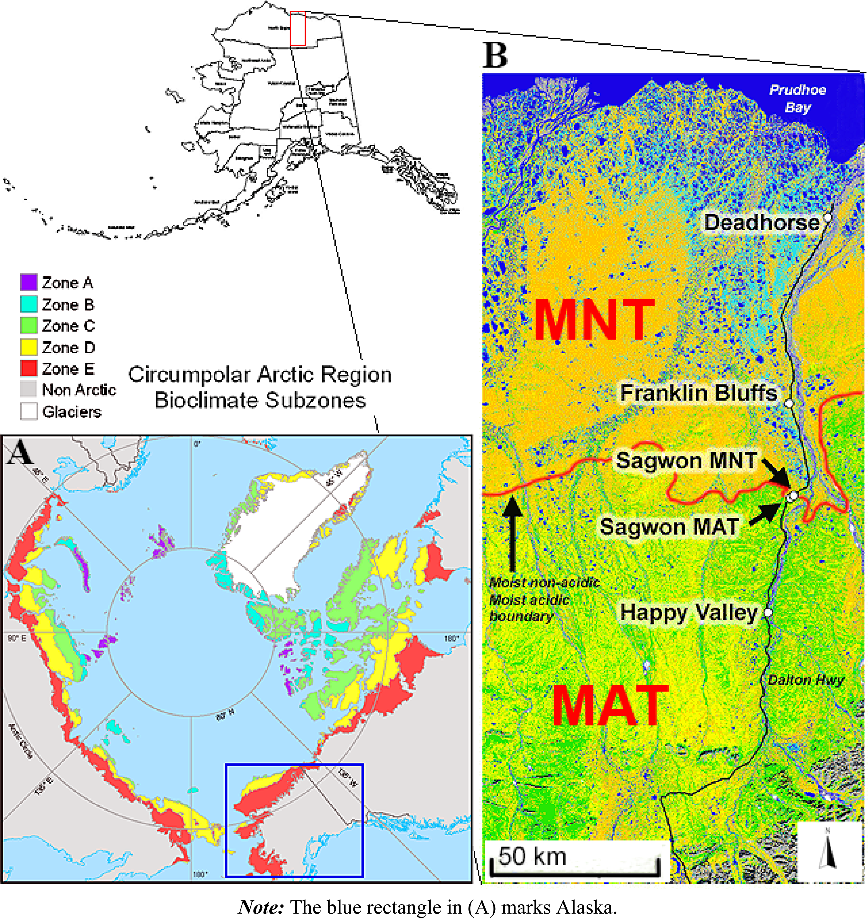
2.1. Study Area

The Circumpolar Arctic Vegetation Map (CAVM) divides the Arctic tundra into five bioclimate subzones (A–E) based on a combination of summer temperatures and vegetation [35] (Figure 1A). Subzones D and E compose the Low Arctic. The North American Arctic Transect (NAAT), established in 2002–2006, follows the Dalton Highway, crossing Alaska’s North Slope [36], and extends into the western Canadian High Arctic islands [37]. It includes study locations in all five bioclimate subzones. Along the 250 km Low Arctic part of this transect, four NAAT study locations were established—Deadhorse (transition subzone C/D), Franklin Bluffs (subzone D), Sagwon Hills (transition subzone D/E), and Happy Valley (subzone E) (Figure 1B). All study locations contain at least one 100 m² mapped grid with homogeneous vegetation, including a good representation of the zonal vegetation in subzones D and E and transition types. Nine study sites were investigated in summer 2012, during the EyeSight-NAAT-ALASKA expedition [38]. We carried out field spectroscopy measurements in addition to updating the vegetation descriptions and soil moisture measurements at each site.

A detailed description of plant communities and geology of the Low Arctic portion of the NAAT can be found in Kade et al. [39], and Vonlanthen et al. [40] provide this analysis for the High Arctic part of the NAAT. A synthesis of NAAT publications is in Walker et al. [41,42], and considerable other information is available in on-line data reports [43].

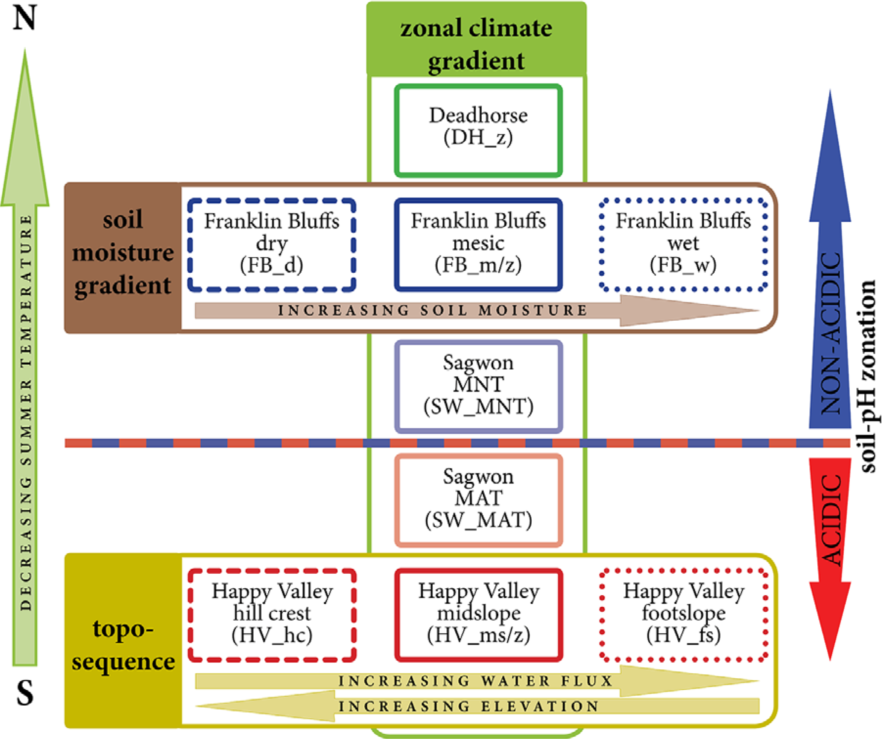
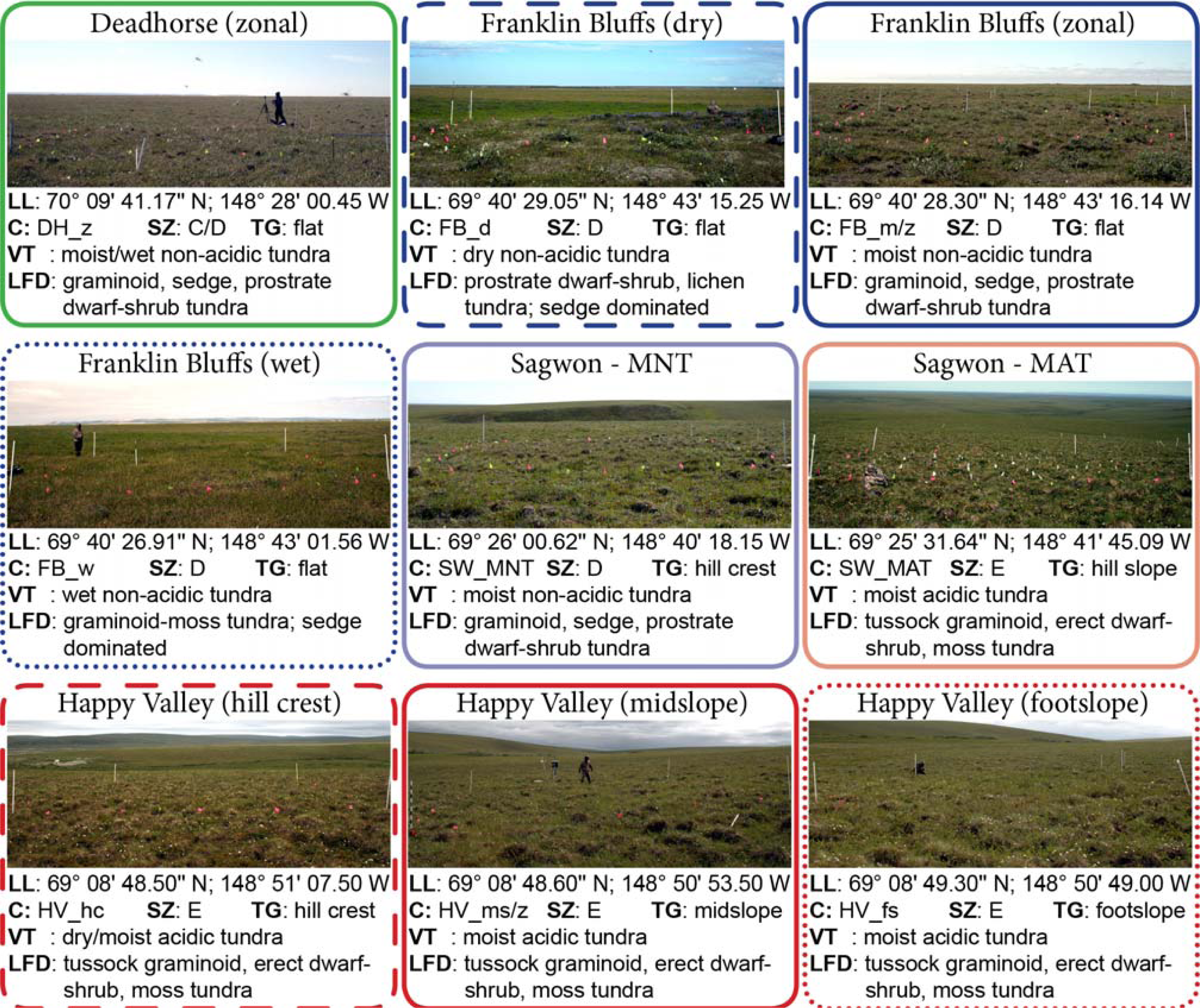
2.2. Environmental Gradients/Zones and Vegetation Description

The nine study sites represent arctic tundra vegetation communities along four arctic environmental gradients and zones: summer temperature, soil pH, soil moisture, and topography. The latitudinal climate gradient (bioclimate subzones) influences vegetation along the whole Low Arctic transect, the soil pH zoning reflects a substrate division between acidic and non-acidic soils (Figure 1B). The toposequence (hillslope) gradient is most relevant at landscape scales influencing lateral water fluxes, and the soil moisture gradient is influential at the site scale as well as being apparent at all scales [44]. These gradients are, however, not orthogonal. There is the general temperature gradient and pH zonation from north to south with further variations related to moisture and topography. In order to assign a study site to a conceptual gradient, the main influencing factor was used. Figure 2 shows the nine study sites in relationship to the four conceptual environmental gradients and zones. Figure 3 outlines the main geoecological characteristics of the nine test sites.

The regional climate gradient with differences in the summer warmth index (SWI) is well represented by the five zonal sites of this study (Deadhorse, Franklin Bluffs-mesic, Sagwon-MNT, Sagwon-MAT, and Happy Valley-midslope) (Figures 2 and 3). The SWI is the sum of mean monthly temperatures greater than 0 °C [19]. The term “zonal” refers to vegetation under the influence of the regional climate, without the influences of extremes of snow, soil properties, moisture, or disturbances [45]. Walker et al. [35] describe the zonal vegetation in bioclimate subzones D and E for the circumpolar Arctic in detail. The main influence of the regional climate is the increase in phytomass towards the south.

An important soil pH boundary occurs at Sagwon [46]. Two test sites (Sagwon-MNT and Sagwon-MAT) were established at the Sagwon Hills study location to capture this variation in the patterning between Subzones D and E (Figures 2 and 3). This boundary separates the predominantly moist acidic tundra (MAT) south of the boundary from the predominantly moist non-acidic tundra (MNT) to the north. The boundary is close to but not coincident with a physiographic boundary separating the Arctic Foothills to the south from the Arctic Coastal Plain to the north [47]. The MAT plant community is Sphagno-Eriophoretum vaginati [48] (also called “acidic tussock tundra” or “tussock-sedge, dwarf-shrub, moss tundra” [35]) and corresponds to the zonal plant community of bioclimate subzone E in northern Alaska. It occurs widely across the foothills of northern Alaska on old upland surfaces not glaciated during the Last Glacial Maximum. The vegetation is composed of a mixture of tussock sedges, deciduous dwarf shrubs, evergreen dwarf shrubs, a few forbs, mosses, and lichens. The MNT plant community is Dryado integrifoliae-Caricetum bigelowii [35] (also called “nontussock sedge, dwarf-shrub, moss tundra” [35]) and corresponds to the zonal plant community of bioclimate subzone D in northern Alaska. It occurs on circumneutral to basic soils in association with silty loess that is blown from the major rivers in the eastern part of the Arctic Coastal Plain. The dominant plants in MNT are sedges, prostrate and hemi-prostrate evergreen dwarf shrubs, prostrate dwarf deciduous shrubs, scattered erect dwarf deciduous shrubs, several forbs, mosses, and lichens. An important component of the MNT is the abundant nonsorted circles (frost boils), which are small patterned ground features caused by soil frost heave and covering large parts of most MNT surfaces [37,49].

In order to analyze the vegetation changes along a toposequence, the zonal test site in Happy Valley (Happy Valley-midslope) was extended by two additional sites in this study area (Happy Valley-hill crest and Happy Valley-footslope) (Figures 2 and 3). Analysis of variation along short hillslope gradients is a primary tool for describing how water movement downslope over long periods of time affects soil development and ecological properties [50,51]. Such “toposequences” are part of the underlying conceptual framework for describing Arctic vegetation at the landscape scale for the circumpolar Arctic [35]. The vegetation, soils, patterned ground features and biomass of the small east-facing hill slope were previously characterized and mapped during several studies at this location [39,52–55]. The grids are positioned on the hill crest, at 325 m, the midslope, at 310 m (representing also the zonal Happy Valley site), and the footslope, at 300 m. The main difference between the hillcrest and the zonal midslope community is that the hill crest is somewhat drier with more nonsorted circles that have the plant community Cladino-Vaccinietum vitis-idaeae [39], which has similar species composition to Sphagno-Eriophoretum vaginati, but with no Sphagnum and higher cover of grass, nontussock sedges, prostrate evergreen dwarf shrubs, the moss Racomitrium lanuginosum, and lichens. The footslope has a greater abundance of (and taller) erect dwarf shrubs.

The fourth environmental gradient is the change in soil moisture and was investigated at the Franklin Bluffs study area (Figures 2 and 3). This area in the northern part of the Alaska portion of the NAAT transect is on the central Arctic Coastal Plain, a land of thaw-lakes, ice-wedge polygons, and braided river systems. Micro-topographic variations of a few centimeters to a few meters control the vegetation patterns associated with patterned-ground features, thaw lake margins and ancient river terraces. The three Franklin Bluffs study sites can be characterized as wet, mesic (zonal), and dry. They were used in previous studies to characterize the vegetation, soils, and patterned ground associated with differences in soil moisture [39,54,55]. The wet site is on an old floodplain of the Sagavanirktok River that is situated about 1 m below a small river terrace. It has a marshy Scorpidium scorpioides-Carex aquatilis plant community [39] with large, more-or-less barren nonsorted circles. The dominant plants of the wet site are sedges, a few forbs including horsetails, and mosses, and considerable cover of water during most summers. The mesic site is composed of a mix of the zonal Dryado integrifoliae-Caricetum bigelowii community [39] and a frost-boil subassociation, Junco biglumis-Dryadetum integrifoliae pedicularetosum [39], which is drier with more bare soil, lichens and forbs. The dry site is on better-drained soils near the edge of the terrace, where the main plant community is dominated by prostrate dwarf shrubs, cushion, and mat forbs, and a large component of bare soils and lichens.

2.3. Data Acquisition and Pre-Processing

Field data were collected at all nine study sites from 23 June to 22 July 2012 [38]. Since we revisited already existing, marked, and well described plots with a size of 10 × 10 m, the sampling design for the vegetation and surface properties update was predetermined [54]. We estimated the percentage cover of the individual dominant plant species and grouped the species into height strata in order to calculate mean percentage cover of the strata. We used the scalar cover estimates of the Braun-Blanquet approach used in the original description [56]. The vertical structure was analyzed by measuring the average height of the strata. The vegetation at all sites can be divided into three strata: the photosynthetic part of the moss layer (L1) with a height up to 2 cm; the mainly vascular herbaceous plant and dwarf shrub layer (L2) with a height up to 15 to 30 cm; and the top layer (L3) composed of taller shrubs with up to 50 cm height. We needed to define a new type of cover measurement for the three vegetation strata (L1, L2, and L3) that simulates the percentage cover of what the nadir-measuring field spectrometer would “see”. This simulated percentage nadir-cover is calculated from the true areal cover by leaving the full percentage cover of the highest plant canopy layer (L3) which is the first layer that a nadir-viewing sensor measures. Then, we estimated the percentage cover of the second highest plant canopy layer (L2). Finally, subtracting the top two strata (L3, L2) from the overall percentage cover of vegetated (non-lichen) leaves the remaining percentage nadir-cover for the lowest vegetation layer (L1). This conversion does not change the percentage cover contributions of L2 and L3 as measured in the field. However, the moss layer (L1) has a much lower percentage nadir-cover value than the common 90 to 100% true cover, but represents the contribution of this layer that is measured by field spectroscopy. For pixel-related remote sensing applications, the fractional vegetation cover (FVC) summing up to 100% is the useful parameter for many environmental and climate-related applications. In order to describe the vegetation color, we used Munsell Plant Tissue Color Charts. The Munsell color notation system ranks colors based on three color dimensions: hue, value (lightness), and chroma (purity) [57]. The average soil moisture content was calculated from 30 randomly distributed point measurements throughout the grid using a TDR (Time Domain Reflectrometry) soil moisture meter (Campbell) with a 15 cm rod length.

For the field spectroscopy each 100 m² study grid was divided into quadrats of 1 × 1 m. The averaged reflectance of all quadrats represents the spectral reflectance at the scale of the whole grid at the 10 × 10 m scale. For the surface radiometric measurements two GER1500 portable field spectroradiometers (Spectra Vista Corporation, Poughkeepsie, NY, USA) were used. The GER1500 measures radiance across the wavelength range of 350–1,050 nm, with sampling intervals of 1.5 nm (calibrated in May 2011) and a radiance accuracy of 1.2 × 10⁻¹ W·cm⁻²·nm⁻¹·sr⁻¹ [58]. In order to increase the signal-to-noise ratio, 32 individual measurements were averaged per one target scan. To minimize variations in the target reflectance due to sun zenith angle changes, all measurements at one study location have been performed under the same sun zenith angle (Happy Valley = 47°, Sagwon = 48°, Franklin Bluffs = 47°, Deadhorse = 49°) and during clear-sky conditions. To ensure that all measurements are comparable, the sun zenith angle change between the four study locations was 2°. All measurements were taken between 29 June and 11 July 2012, ensuring that the vegetation at all sites was in the same phenological state near peak growing season [10].

A Spectralon^® white panel (Labsphere, Inc., North Sutton, NH, USA) was used for white reference normalization using the recommendation of Milton [59]. Target reflectance measurements were taken by measuring the radiance of the target and the white reference panel within a short timespan (less than 10 min under clear-sky conditions). To reduce the short-term temporal changes in irradiation (sky- and atmospheric effects) we developed a cos-conical dual-beam approach, where two GER-1500 spectroradiometers simultaneously measured the radiance of the target and the sky irradiance. One spectrometer with a cosine diffusor foreoptic mounted at a height of 1.80 m was placed near the site pointing vertically upwards to measure the downwelling total sky irradiance. Care was taken to ensure that the sensor was not masked or shadowed. The second spectrometer was used to measure the target radiance. This spectrometer used a 4° field of view (FOV) foreoptic at a distance of 1.40 m to the middle of each 1 × 1 m quadrat, resulting in a measurement area with approximately 10 cm diameter. To operate two spectrometers in a dual-beam modus requires careful intercalibration of the instruments [59,60]. Instead of using the recorded irradiance directly, we used the irradiance spectra with the aim to interpolate the radiance measurement of the reference panel to the time of the target measurement. It is assumed that changes in the irradiance over the time period affect the radiance measurements of the reference panel to a similar degree [61]. This approach has already been used by various groups, but mostly with a sunphotometer with limited spectral bands for irradiance recording [61,62].

2.4. Data Analysis

The reflectance spectra of the field spectroscopy were stored in a database. One averaged reflectance spectrum with standard deviations was calculated for each site using the footprint measurements of the one hundred quadrats. The results for the nine tundra study sites are nine averaged reflectances (n = 9) representing the sites at a 10 × 10 m scale. We used the following analysis techniques to extract spectral metrics from the average reflectance spectra for comparison between the study sites: (i) we calculated the averaged reflectance values for two broad wavelength bands, VIS band (400–700 nm) and NIR band (700–1,050 nm), in order to compare the variations along the environmental gradients. (ii) we analyzed the NIR plateau with the maximum reflectance at 750 nm and 1,020 nm as well as the difference between the two (delta). For the analysis of the VIS part of the reflectance spectra we used (iii) the “relative absorption depth” approach [63] in the blue and red wavelength regions and (iv) the continuum removal normalization technique [64] using a common baseline for the blue and red wavelength absorption regions in order to compare the differences in pigment absorption. The continuum removal technique was developed for geological applications, but can also be used for estimating biochemical concentrations [65,66] or vegetation differentiation [67]. A detailed description of this technique can be found in Kokaly and Clark [65]. From the continuum removed spectra we calculated the maximum band depth and the area of the absorption feature in the blue (400–550 nm) and red (550–750 nm) wavelength regions. All calculated spectral features of the averaged reflectance spectra were then investigated in comparison to the biophysical vegetation parameters. The vegetation parameters are average vegetation height, average top height, overall above-ground biomass, and Munsell color. The term “average top height” is the average height of the top layer in the canopy, which is mostly formed by shrubs. We investigated if the hue and value codes of the Munsell color information of a plant community are linked to its dominant color [68].

Another method to link biophysical vegetation parameters to the reflectance spectra is the usage of vegetation indices (VI). Vegetation indices can be conceptually simple but effective (e.g., band ratios) or complex, using methods such as support vector machines [69], which incorporate more data from the spectral feature space. Most of the VIs for the analysis of structural vegetation properties have been developed for broadband sensor systems but have hyperspectral equivalents [32]. Hyperspectral vegetation indices (HVIs) use narrowband features, which can only be captured by hyperspectral instruments [32]. Research by Thenkabail et al. [34,70] has shown that, due to data redundancy in the hyperspectral signal, a small number of specific hyperspectral narrowbands (HNBs) have enough information to determine structural vegetation characteristics. Therefore, hyperspectral two-band vegetation indices (HTBVI) based on normalized difference between the bands are used as a data-mining tool in this study.

In preparation for the EnMAP hyperspectral space mission we resampled the field spectroscopy data to EnMAP sensor bands using the spectral response curves of the sensor. In order to assess all possible EnMAP band combinations, we calculated the HTBVI according to Equation (1) [31,34,71]

$${\mathit{HTBVI}}_{i,j}=\frac{(R_{{\mathit{band}}_j}-R_{{\mathit{band}}_i})}{(R_{{\mathit{band}}_j}+R_{{\mathit{band}}_i})}$$

(1)

where R is the reflectance of the EnMAP bands, and correlated the HTBVI values with biomass. This approach is already well known and used by various research groups [31,71,72]. We used the tool SpInMine (Spectral Index Data Mining Tool) [73], which is implemented in the EnMAP-Box software [74]. Biomass (kg/100 m²) for all nine study sites was obtained from Raynolds et al. [54].

The results of the 4,560 unique HTBVIs from the 96 EnMAP bands (424–1,074 nm) are shown in Figure 4. Hotspots of correlation between the HTBVIs and biomass are located with one band in the VIS region and one band in the NIR region. Band combinations with one band in the blue region and one band in the green to red region also show high correlations. Due to the small sample size of n = 9, the optimal HNBs cannot be further constrained. Additionally, other methods to reduce the data redundancy, such as partial least squares (PLS) or principal component analysis (PCA), are not possible with such a small sample size.

Therefore, we decided to try an alternative approach. One of the most robust and commonly used VI is the NIR and red wavelength based NDVI, which is also a normalized difference index [31,32,75,76] and is calculated according to Equation (2).

$$\mathit{NDVI}=\frac{({\text{R}}_{\text{NiR}}-{\text{R}}_{\text{red}})}{({\text{R}}_{\text{NiR}}+{\text{R}}_{\text{red}})}$$

(2)

The NDVI based on broadband wavelengths bands has successfully been used in numerous studies along the NAAT in order to show vegetation changes and as a surrogate for various biophysical properties of vegetation, such as biomass, leaf-area index (LAI), and intercepted photosynthetically active radiation (IPAR) [4,12,17,19,77]. To be comparable to the studies, which used mostly broadband NDVI based on AVHRR, we resampled the field spectroscopy data to AVHRR sensor bands using the response curves of the sensor (

Table 1. Center wavelengths and band width of the broadband and narrowband Normalized Difference Vegetation Index (NDVIs) used in this study, based on the spectral response curves of the Advanced Very High Resolution Radiometer (AVHRR) and Environmental Mapping and Analysis Program (EnMAP) sensors.

NDVI	Sensor	Sensor Band	Center Wavelength (nm)	Band Width (nm)
NDVIAVHRR (broadband)	AVHRR/3	red: band 1	630	100
		NIR: band 2	865	275
NDVI47_59 (narrowband)	EnMAP	red: band 47	672	6.5
		NIR: band 59	756	6.5
NDVI47_73 (narrowband)	EnMAP	red: band 47	672	6.5
		NIR: band 73	864	8
NDVI47_101 (narrowband)	EnMAP	red: band 47	672	6.5
		NIR: band 101	1,018	11

). Then we compared this broadband NDVI with three narrowband NDVIs compiled from simulated EnMAP data (Table 1). To analyze the performance of the HVIs, we linked the NDVI values to the above-ground biomass via regression analysis. In addition, the probability distributions of the broadband and narrowband NDVIs for each site were investigated in order to assess differences between MAT and MNT. The HNBs in the red and NIR wavelength regions for the three narrowband NDVIs have been chosen by assessment of the spectral metrics, based on research in optimal HNBs for vegetation analysis by Thenkabail et al. [34,70]. Where the central wavelength of the EnMAP red band (EnMAP band 47, center wavelength 672 nm) shows the maximum chlorophyll absorption, the NIR HNBs use the EnMAP NIR bands of the beginning of the NIR reflectance plateau (EnMAP band 59, center wavelength 756 nm), the central NIR reflectance plateau (EnMAP band 71, center wavelength 864 nm) and the maximum NIR reflectance (EnMAP band 101, center wavelength 1,020 nm). EnMAP band 59 at the beginning of the NIR reflectance plateau may be specifically sensitive to vegetation structure. The center wavelength of EnMAP band 71 equals the center wavelength of the AVHRR NIR band (865 nm). EnMAP band 101 is around the maximal NIR reflectance at the second NIR reflectance peak that is located behind the first NIR reflectance peak around 900 to 920 nm [78] and the water absorption band.

3. Results

The results were compiled following the environmental gradients concept (Figure 2). Figure 5 displays the averaged reflectance spectra of each site showing the general spectral characteristics of Alaskan Low Arctic tundra communities along the NAAT (

Table 2. Geoecological characteristics of the ninestudy sites. All parameters were collected during the EyeSight-NAAT-Alaska expedition 2012, except the values for SWI, soil pH and biomass, which were obtained from Raynolds et al. [54].

	Site Code	SWI (°C)	Soil Parameters		Vegetation Parameters			Munsell Color Information+				Detailed Vegetation Parameters (Nadir Cover)
			pH-Value	Moisture (Vol %)	Average Height (cm)*	Average Top Height (cm)Δ	Biomass (kg/100 m2)	Overall	L1	L2	L3	Soil Crust (%)□	L1 Cover (%)	L1 Height (cm)	L1 Description	L2 Cover (%)	L2 Height (cm)	L2 Description	L3 Cover (%)	L3 Height (cm)	L3 Description
Regional climate	DH_z	17.3	7.9	70	23	25	33.17	10Y (5/4)	5Y (6/8)	5GY (5/4)		10	20	<2	Moss	70	2–30	sedge & shrub	0	–	–
	FB_m/z	24.2	8.0	48	15	35	43.40	2.5GY (6/4)	5Y (6/8)	5GY (6/4)	5GY (5/6)	5	8	<2	Moss	82	2–15	sedge & shrub	5	15–40	shrub
	SW_MNT	26.5	7.7	39	8	45	56.30	7.5Y (7/8)	5Y (8/10)	5GY (6/6)	5GY (5/6)	3	64	<2	Moss	30	2–15	sedge & shrub	3	15–50	shrub
	SW_MAT	26.5	5.4	35	12	30	75.10	2.5GY (7/8)	2.5GY (8/10)	5GY (5/6)	5GY (5/4)	2	57	<2	Moss	40	2–25	tussock & shrub	1	25–35	shrub
	HV_ms/z	29.5	5.1	38	14	45	72.08	2.5GY (6/6)	2.5GY (8/10)	5GY (5/4)	5GY (5/4)	4	43	<2	Moss	48	2–20	tussock & shrub	5	20–50	shrub
Soil-pH (Sagwon)	SW_MNT	26.5	7.7	39	8	45	56.30	7.5Y (7/8)	5Y (8/10)	5GY (6/6)	5GY (5/6)	3	64	<2	Moss	30	2–15	sedge & shrub	3	15–50	shrub
	SW_MAT	26.5	5.4	35	12	30	75.10	2.5GY (7/8)	2.5GY (8/10)	5GY (5/6)	5GY (5/4)	2	57	<2	Moss	40	2–25	tussock & shrub	1	25–35	shrub
Topo-sequence	HV_hc	29.5	5.1	27	12	40	73.54	2.5GY (6/8)	2.5GY (8/10)	5GY (5/6)	5GY (5/6)	10	43	<2	Moss	45	2–20	tussock & shrub	2	20–45	shrub
	HV_ms/z	29.5	5.1	38	14	45	72.08	2.5GY (6/6)	2.5GY (8/10)	5GY (5/4)	5GY (5/4)	4	43	<2	Moss	48	2–20	tussock & shrub	5	20–50	shrub
	HV_fs	29.5	5.1	45	25	55	73.44	5GY (6/6)	2.5GY (8/10)	5GY (6/4)	5GY (5/4)	2	28	<2	Moss	50	2–25	tussock & shrub	20	25–60	shrub
Soil-moisture	FB_d	24.2	8.1	36	14	30	48.96	2.5GY (5/6)	5Y (6/8)	5GY (5/4)	5GY (5/6)	10	30	<2	Moss	40	2–15	sedge & shrub	20	15–35	shrub
	FB_m/z	24.2	8.0	48	15	35	43.40	2.5GY (6/4)	5Y (6/8)	5GY (6/4)	5GY (5/6)	5	8	<2	Moss	82	2–15	sedge & shrub	5	15–40	shrub
	FB_w	24.2	7.8	74	30	35	40.39	2.5GY (6/4)	5Y (6/8)	5GY (6/4)		10	10	<2	Moss	80	2–40	sedge & shrub	0	–	–

Note: The percentage cover of the vegetation height strata (L1, L2, and L3) are calculated as nadir-cover. Therefore, for example, the percentage cover of L1 does not equal the true coverage of the moss layer.

^*of the whole test site;

^Δmostly shrubs which form the top layer in the canopy;

⁺derived from Munsell Plant Tissue Color Charts;

^□areas which are vegetated by lichen (no barren soil)—in close relation to the appearance or remnants of nonsorted circles.

). The metrics of the spectral data analysis are shown in

Table 3. Metrics of the spectral data analysis.

		Average R (Broad Bands)		Max. R in NIR*			Relative Absorption Depth		Continuum Removed				NDVI's with SE
	Site Code	VIS (%) (400–700)	NIR (%) (700–1,050)	750 (%)	1,020 (%)	Delta R (1,020-750)	400–550 (blue)	550–750 (red)	Area 400–550	Area 550–750	Max. Blue Band Depth	Max. Red Band Depth	Broad NDVIAVHRR	Narrow 1 NDVI47_59	Narrow 2 NDVI47_73	Narrow 3 NDVI47_101
Regional climate	DH_z	5.9	21.4	17.8	25.2	7.4	0.40	0.68	8.7	48.4	0.11	0.43	0.48 (±0.01)	0.39 (±0.01)	0.48 (±0.01)	0.53 (±0.01)
	FB_m/z	5.8	24.6	21.3	28.9	7.6	0.41	0.98	11.9	64.5	0.15	0.55	0.55 (±0.01)	0.49 (±0.02)	0.56 (±0.01)	0.60 (±0.01)
	SW_MNT	5.6	24.4	20.2	28.9	8.7	0.44	0.92	14.2	58.3	0.17	0.52	0.55 (±0.01)	0.48 (±0.01)	0.56 (±0.01)	0.61 (±0.01)
	SW_MAT	5.1	24.4	21.7	27.5	5.8	0.53	1.17	17.6	68.9	0.21	0.60	0.59 (±0.01)	0.55 (±0.01)	0.61 (±0.01)	0.64 (±0.01)
	HV_ms/z	4.7	25.8	22.8	29.5	6.7	0.58	1.43	23.0	77.5	0.27	0.66	0.64 (±0.01)	0.60 (±0.01)	0.66 (±0.01)	0.68 (±0.01)
Soil-pH (all)	non acidic	5.8	23.2	19.8	27.1	7.3	0.41	0.86	10.8	57.8	0.14	0.50	0.53 (±0.01)	0.46 (±0.01)	0.53 (±0.01)	0.58 (±0.01)
	acidic	4.6	25.0	22.2	28.5	6.3	0.56	1.34	20.6	74.2	0.24	0.64	0.62 (±0.01)	0.59 (±0.01)	0.65 (±0.01)	0.67 (±0.01)
Soil-pH (Sagwon)	SW_MNT	5.6	24.4	20.2	28.9	8.7	0.44	0.92	14.2	58.3	0.17	0.52	0.55 (±0.01)	0.48 (±0.01)	0.56 (±0.01)	0.61 (±0.01)
	SW_MAT	5.1	24.4	21.7	27.5	5.8	0.53	1.17	17.6	68.9	0.21	0.60	0.59 (±0.01)	0.55 (±0.01)	0.61 (±0.01)	0.64 (±0.01)
Topo-sequence	HV_hc	4.7	23.0	20.1	26.4	6.3	0.52	1.21	19.1	68.7	0.22	0.61	0.60 (±0.01)	0.57 (±0.01)	0.63 (±0.01)	0.66 (±0.01)
	HV_ms/z	4.7	25.8	22.8	29.5	6.7	0.58	1.43	23.0	77.5	0.27	0.66	0.64 (±0.01)	0.60 (±0.01)	0.66 (±0.01)	0.68 (±0.01)
	HV_fs	4.5	26.9	24.0	30.5	6.5	0.62	1.60	22.5	81.8	0.27	0.69	0.67 (±0.01)	0.64 (±0.01)	0.69 (±0.01)	0.71 (±0.01)
Soil-moisture	FB_d	5.7	23.7	21.3	26.9	5.6	0.37	1.07	9.9	68.2	0.14	0.59	0.56 (±0.02)	0.52 (±0.02)	0.58 (±0.02)	0.61 (±0.02)
	FB_m/z	5.8	24.6	21.3	28.9	7.6	0.41	0.98	11.9	64.5	0.15	0.55	0.55 (±0.01)	0.49 (±0.02)	0.56 (±0.01)	0.60 (±0.01)
	FB_w	5.8	21.9	18.4	25.7	7.3	0.44	0.72	9.2	49.4	0.12	0.43	0.49 (±0.01)	0.40 (±0.01)	0.49 (±0.01)	0.53 (±0.01)

Note: R = reflectance; VIS = visible wavelength range; NIR = near-infrared wavelength range; VI = vegetation indices; SE = standard error;

^*of the average reflectance graph; numbers in table header are wavelengths in nm.

. Figure 6 displays the range of reflectance spectra of each site.

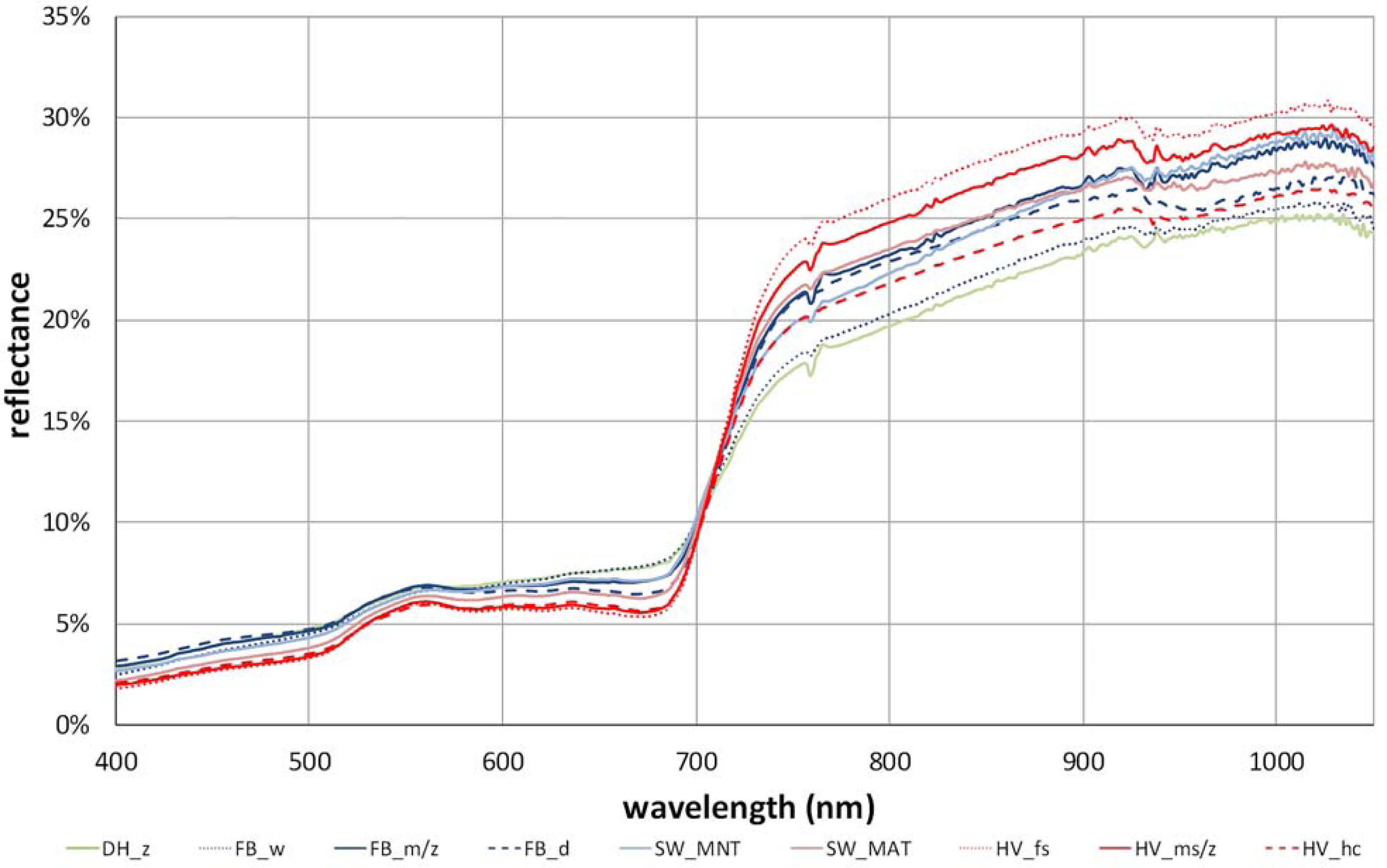
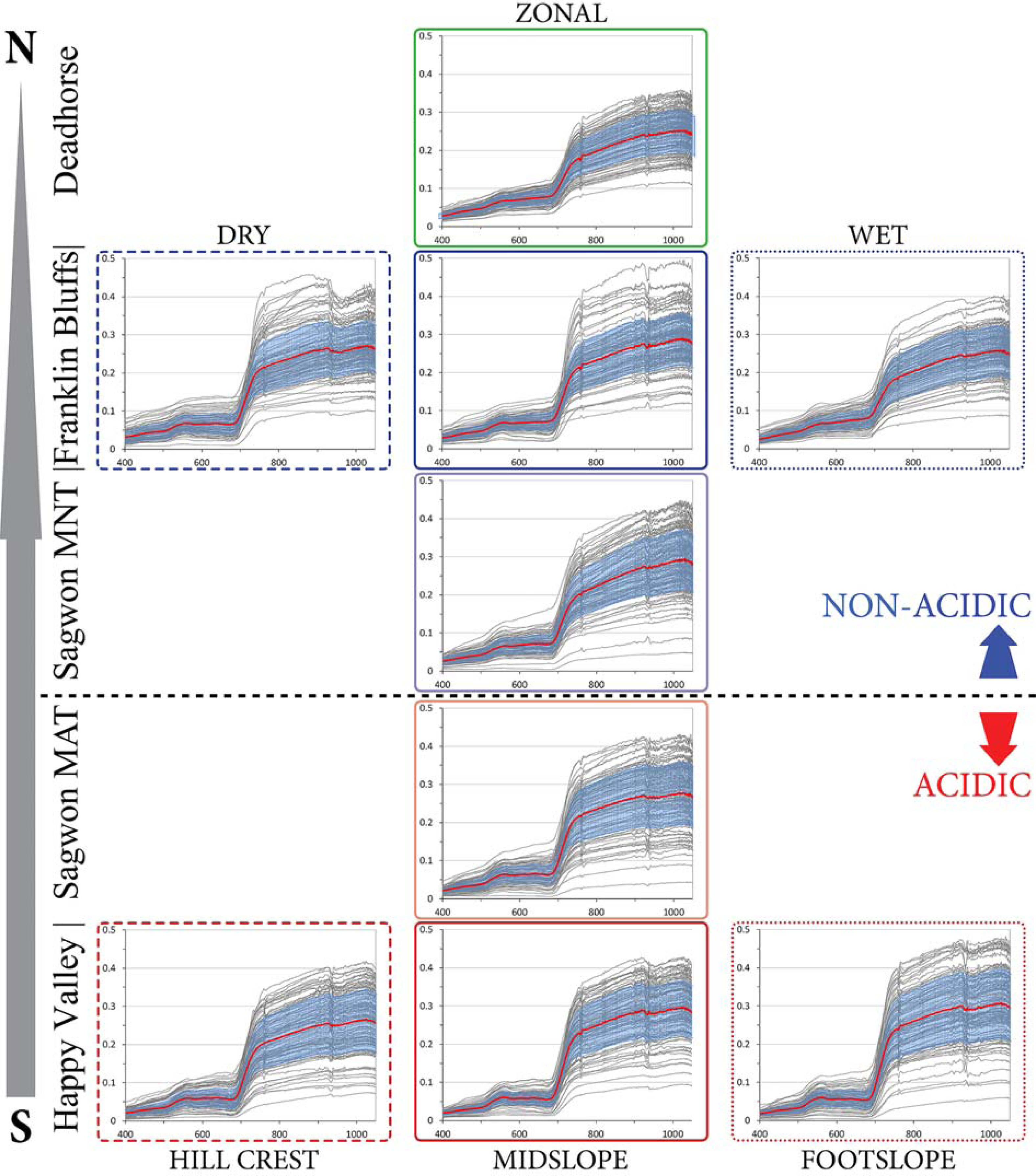
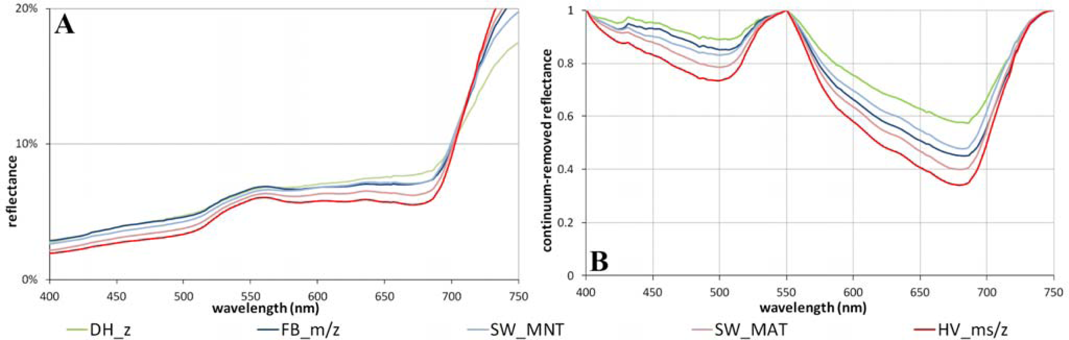
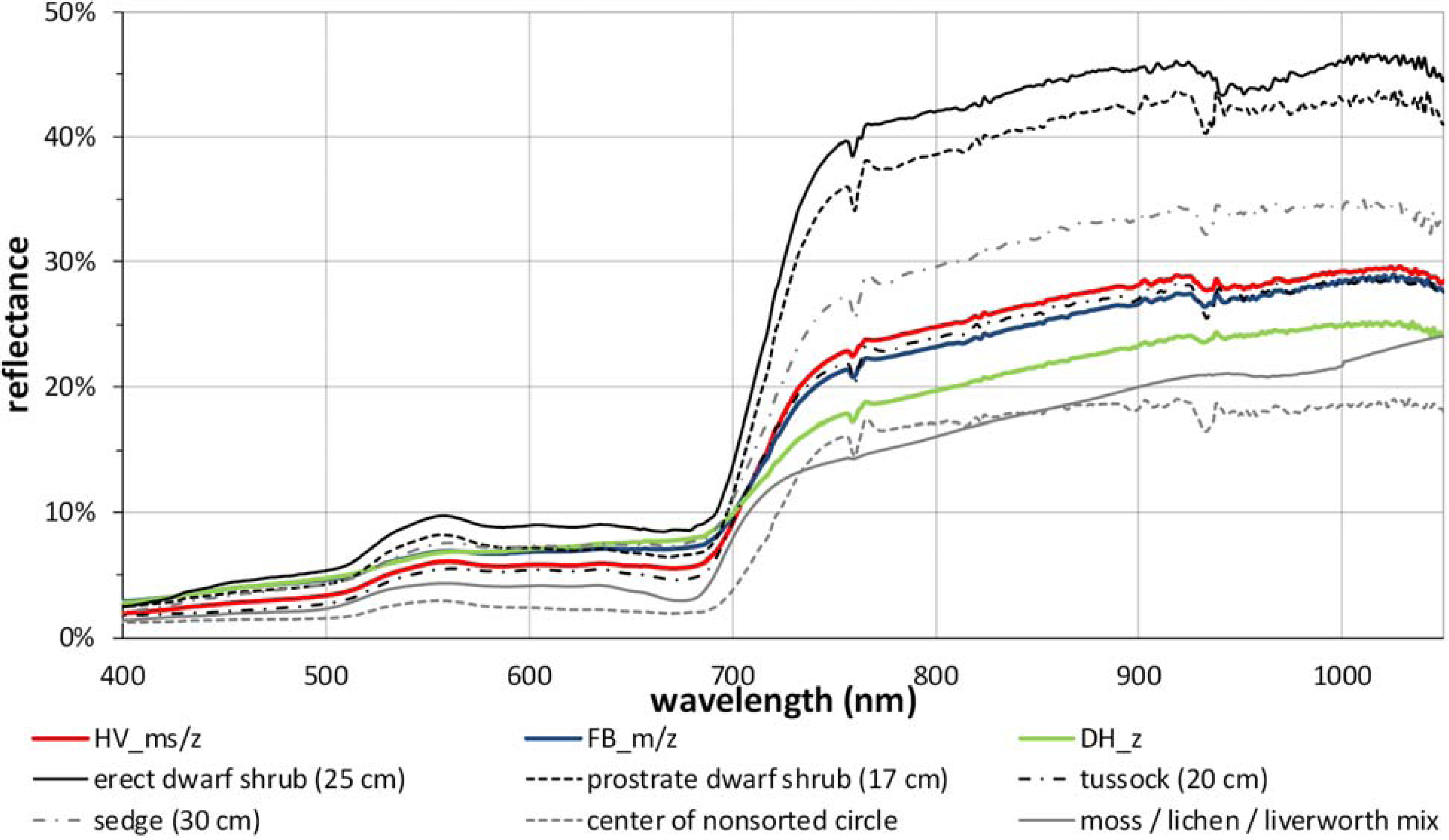
3.1. The Zonal Climate Gradient

The zonal climate gradient is defined by the SWI, which decreases from 29.5 °C at Happy Valley, 26.5 °C at Sagwon, 24.2 °C at Franklin Bluffs to 17.3 °C at Deadhorse (Table 2). This temperature (climate) gradient follows the latitude of the study locations from south to north. The mean vegetation heights range from 14 cm at Happy Valley (HV_ms/z), 8 to 12 cm at Sagwon (SW_MNT, SW_MAT), 15 cm at Franklin Bluffs (FB_m/z), and 23 cm at Deadhorse (DH_z). The average top height follows a different height trend, the heights increase towards the south. The top height at HV_ms/z, Sagwon (both sites) and FB_m/z are composed of shrubs, whereas the top height at DH_z is composed by fast-growing sedges. This also explains the higher mean value for vegetation height for DH_z, the most northern site, compared to the southern sites. However, the biomass including the moss layer considerably decreases towards the north, from 75.10 to 33.17 kg/(100 m²) (Table 2). The overall vegetation coverage (non-lichen) decreases from 98% in the south to 90% in the north. The non-vegetated areas in all test sites are never barren soil but are covered by soil crusts (lichen and bryophytes), which generally appear in the center of nonsorted circles.

The reflectance spectra of all five zonal sites are, in general, similar in shape but with an offset of up to one percentage point in the VIS. The offset in the VIS in reflectance increases towards the north. Therefore, the sites clearly differ by their VIS spectra. Both subzone E sites have the green reflectance peak as the local reflectance maxima, whereas the more northern sites have the reflectance maxima in the red wavelength region and a hardly noticeable green reflectance peak (Figure 7A).

The reflectance values of the 300 nm wide VIS band (Table 3) increase from 4.7% at HV_ms/z, 5.1% at SW_MAT, 5.6% at SW_MNT, 5.8% at FB_m/z to 5.9% at DH_z. The relative absorption depths of the zonal site inversely follow this latitudinal trend. The further south the site, the greater the absorption depth of the blue (400–550 nm) and red (550–750 nm) absorption features. The blue relative absorption depth increases from 0.40 at DH_z to 0.58 at HV_ms/z, and the absorption depth of the red feature increases from 0.68 at DH_z to 1.43 at HV_ms/z.

The spectral metrics derived from the continuum removal analysis also exhibit the same trend of increasing absorption in the blue and red wavelength regions along the climate gradient towards the south (Figure 7B). The area of the blue absorption feature increases from 8.7 at DH_z to 23.0 at HV_ms/z, and the maximum band depth at around 500 nm increases from 0.11 at DH_z to 0.27 at HV_ms/z. For the red absorption feature the area increases from 48.4 at DH_z to 77.5 at HV_ms/z, and the maximum band depth at around 680 nm increases from 0.43 at DH_z to 0.66 at HV_ms/z.

Each reflectance spectrum along the temperature gradient shows a similar shape with a steady NIR increase, and the further south the geographic location of the site, the higher is the NIR reflectance (Figure 5). None of the reflectance spectra has a well-developed NIR reflectance plateau. This trend is also noticeable in the 350 nm wide NIR band reflectance and the maximum reflectance at 750 nm and 1,020 nm (Table 3). The reflectance of the 350 nm wide NIR band increase from 21.4% at DH_z to 25.8% at HV_ms/z, and the maximum reflectance at 1,020 nm increases from 25.2% at DH_z to 29.5% at HV_ms/z.

Broadband narrowband NDVI values also show the latitudinal trend (Table 3). The broadband NDVI_AVHRR values increase from 0.48 at DH_z in the north to 0.64 at HV_ms/z in the south. Likewise, the three narrowband NDVI values increase from north to south, but with different intervals between the minima at DH_z and the maxima at HV_ms/z. The best separation of the sites occurs with NDVI_{47_101}, which uses the narrowband at 1,018 nm in the NIR (the NIR maximum) (Table 3). NDVI_{47_59}, using the narrowband at 756 nm in the NIR, shows the largest span between minimum and maximum (0.39 at DH_z and 0.60 at HV_ms/z). NDVI_{47_73} captures the separation between the sites similarly to the broadband NDVI.

The regression analyses of the spectral metrics as well as NDVI values and biomass show strong correlations with high coefficients of determination (R²) in all cases (Figure 8). The correlation of the relative absorption depths in the blue and red wavelength regions with biomass (Figure 8A,B) illustrates the good separation of the five zonal sites in the blue (R² = 0.80) and red (R² = 0.74) reflectances according to their geographical location. These high R² values occur also in the regression analyses of the continuum removed maximum band depths with biomass (Figure 8C,D). The comparison of broadband and narrowband NDVIs (Figure 8E–H) indicates that the narrowband NDVIs have similar to slightly higher correlations with biomass (NDVI_{47_59} = 0.81; NDVI_{47_73} = 0.83; NDVI_{47_101} = 0.80) compared to the broadband NDVI_AVHRR (R² = 0.80).

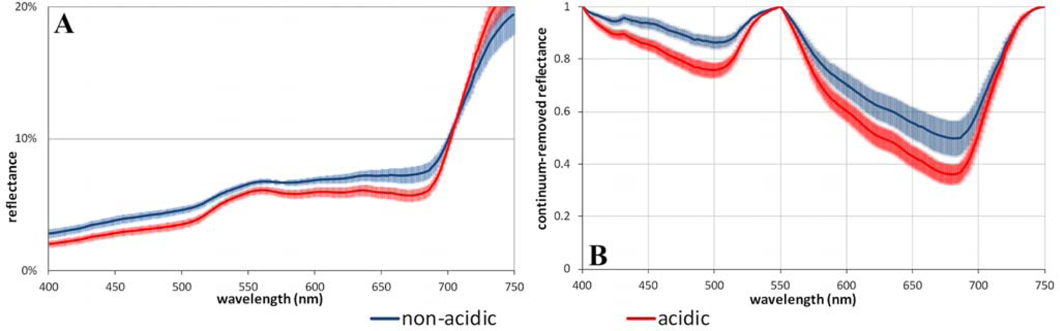
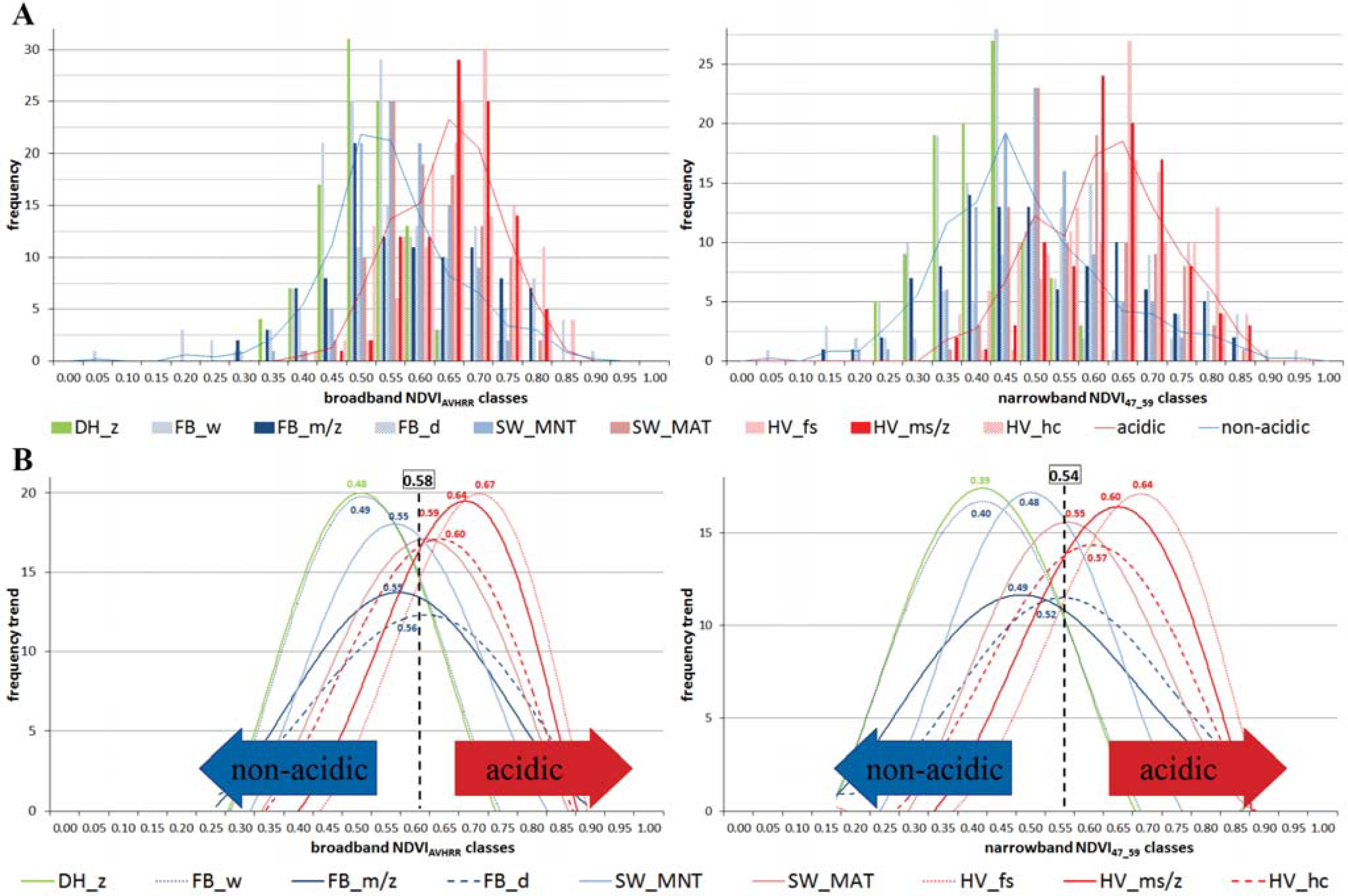
3.2. Acidic vs. Non-Acidic Tundra (Soil pH Zones)

Whereas all four acidic sites have soil pH values between 5.1 and 5.4, the five non-acidic sites have soil pH values between 7.7 and 8.1 (Table 2). The vegetation composition is mainly MAT at the acidic sites and MNT at the non-acidic sites. All non-acidic sites have overall vegetation coverage from 90% to 97%, whereas the range at the acidic sites is 90% to 98%.

All sites with acidic tundra (three sites at Happy Valley and Sagwon-MAT) have the green reflectance peak at 550 nm as the local reflectance maximum and a distinctive chlorophyll absorption dip at 680 nm in the VIS wavelength region. In contrast, the non-acidic sites (Sagwon-MNT, all sites at Franklin Bluffs, and Deadhorse) have the local reflectance maximum in the red wavelength region and have a hardly notable green reflectance peak (Figure 9A).

In the VIS wavelength range, the reflectance spectra of the non-acidic sites are clearly distinguishable from the acidic sites. This differentiation can also be seen directly at the soil pH boundary at Sagwon. The average reflectance value of the 300 nm wide VIS band of all acidic sites is 4.8% and of all non-acidic sites 5.8%. Directly at the soil pH boundary, the acidic Sagwon-MAT (SW_MAT) site has a reflectance of 5.1% vs. 5.6% at the non-acidic Sagwon-MNT (SW_MNT) site. Acidic tundra has an average relative absorption depth in the blue wavelength region of 0.56 (0.53 at SW_MAT), and non-acidic tundra has a depth of 0.41 (0.44 at SW_MNT). This difference increases for the relative absorption depth of the red wavelength region. On average the acidic sites have a relative absorption depth of 1.34 (1.17 at SW_MAT), and the non-acidic sites have depths of 0.86 (0.92 at SW_MNT). The continuum removal analysis also shows a clear separation of the study sites on acidic and non-acidic soils within the chlorophyll absorption maximum around 680 nm and chlorophyll/carotenoid absorption at 500 nm (Figure 9B). In both absorption features the acidic sites have deeper absorption than the non-acidic sites (Table 3). The area of the blue absorption feature of the acidic tundra is 20.6 (17.6 at SW_MAT) and of the non-acidic 10.8 (14.2 at SW_MNT), and the maximum band depth at around 500 nm of the acidic sites is 0.24 (0.21 at SW_MAT) and 0.14 (0.17 at SW_MNT) for the non-acidic sites. Additionally, the areas of the continuum removed red absorption features decrease from 74.2 for acidic tundra (68.9 for SW_MAT) to 57.8 for non-acidic (58.3 for SW_MNT). The maximum band depth in the continuum removal is 0.64 for acidic sites (0.60 for SW_MAT) and 0.50 for non-acidic (0.52 for SW_MNT).

Such a clear separation does not occur in the NIR reflectance. Here the reflectance spectra of the acidic and non-acidic sites show some overlap (Figure 5), especially of the sites close to the soil pH boundary at Sagwon. The reflectance values of the 350 nm wide NIR band are on average 25.0% for acidic soil sites (24.4% at SW_MAT) and 23.2% for non-acidic (24.4% at SW_MNT).

The results of the broadband and narrowband NDVI analysis (Table 3) show a clear separation of acidic and non-acidic tundra. Where acidic tundra has an average broadband NDVI_AVHRR of 0.62, non-acidic tundra has an average of 0.53. This partition is also detectable right at the soil pH boundary at Sagwon. The acidic SW_MAT site has a broadband NDVI_AVHRR of 0.59 and the non-acidic SW_MNT site a broadband NDVI_AVHRR of 0.55. All three narrowband NDVIs also show this separation between acidic and non-acidic tundra (Table 3). A broadband and narrowband NDVI histogram analysis indicates in all cases that the distributions of acidic and non-acidic sites are distinct, with acidic sites strongly skewed to the higher NDVI values (Figure 10A). In a direct comparison, NDVI_{47_59} shows the clearest separation between MAT and MNT in the probability distribution relative to the broadband NDVI_AVHRR. The average broadband NDVI_AVHRR of the acidic sites ranges from 0.59 to 0.67, whereas the broadband NDVI_AVHRR of the non-acidic sites ranges from 0.48 to 0.56 (Figure 10B). The separation value between acidic and non-acidic tundra in the broadband NDVI_AVHRR is 0.58. The narrowband NDVI_{47_59} has a separation value of 0.54, where the average NDVI_{47_59} values of MAT range from 0.55 to 0.64 and of MNT from 0.40 to 0.52.

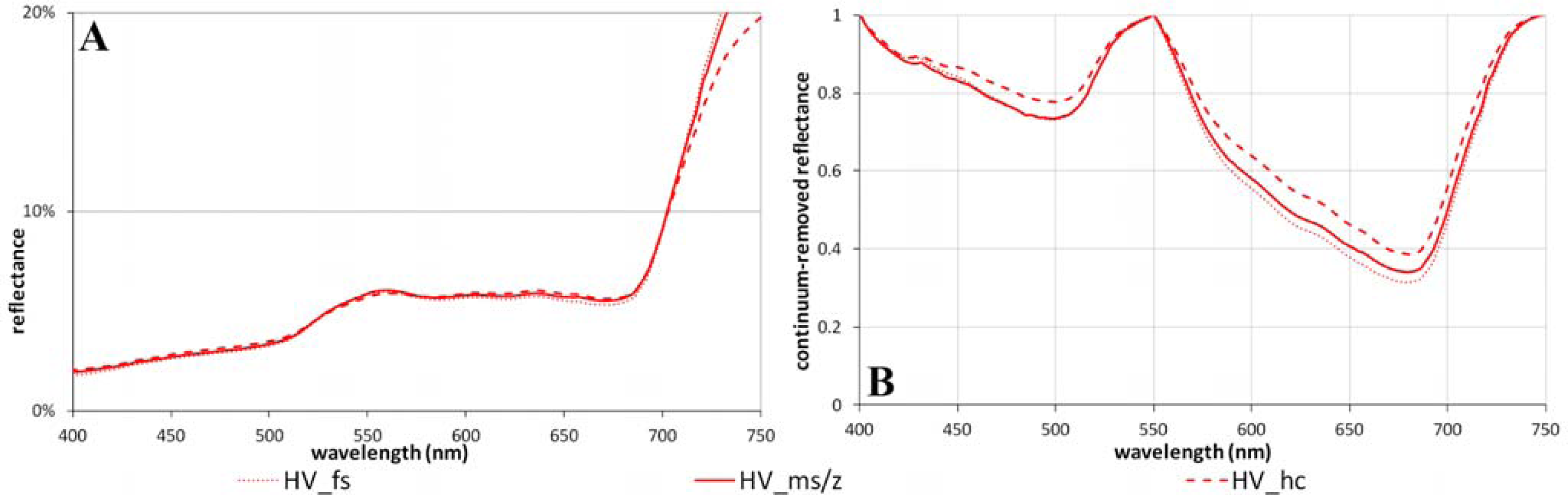
3.3. The Toposequence at Happy Valley (Subzone E)

At the Happy Valley study location all three sites forming the toposequence have an identical soil pH of 5.1 and nearly the same biomass values in the range of 72–74 kg/(100 m²). The mean volumetric soil moisture increases from 27 Vol% at the hill crest site (HV_hc), over 38 Vol% at the midslope (HV_ms/z), to 45 Vol% on the footslope (HV_fs) (Table 2). The species composition is similar for all three sites (MAT), but the average vegetation height and average top height increase from 12 cm (40 cm respectively) at the hill crest, 14 cm (45 cm) at the midslope, to 25 cm (55 cm) on the footslope. This height increase is mainly due to an increase in the percentage nadir-cover (from 2% at the hill crest to 20% on the footslope) and the height (from 45 cm at the hill crest to 60 cm on the footslope) of the third stratum of the vertical vegetation structure, which is formed by shrubs. In contrast, the percentage nadir-cover and height of the second stratum formed by tussock sedge and shrubs in all three sites are nearly identical (45%–50% percentage cover with a height of 20–25 cm), and the percentage nadir-cover of the moss stratum decreases from 43% at the hill crest to 28% on the footslope.

The three toposequence sites show a weak separation in the reflectance spectra for the VIS wavelength region. All reflectance spectra show a similar green reflectance maximum at 550 nm and a decrease to the chlorophyll absorption maximum at 680 nm (Figure 11A). In the 300 nm wide VIS band the reflectance values are nearly identical, with 4.7% for HV_hc and HV_ms/z and 4.5% for HV_fs. A better separation can be seen in the relative absorption depth in the blue and red wavelength regions. The blue and red relative absorption depths increase from 0.52 for the blue at the hill crest (1.21 in the red), 0.58 at the midslope (1.43 in the red), to 0.62 on the footslope (1.60 in the red). This trend can be only partly seen in the continuum removal analysis (Figure 11B). The further downslope the location of the site, the greater the area and height of maximum band depth of the absorption features in the red wavelength region (Table 3). The area of the red absorption feature increases from 68.7 at HV_hc, 77.5 at HV_ms/z, to 81.8 at HV_fs, and the maximum band depth increases from 0.61 at the hill crest to 0.69 on the footslope. However, the downslope trend does not appear in the blue wavelength region. Here the midslope and footslope sites have nearly identical values for the area (22.5 and 23.0) and identical values for the maximum continuum removed band depth (0.27).

The most distinct separation of the three sites is in the NIR wavelength region (Figure 5), where the hill crest site has the lowest reflectance values (maximum 26.4% at 1,020 nm), and the footslope sites the highest (maximum 30.5% at 1,020 nm). The maximum reflectance of the midslope site is in-between (29.5%). This downslope trend occurs also in the 350 nm wide NIR band. There the reflectance increases from 23.0% for the hill crest reflectance spectra, 25.8% for the midslope, to 26.9% for the footslope.

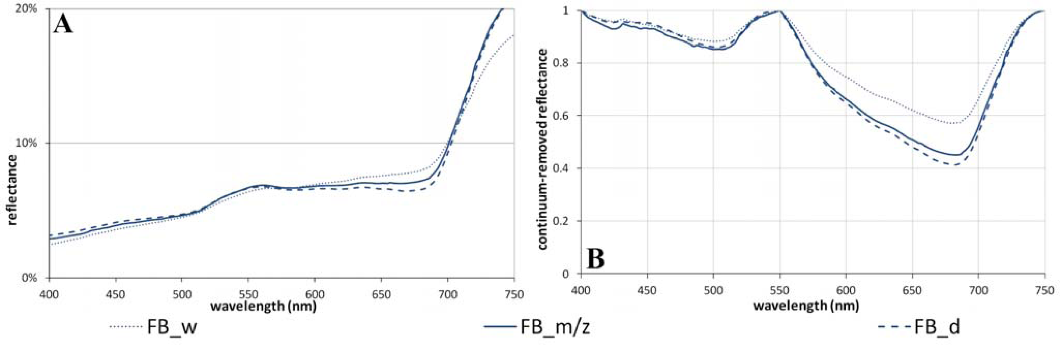
3.4. The Soil Moisture Gradient at Franklin Bluffs (Subzone D)

The three Franklin Bluffs study sites are separated into dry (36 Vol% soil moisture), mesic (zonal) (48 Vol%) and wet (74 Vol%) moisture regimes. This local soil moisture gradient is also noticeable in the averaged vegetation heights (Table 2). Whereas the dry site (FB_d) has a mean vegetation height of 14 cm, this increases to 15 cm at the mesic site (FB_m/z) and to 30 cm at the wet site (FB_w). The overall percentage cover of vegetation (non-lichen) ranges from 90 to 95% across the sites due to the effect of nonsorted circles, which have centers that are mainly covered by soil crusts. There is also a change in the vegetation composition and structure. At the wet site, sedges forming the second height stratum become more dominant and cover 80% of the whole area with a maximum height of 40 cm. The mesic site has a percentage cover of the second stratum of 82%, and the dry site of 40%. At both sites sedges and shrubs are the main species in this stratum. Shrubs form the third vertical stratum at the mesic site with 5% cover and a maximum height of 40 cm, whereas at the dry site the cover increases to 20%, but the height decreases to 35 cm. An increase of standing dead material can be seen from the dry to the wet site.

In the VIS wavelength region, the dry site has a green reflectance peak and a distinctive reflectance minimum in the red around 680 nm (Figure 12A). The reflectance spectrum of the mesic site has a distinctive green reflectance peak, but the local reflectance maximum is in the red wavelength region of chlorophyll absorption. The spectrum of the wet site has a steady reflectance increase up to 680 nm with even lower chlorophyll absorption and has a hardly noticeable green reflectance peak.

All three sites have nearly the same reflectance values in the 300 nm wide VIS band (5.7% to 5.8%) (Table 3). The results of the relative absorption depth analysis show a minor separation of the sites along the soil moisture gradient in the blue region and a more distinct separation in the red region. The relative absorption depth in the blue spectrum increases from 0.37 at FB_d, 0.41 at FB_m/z, to 0.44 at FB_w. In the red wavelength region this trend is reversed, so the absorption depth decreases from 1.07 at FB_d, 0.98 at FB_m/z, to 0.72 at FB_w. In addition, the continuum removal technique shows no clear site separation along the gradient in the blue (400–550 nm) region (Figure 12B). The area of the blue continuum removed absorption feature is 9.9 at FB_d, 11.9 at FB_m/z and 9.2 at FB_w, and the maximum band depth at 500 nm is 0.14 for the dry, 0.15 for the mesic and 0.12 for the wet site. A better separation along the gradient appears for the red absorption feature from 550–750 nm. The area of the absorption feature increases from 49.4 at FB_w, 64.5 at FB_m/z to 68.2 at FB_d. Likewise, the maximum continuum removed band depths at 680 nm increase from 0.43 for the wet site, 0.55 for the mesic, to 0.59 for the dry site.

In the NIR wavelength region the wet site has reduced reflectance values compared with the zonal and dry sites (Figure 5). In the 350 nm wide NIR band comparison, the wet site has an average reflectance of 21.9%, the dry site of 23.7%, and the mesic site of 24.6%. This sequence also appears in the comparison of the maximum reflectance at 1,020 nm. The wet site has a maximum reflectance of 25.7%, which increases to 26.9% for the dry site and to 28.9% for the mesic site.

4. Discussion

4.1. Overview of Field Characterization and Spectral Properties along the Gradients

The average reflectance spectra of the nine Low Arctic sites as a group are distinctly different from spectra of dominant vegetation in other higher and denser growing biomes. All the tundra spectra have generally low reflectance values, probably due to a combination of low plant canopy heights (vegetation height 8–30 cm, maximum shrub heights up to 55 cm) and low cover of vascular plants, relatively high cover of moss and lichen species, high surface moisture conditions, high sun zenith angles causing extreme shadowing by the plants themselves, and the large amounts of standing dead plant material. The averaged NIR reflectance for the tundra sites never exceeded 31%. It is well known that the presence of water reduces the overall reflectance, where the vegetation cover is more open [79]. Therefore, at Deadhorse (DH_z with 70 Vol% moisture) and the Franklin Bluffs wet site (FB_w with 74 Vol% moisture), despite the relative high averaged height of the vegetation structure, the high surface moisture absorbs in the NIR, and the NIR reflectance is thereby reduced. The high sun zenith angles (always larger than 43°) in the tundra cause extreme shadowing even with low vegetation stature and micro-topography heights [80]. Shadows decrease the reflectance in the red and NIR wavelength regions [81]. This effect can be especially important in tussock tundra (subzone E). High percentage nadir-cover of moss and lichen in the understory (8%–64% in this study) reduces the reflectance in the NIR wavelength region (Figure 13). Lichens also reduce the reflectance in the green wavelength region (Figure 13). Standing dead material, commonly dead sedge leaves in tundra, leads to an increase in the reflectance in the red wavelength region due to reduced chlorophyll absorption [26,82].

Figure 13 shows reflectance targets of tundra vegetation communities and of endmember targets (plant functional types) related to Arctic vegetation of subzones D and E. Two reflectance spectra have been measured over biological soil crusts: a reflectance spectrum of “moss/lichen/liverwort mix” from Clark et al. [83] and from nonsorted circles. Both reflectance spectra show considerable absorption in orange to red wavelengths with the development of a red-edge in contrast to reflectance spectra of barren soil surfaces without the development of a red-edge structure. Reflectance spectra of shrubs show high NIR backscatter with a planar NIR reflectance plateau with only minor or no slope between the beginning and end of the NIR reflectance plateau. This can be seen in the reflectance spectra of erect dwarf shrubs of 25 cm height and prostrate dwarf shrubs of 17 cm height (Figure 13). Both reflectance targets are characterized by dense and planophil leave structures. In contrast, reflectance spectra from sedges (30 cm) and tussock (20 cm) show NIR reflectance plateaus with stronger slopes between the beginning and end of the NIR reflectance plateau that also characterizes all the reflectance spectra of the tundra sites (Table 3, delta value between 1,020 nm and 750 nm). Reflectance targets with sedges and tussock show erectophile vegetation structure as well as dead plant material. They are therefore producing less multiple backscattering in the NIR. The structural dependence on planophil and erectophil vegetation structures on the NIR reflectance has been described by Thenkabail et al. [78] for crops.

The climate, soils, geomorphology, and hydrology of a site influence the vegetation characteristics, resulting in differences in leaf area and pigment composition, vegetation biomass and height, cover of plant functional types and total vegetation cover. These influence the VIS and NIR wavelength regions of the reflectance spectra. Thus, although the reflectance spectra of the main plant functional types (e.g., erect dwarf shrub, prostrate dwarf shrub, sedge) show certain diagnostic reflectance and absorption features, in combination as a plant community representing an area at larger scale (average reflectance of the site) it is challenging to distinguish the sites by their spectral signatures (Figure 13). The spectra of the nine tundra vegetation communities examined are superficially similar in many respects, when examined in detail, they show distinct diagnostic features mainly in the pigment absorbing wavelength bands and the height of the NIR reflectance.

The main changes in the VIS and NIR region of the spectra along the zonal climate gradient are likely due to differences in biomass, average and maximum vegetation height, and species composition. Since all contributors are physically overlapping, more research would be needed to partition the contributors causally. However, vegetation height, shrub-cover, and biomass increase toward the south [42,54], causes higher pigment absorption in the blue and red bands and higher reflectance in the NIR bands. Site locations further north have greater cover of sedges, and are characterized by less leaf mass and fewer chlorophyll-rich shrubs. Together with higher cover of standing dead material (mostly sedges), this leads to an increase in the reflectance in the red and blue wavelength regions with no development of a green reflectance peak due to reduced leaf pigment absorption. The 5% difference in the NIR reflectance between the northernmost (Deadhorse) and southernmost (Happy Valley) zonal study site (Table 3) is most likely related to canopy structure changes along the climate gradient (taller more dense vegetation in the warmer summer climates to the south). This leads to greater multiple scattering and to higher reflectance values in the NIR. The very low NIR reflectance at Deadhorse is also due to the high surface moisture conditions (up to 70 Vol% soil moisture).

Mesic acidic and non-acidic tundra are at first sight physiognomically similar in that sedges and dwarf shrubs dominate both types, but the species composition and the relative ratios of the different plant functional types are quite distinct. The very different species composition of the acidic and non-acidic tundra is likely responsible for important spectral differences. For example, MAT has a much larger component of chlorophyll-rich deciduous shrubs and generally taller and more horizontally continuous cover of green vegetation; whereas MNT is generally less green, with more standing dead sedge leaves, much less cover of erect deciduous shrubs, and greater cover of soil crust and lichen-covered soil associated with abundant nonsorted circles. The prostrate evergreen dwarf shrub Dryas integrifolia, an abundant MNT plant, often has a large non-green component composed of dead leaves and stems. In addition, the most common mosses in MAT are acidic Sphagnum mosses, while the non-acidic moss Tomentypnum nitens is most common in MNT. Effects of changes in the dominant moss species on reflectance spectra have not yet been evaluated. However, the moss layer (L1) of MNT sites are characterized by non-greenish hues (5Y) of pure chroma (=10) in contrast to greenish hues (2.5GY) of pure chroma (=10) at MAT sites.

The results of the field spectroscopy support the separation of acidic and non-acidic tundra in the VIS reflectance spectrum. MAT sites have deeper chlorophyll absorption in the blue and red wavelength regions than the non-acidic sites. Moreover, the MNT sites have a greater percentage of nonsorted circles and lichen vegetated areas the further north they are [17], resulting in decreases in the absorption of blue and red radiation. A separation of MAT vs. MNT in the NIR wavelength region is possible, but the averaged reflectance spectra overlap at some study sites. In this study, the hill crest site at Happy Valley shows a relatively low NIR reflectance in comparison to the other two acidic Happy Valley sites. This somewhat drier site has a higher vegetation nadir-coverage of moss and lichen and a lower nadir-coverage of taller vegetation, which can reduce the reflectance in the NIR region and produce an NIR reflectance similar to the signature of a dry non-acidic site. However, the erect deciduous dwarf shrubs, which are taller and denser than the prostrate evergreen dwarf shrubs at the non-acidic sites, have a greater multiple scattering effect, and this leads to higher reflectance values in the NIR of MAT.

Differences in the lateral water fluxes and moisture regimes along the sites also have spectral impacts. The differences in the reflectance spectra along the toposequence gradient at Happy Valley can be mainly explained by the changes in cover and height of the dwarf-shrub layer, which is linked to lateral water flux from the hill crest to the footslope. There is also an increase in the cover of tussock sedges down the topographic gradient, matching findings from Stow et al. [77] and Walker & Lederer [84] along a toposequence at Imnavait Creek. The shrub cover in the third vertical stratum (L3) increases by 18% from the hill crest to the footslope, and the average vegetation height increases by 13 cm. This leads to a downslope increase of green leaf area and biomass, and therefore to higher NIR reflectance values. A clear separation in the NIR region of the three reflectance spectra is therefore possible. In the VIS region the reflectance spectra of all three sites overlap. Only in the spectral metrics of absorption depth and continuum removal analysis of the red wavelength region is a separation of all three sites possible. At 680 nm, the footslope site shows the deepest chlorophyll absorption, and the hill crest site shows the least absorption. The difference can be best seen in the area of the red absorption feature from 550–750 nm. The hill crest site is exposed to greater stress. Due to drier soil conditions, the percentage nadir-cover of moss and lichen vegetated areas is greater, and the nadir-coverage by green leaf area is less than the other sites, which can explain the reduced chlorophyll absorption in the VIS spectra.

The three sites along the soil moisture gradient at Franklin Bluffs show an even higher contrast of the spectral contribution by water (dry site 36 Vol% soil moisture and wet site 74 Vol%). The main difference along this gradient is the percentage cover of sedge and standing dead vegetation as well as changes in surface moisture. The high percentage cover of standing dead material at the wet site increases the reflectance in the red wavelengths bands, whereas the moist and dry sites are greener and show deeper chlorophyll absorption. This can be best seen in the spectral metrics of the continuum removal analysis of the red wavelength region, as there are only minor differences in the blue absorption band depths between the sites. The spectral behavior in the NIR region is mainly influenced by the soil moisture and mean vegetation height. The reduced NIR reflectance at the wet site results from the increased surface moisture content. The mesic and dry sites have nearly similar reflectance spectra at the shorter wavelengths of the NIR, but at the dry site there is a higher nadir-coverage of moss and lichen and lower contribution from taller vegetation layers, which reduces the NIR reflectance above 900 nm. For remote sensing applications the contribution from ponds and lakes will have an influence on the reflectance of tundra landscapes and on the NDVI [85].

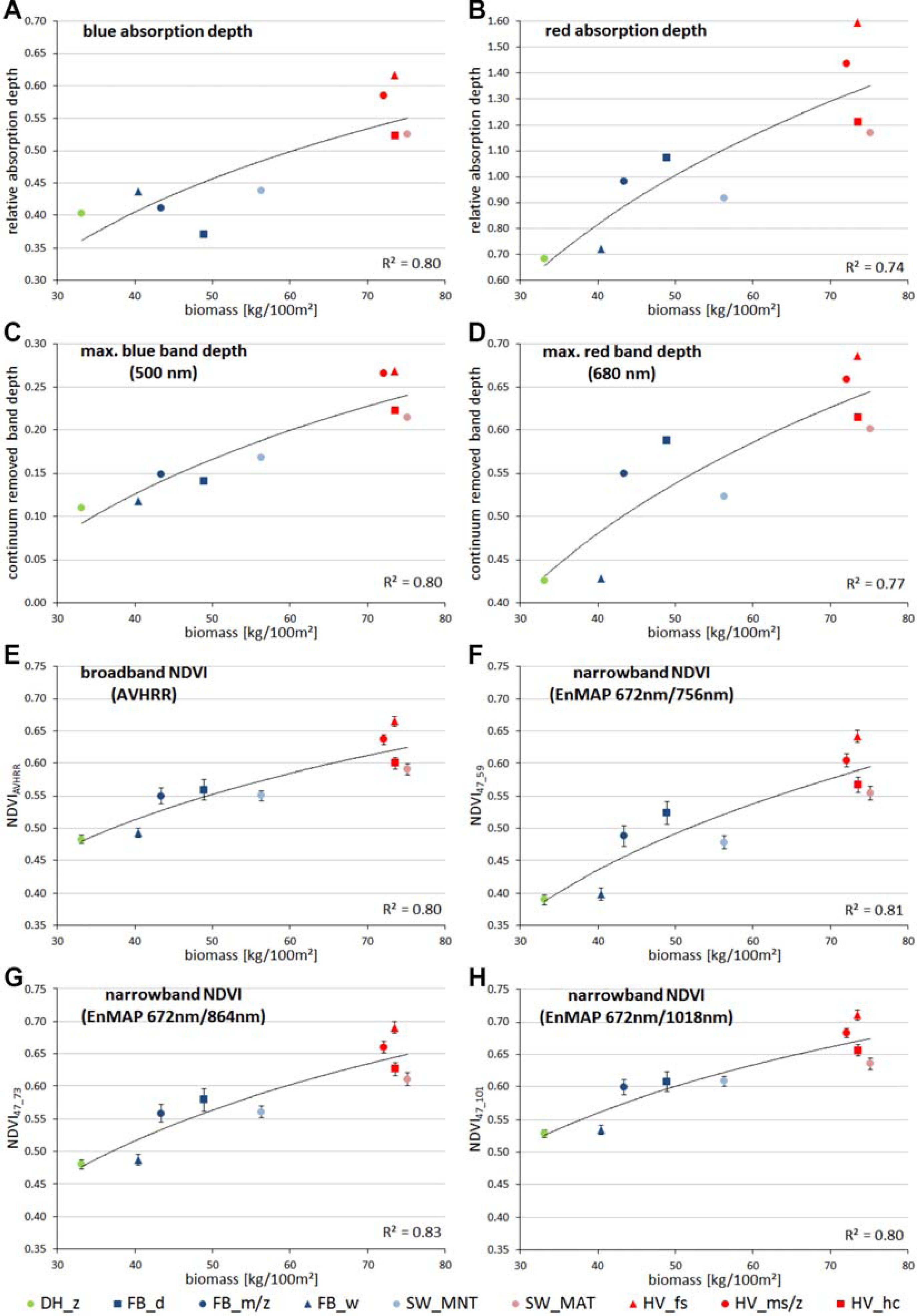
4.2. Performance of Spectral Metrics and Vegetation Indices

Since the continuum removal technique normalizes the absolute differences of local reflectance peaks in the green and NIR regions, it enhances the differences in absorption strength in the blue and red wavelength regions. The absorption-related metrics confirm the reduction in pigment absorption within the red and the blue wavelength regions along the climate gradient from south to north and from MAT to MNT. This can also be well seen in the regression analyses of the relative absorption depth and continuum removed maximum band depth in the blue and red wavelength regions with biomass (Figure 8).

Visually, MAT is much greener in mid-summer than MNT. Both have a dull brown appearance in early June, but, by July, the erect dwarf shrubs and tussock sedges of acidic tundra are fully leafed-out and mask the dead sedge leaves from the previous winter. The green-up in the non-acidic tundra is less striking, because there are fewer deciduous shrubs, and the new sedge leaves do not fully mask the standing dead leaves. Furthermore, there is much greater cover of soil crust and lichens on nonsorted circles, which are usually abundant in non-acidic tundra. The very distinct assignment of the dominant non-greenish hue (5Y) of pure chroma (=10) of the MNT sites in contrast to the dominant greenish hue (2.5GY) of pure chroma (=10) of the moss layer (L1) further supports the characterization that MAT sites are “greener”.

The partitioning of MAT and MNT using broadband and narrowband NDVIs in this study shows promising results. A broadband NDVI_AVHRR value of 0.58 and a narrowband NDVI_{47_59} value of 0.54 are the thresholds for separating these tundra systems in our study. The lower average NDVI values of MNT compared to MAT are mainly due to the lower quantities of shrub phytomass in MNT [15]. In non-acidic systems the phytomass is mainly composed of moss, which has a reduced NIR reflectance as well as less leaf mass with therefore reduced pigment absorption. The separation of acidic and non-acidic tundra via VIs and metrics of pigment absorption is important for remote sensing of Alaskan tundra, as this MAT/MNT threshold value can be extracted from the satellite image statistics.

That narrowband NDVIs may perform better than their broadband equivalent by setting one or both HNBs in the red and NIR to specific positions is already well known [32–34,78]. The main challenge is to find the right HNBs for an application within the large number of redundant bands provided by hyperspectral instruments [70]. Up to now, hyperspectral satellite and airborne data for arctic regions were limited. Therefore, ground-based hyperspectral measurements are a good alternative to determine HNBs for tundra applications. The three tested narrowband NDVIs showed similar good results in the regression analyses with biomass compared to the broadband NDVI. We assume that the performance of the broadband and narrowband NDVIs might not be fully linked to vegetation structure (i.e., NIR reflectance) due to low canopy height. The photosynthetic capacities of the tundra plant communities therefore seem to control the NDVI performance. This is illustrated by the regression relationships of biomass vs. NDVIs and biomass vs. absorption depths, respectively (Figure 8). The analyses indicate that the tundra sites characterized by sedges show less intense chlorophyll absorption due to more non-photosynthetically active biomass. The correlation of carotenoid absorption in the blue wavelengths with biomass (Figure 8A,C), therefore, shows a better performance than the correlation of chlorophyll absorption with biomass (Figure 8B,D). This differential and its influence on the NDVI facilitate the separation of MAT and MNT. Narrowband NDVIs, specifically the NDVI_{47_59} with the EnMAP NIR band 59 at 756 nm close to the red-edge, yield better separations of the two tundra vegetation types than the broadband NDVI. Imaging spectroscopy by new satellite systems such as EnMAP can be used to apply hyperspectral algorithms based on the narrow wavelength regions that show high separation potential between tundra communities. Narrowband methods using the spectral bands of pigment absorption around 500 nm for carotenoids and around 680 nm for chlorophyll show high potential.

5. Conclusions

This paper provides a ground-based hyperspectral characterization of the most important plant communities in the Alaskan Low Arctic tundra (subzones D and E) along important environmental gradients. As a group, the averaged reflectance spectra of all nine sites exhibit similar characteristic profiles that are typical for Low Arctic tundra (Figure 5). They show: (i) low maximum near-infrared (NIR) reflectance (maximum of 31% at 1,020 nm); (ii) weakly visible green reflectance peak or no local reflectance maximum in the visible spectrum; (iii) narrow “red-edge” region between the red and NIR wavelength regions (maximum 18% difference between red absorption minimum and NIR reflectance plateau); and (iv) no distinct NIR reflectance plateau (i.e., the “red-edge” bend does not finish in a plateau, instead the reflectance values steadily increase up to the maximum reflectance at around 1,020 nm). The explanation for these findings is that a generally low reflectance in the NIR as well as the green wavelength range and a low chlorophyll absorption in the red wavelength range occur due to a low vegetation height structure and low green leaf area of the vegetation. Moreover, nadir-coverage of standing dead sedges and woody plant material (dwarf shrubs) is generally high. These typical patterns make the reflectance spectra of low-growing tundra specific and distinguishable from other biomes, for example wetlands or local areas occupied by taller and denser growing shrubs.

This research also shows that spectral metrics follow the geoecological gradients. The reflectances of the NIR shoulder and NIR reflectance plateau are valuable information sources that separate the communities according to their biomass and vegetation structure. The spectral metrics of absorption depths and continuum removal technique reveal separation possibilities in the blue and red wavelength regions. The main spectro-radiometric findings are: (i) for the zonal gradient - there is more vegetation biomass, denser shrub cover and taller shrubs with denser leaf cover the further south along the North American Arctic Transect (NAAT). This leads to higher reflectance in the NIR wavelength region. (ii) Lower positions along toposequences and wetter sites along the soil moisture gradient show greater vegetation biomass due to higher moisture availability. However, this does not always lead to higher reflectance values in the NIR wavelength region. Vegetation height and surface wetness are two antagonists that may balance each other out with respect to the NIR reflectance. (iii) Moist acidic tundra (MAT) sites, when compared to moist non-acidic tundra (MNT) sites, have “greener” species (chlorophyll-rich deciduous shrubs and green-colored mosses), more continuous cover of green vegetation, and more leaf mass, which cause higher pigment absorption in the blue and red wavelength regions. (iv) MNT sites show relatively high reflectance in the red wavelength region, low absorption in the blue and red wavelength regions, and no distinct “green” reflectance. The contributing factors to low greenness are the abundance of standing dead sedge leaves, evergreen shrubs with larger non-green dead components (mainly Dryas integrifolia), higher percentage cover of soils covered by biological soil crusts, and abundance of brown-colored mosses (e.g., Tomentypnum nitens).

The hyperspectral field spectrometer analysis indicates the possibility of separating out MAT and MNT vegetation communities, which have not been previously separable in such a good way using broadband data. Moreover, hyperspectral data can potentially be used for color differentiation as well as investigation of differences in the shape and slope of the “red-edge” of MAT and MNT. Our investigation shows that additional types of field data to link to spectral metrics are needed. Future investigations should include evaluation of the amount of dead material per site as well as a more detailed assessment of the Munsell color of plant species and communities. In addition, time-series hyperspectral studies are needed through the growing season in combination with simultaneous studies of plant pigment concentrations in order to analyze the seasonal vegetation and color changes of tundra communities. Field spectroscopy is a useful method for obtaining hyperspectral ground data. This well-characterized spectral database of Low Arctic NAAT vegetation communities covers a wide range of geoecological parameters and serves as the basis for further investigation of spectral properties of arctic vegetation communities.

References

1. Bhatt, U.S.; Walker, D.A.; Raynolds, M.K.; Comiso, J.C.; Epstein, H.E.; Jia, G.; Gens, R.; Pinzon, J.E.; Tucker, C.J.; Tweedie, C.E.; et al. Circumpolar arctic tundra vegetation change is linked to sea ice decline. Earth Interact 2010, 14, 1–20. [Google Scholar]
2. Lawrence, D.M.; Slater, A.G.; Tomas, R.A.; Holland, M.M.; Deser, C. Accelerated Arctic land warming and permafrost degradation during rapid sea ice loss. Geophys. Res. Lett. 2008. [Google Scholar] [CrossRef]
3. Callaghan, T.V.; Tweedie, C.E.; Webber, P.J. Multi-decadal changes in tundra environments and ecosystems: The international polar year-back to the future project (IPY-BTF). AMBIO 2011, 40, 555–557. [Google Scholar]
4. Epstein, H.E.; Raynolds, M.K.; Walker, D.A.; Bhatt, U.S.; Tucker, C.J.; Pinzon, J.E. Dynamics of aboveground phytomass of the circumpolar Arctic tundra during the past three decades. Environ. Res. Lett 2012, 7, 15506. [Google Scholar]
5. Walker, M.D. From The Cover: Plant community responses to experimental warming across the tundra biome. Proc. Natl. Acad. Sci. USA 2006, 103, 1342–1346. [Google Scholar]
6. Winton, M. Amplified Arctic climate change: What does surface albedo feedback have to do with it? Geophys. Res. Lett 2006. [Google Scholar] [CrossRef]
7. Walker, D.A.; Bhatt, U.S.; Epstein, H.E.; Bieniek, P.; Comiso, J.; Frost, G.V.; Pinzon, J.; Raynolds, M.K.; Tucker, C.J. Changing arctic tundra vegetation biomass and greenness—State of the climate in 2011. Bull. Amer. Meteor. Soc 2012, 93, S138–S139. [Google Scholar]
8. Ulrich, M.; Grosse, G.; Chabrillat, S.; Schirrmeister, L. Spectral characterization of periglacial surfaces and geomorphological units in the Arctic Lena Delta using field spectrometry and remote sensing. Remote Sens. Environ 2009, 113, 1220–1235. [Google Scholar] [Green Version]
9. Olthof, I.; Fraser, R. Mapping northern land cover fractions using Landsat ETM+. Remote Sens. Environ 2007, 107, 496–509. [Google Scholar]
10. Stow, D.A.; Hope, A.; McGuire, D.; Verbyla, D.; Gamon, J.; Huemmrich, F.; Houston, S.; Racine, C.; Sturm, M.; Tape, K.; et al. Remote sensing of vegetation and land-cover change in arctic tundra ecosystems. Remote Sens. Environ 2004, 89, 281–308. [Google Scholar]
11. Raynolds, M.K.; Walker, D.A.; Epstein, H.E.; Pinzon, J.E.; Tucker, C.J. A new estimate of tundra-biome phytomass from trans-Arctic field data and AVHRR NDVI. Remote Sens. Lett 2012, 3, 403–411. [Google Scholar]
12. Vierling, L.A.; Deering, D.W.; Eck, T.F. Differences in arctic tundra vegetation type and phenology as seen using bidirectional radiometry in the early growing season. Remote Sens. Environ 1997, 60, 71–82. [Google Scholar]
13. Kääb, A. Remote sensing of permafrost-related problems and hazards. Permafrost. Periglacial. Pro 2008, 19, 107–136. [Google Scholar]
14. Laidler, G.; Treitz, P.; Atkinson, D. Remote sensing of Arctic vegetation: Relations between the NDVI, spatial resolution and vegetation cover on Boothia Peninsula, Nunavut. Arctic 2008, 61, 1–13. [Google Scholar]
15. Riedel, S.M.; Epstein, H.E.; Walker, D.A. Biotic controls over spectral reflectance of arctic tundra vegetation. Int. J. Remote Sens 2005, 26, 2391–2405. [Google Scholar]
16. Huemmrich, F.; Gamon, J.A.; Tweedie, C.; Oberbauer, S.F.; Kinoshita, G.; Houston, S.; Kuchy, A.; Hollister, R.D.; Kwon, H.; Mano, M.; et al. Remote sensing of tundra gross ecosystem productivity and light use efficiency under varying temperature and moisture conditions. Remote Sens. Environ 2010, 114, 481–489. [Google Scholar]
17. Hope, A.; Kimball, J.S.; Stow, D.A. The relationship between tussock tundra spectral reflectance properties and biomass and vegetation composition. Int. J. Remote Sens 1993, 14, 1861–1874. [Google Scholar]
18. Olthof, I.; Latifovic, R. Short-term response of arctic vegetation NDVI to temperature anomalies. Int. J. Remote Sens 2007, 28, 4823–4840. [Google Scholar]
19. Walker, D.A.; Epstein, H.E.; Jia, G.J.; Balser, A.; Copass, C.; Edwards, W.J.; Gould, W.A.; Hollingsworth, J.; Knudson, J.; Maier, H.A.; et al. Phytomass, LAI, and NDVI in northern Alaska: Relationships to summer warmth, soil pH, plant functional types, and extrapolation to the circumpolar Arctic. J. Geophys. Res. 2003. [Google Scholar] [CrossRef]
20. Horler, D.N.H.; Dockray, M.; Barber, J. The red edge of plant leaf reflectance. Int. J. Remote Sens 1983, 4, 273–288. [Google Scholar]
21. Elvidge, C.D. Vegetation Reflectance Features in AVIRIS Data. Proceedings of the Sixth Thematic Conference on Remote Sensing for Exploration Geology: Applications, Technology, Economics, Houston, TX, USA, 16–19 May 1988; pp. 169–182.
22. Barnsley, M.; Settle, J.; Cutter, M.; Lobb, D.; Teston, F. The PROBA/CHRIS mission: A low-cost smallsat for hyperspectral multiangle observations of the Earth surface and atmosphere. IEEE Trans. Geosci. Remote Sens 2004, 42, 1512–1520. [Google Scholar]
23. Pearlman, J.; Barry, P.; Segal, C.; Shepanski, J.; Beiso, D.; Carman, S. Hyperion, a space-based imaging spectrometer. IEEE Trans. Geosci. Remote Sens 2003, 41, 1160–1173. [Google Scholar]
24. Stuffler, T.; Kaufmann, C.; Hofer, S.; Förster, K.P.; Schreier, G.; Mueller, A.; Eckardt, A.; Bach, H.; Penné, B.; Benz, U.; et al. The EnMAP Hyperspectral Imager—An Advanced Optical Payload for Future Applications in Earth Observation Programmes: Bringing Space Closer to People. Proceedings of the 57th International AstronauticalFederation (IAF) Congress, Valencia, Spain, 2–6 October 2006; pp. 115–120.
25. Schaepman, M.E.; Ustin, S.L.; Plaza, A.J.; Painter, T.H.; Verrelst, J.; Liang, S. Earth system science related imaging spectroscopy—An assessment. Remote Sens. Environ 2009, 113, S123. [Google Scholar]
26. Asner, G.P. Biophysical and biochemical sources of variability in canopy reflectance. Remote Sens. Environ 1998, 64, 234–253. [Google Scholar]
27. Jakomulska, A.; Zagajewski, B.; Sobczak, M. Field Remote Sensing Techniques for Mountains Vegetation Investigation. Proceedings of the 3rd EARSeL workshop on Imaging Spectroscopy, Herrsching, Germany, 13–16 May 2003; pp. 580–596.
28. Gitelson, A.A.; Gritz, Y.; Merzlyak, M.N. Relationships between leaf chlorophyll content and spectral reflectance and algorithms for non-destructive chlorophyll assessment in higher plant leaves. J. Plant. Physiol 2003, 160, 271–282. [Google Scholar]
29. Gausman, H.W. Leaf reflectance of near-infrared. Photogramm. Eng. Remote Sensing 1974, 40, 183–191. [Google Scholar]
30. Richardson, A.J.; Wiegand, C.L. Distinguishing vegetation from soil background information: A gray mapping technique allows delineation of any Landsat scene into vegetative cover stages, degrees of soil brightness, and water. Photogramm. Eng. Remote Sensing 1977, 43, 1541–1552. [Google Scholar]
31. Thenkabail, P.S.; Smith, R.B.; de Pauw, E. Hyperspectral vegetation indices and their relationships with agricultural crop characteristics. Remote Sens. Environ 2000, 71, 158–182. [Google Scholar]
32. Roberts, D.; Roth, K.; Perroy, R. Hyperspectral Vegetation Indices. In Hyperspectral Remote Sensing of Vegetation; Thenkabail, P.S., Lyon, J.G., Huete, A., Eds.; CRC Press/Taylor and Francis Group: Boca Raton, FL, USA/London, UK/New York, NY, USA, 2011; pp. 309–328. [Google Scholar]
33. Elvidge, C.D.; Chen, Z. Comparison of broad-band and narrow-band red and near-infrared vegetation indices. Remote Sens. Environ 1995, 54, 38–48. [Google Scholar]
34. Thenkabail, P.; Lyon, J.; Huete, A. Advances in Hyperspectral Remote Sensing of Vegetation and Agricultural Croplands. In Hyperspectral Remote Sensing of Vegetation; Thenkabail, P.S., Lyon, J.G., Huete, A., Eds.; CRC Press/Taylor and Francis Group: Boca Raton, FL, USA/London, UK/New York, NY, USA, 2011; pp. 3–36. [Google Scholar]
35. Walker, D.A.; Raynolds, M.K.; Daniëls, F.J.A.; Einarsson, E.; Elvebakk, A.; Gould, W.A.; Katenin, A.E.; Kholod, S.S.; Markon, C.J.; Melnikov, E.S.; et al. The Circumpolar arctic vegetation map. J. Veg. Sci 2005, 16, 267–282. [Google Scholar]
36. Kuparuk River Basin Vegetation: Vegetation Classification for the Kuparuk River Basin Vegetation Mapping Project; Alaska Geobotany Center: Fairbanks, AK, USA, 2010.
37. Walker, D.A.; Epstein, H.E.; Romanovsky, V.E.; Ping, C.L.; Michaelson, G.J.; Daanen, R.P.; Shur, Y.; Peterson, R.A.; Krantz, W.B.; Raynolds, M.K.; et al. Arctic patterned-ground ecosystems: A synthesis of field studies and models along a North American Arctic Transect. J. Geophys. Res. 2008. [Google Scholar] [CrossRef]
38. Buchhorn, M.; Schwieder, M. Expedition “EyeSight-NAAT-Alaska” 2012. In Expeditions to Permafrost 2012: “Alaskan North Slope/Itkillik”,“Thermokarst in Central Yakutia”, “EyeSight-NAAT-Alaska”; Alfred-Wegener-Inst. für Polar- und Meeresforschung: Bremerhaven, Germany, 2012; pp. 41–65. [Google Scholar]
39. Kade, A.; Walker, D.A.; Raynolds, M.K. Plant communities and soils in cryoturbated tundra along a bioclimate gradient in the Low Arctic, Alaska. Phytocoenologia 2005, 35, 761–820. [Google Scholar]
40. Vonlanthen, C.M.; Walker, D.A.; Raynolds, M.K.; Kade, A.; Kuss, P.; Daniëls, F.J.A.; Matveyeva, N.V. Patterned-ground plant communities along a bioclimate gradient in the high arctic, Canada. Phytocoenologia 2008, 38, 23–63. [Google Scholar]
41. Walker, D.A.; Epstein, H.E.; Welker, J.M. Introduction to special section on biocomplexity of arctic tundra ecosystems. J. Geophys. Res 2008. [Google Scholar] [CrossRef]
42. Walker, D.A.; Kuss, P.; Epstein, H.E.; Kade, A.N.; Vonlanthen, C.M.; Raynolds, M.K.; Daniëls, F.J. Vegetation of zonal patterned-ground ecosystems along the North America Arctic bioclimate gradient. Appl. Veg. Sci 2011, 14, 440–463. [Google Scholar]
43. Alaska Geobotany Center. North American Arctic Transect, Data Reports. 2013. Available online: http://www.geobotany.uaf.edu/naat/data (accessed on 6 February 2013).
44. Walker, D.A. Hierarchical subdivision of Arctic tundra based on vegetation response to climate, parent material and topography. Glob. Change. Biol 2000, 6, 19–34. [Google Scholar]
45. Razzhivin, V.Y. Zonation of Vegetation in the Russian Arctic. In The Species Concept in the High North: A Panarctic Flora Initiative; Nordal, I., Razzhivin, V.Y., Eds.; Norwegian Academy of Science and Letters: Oslo, Norway, 1999; pp. 113–130. [Google Scholar]
46. Walker, D.A.; Auerbach, N.A.; Bockheim, J.G.; Chapin, F.S.; Eugster, W.; King, J.Y.; McFadden, J.P.; Michaelson, G.J.; Nelson, F.E.; Oechel, W.C.; et al. Energy and trace-gas fluxes across a soil pH boundary in the Arctic. Nature 1998, 394, 469–472. [Google Scholar]
47. Zhang, T.; Osterkamp, T.E.; Stamnes, K. Some characteristics of the climate in Northern Alaska, USA. Arctic Alp. Res 1996, 28, 509–518. [Google Scholar]
48. Walker, M.D.; Walker, D.A.; Auerbach, N.A. Plant communities of a tussock tundra landscape in the brooks range Foothills, Alaska. J. Veg. Sci 1994, 5, 843–866. [Google Scholar]
49. Washburn, A.L. Geocryology: A Survey of Periglacial Processes and Environments; Wiley: New York, NY, USA, 1980. [Google Scholar]
50. De Molenaar, J.G. An Ecohydrological approach to floral and vegetational patterns in arctic landscape ecology. Arctic Alp. Res 1987, 19, 414–424. [Google Scholar]
51. Billings, W.D. Arctic and alpine vegetations: Similarities, differences, and susceptibility to disturbance. BioScience 1973, 23, 697–704. [Google Scholar]
52. Walker, D.A.; Auerbach, N.A.; Nettleton, T.K.; Gallant, A.; Murphy, S.M. Happy Valley Permanent Vegetation Plots; Institute of Arctic and Alpine Research: Boulder, CO, USA, 1997. [Google Scholar]
53. Epstein, H.E.; Walker, D.A.; Raynolds, M.K.; Jia, G.J.; Kelley, A.M. Phytomass patterns across a temperature gradient of the North American arctic tundra. J. Geophys. Res. 2008. [Google Scholar] [CrossRef]
54. Raynolds, M.K.; Walker, D.A.; Munger, C.A.; Vonlanthen, C.M.; Kade, A.N. A map analysis of patterned-ground along a North American arctic transect. J. Geophys. Res 2008, 113, 1–18. [Google Scholar]
55. Walker, D.A.; Epstein, H.E.; Raynolds, M.K.; Kuss, P.; Kopecky, M.A.; Frost, G.V.; Daniëls, F.J.A.; Leibman, M.O.; Moskalenko, N.G.; Matyshak, G.V.; et al. Environment, vegetation and greenness (NDVI) along the North America and Eurasia arctic transects. Environ. Res. Lett 2012, 7, 15504. [Google Scholar]
56. Dierschke, H. Pflanzensoziologie: Grundlagen und Methoden: 55 Tabellen; Ulmer: Stuttgart, Germany, 1994. [Google Scholar]
57. Kuehni, R.G. The early development of the Munsell system. Color Res. Appl 2002, 27, 20–27. [Google Scholar]
58. Spectra Vista Corporation. GER 1500—User manual: Revision 3.8; Spectra Vista Corporation: Poughkeepsie, NY, USA, 2009. [Google Scholar]
59. Milton, E.J. Review Article Principles of field spectroscopy. Int. J. Remote Sens 1987, 8, 1807–1827. [Google Scholar]
60. Milton, E.J.; Schaepman, M.E.; Anderson, K.; Kneubühler, M.; Fox, N. Progress in field spectroscopy: Imaging spectroscopy special issue. Remote Sens. Environ 2009, 113, S92–S109. [Google Scholar]
61. Schopfer, J.; Dangel, S.; Kneubühler, M.; Itten, K.I. The improved dual-view field goniometer system FIGOS. Sensors 2008, 8, 5120–5140. [Google Scholar]
62. Suomalainen, J.; Hakala, T.; Peltoniemi, J.; Puttonen, E. Polarised multiangular reflectance measurements using the finnish geodetic institute field goniospectrometer. Sensors 2009, 9, 3891–3907. [Google Scholar]
63. Crowley, J.K.; Brickey, D.W.; Rowan, L.C. Airborne imaging spectrometer data of the Ruby Mountains, Montana: Mineral discrimination using relative absorption band-depth images. Remote Sens. Environ 1989, 29, 121–134. [Google Scholar]
64. Clark, R.N.; Roush, T.L. Reflectance spectroscopy: Quantitative analysis techniques for remote sensing applications. J. Geophys. Res 1984, 89, 6329–6340. [Google Scholar]
65. Kokaly, R.F.; Clark, R.N. Spectroscopic determination of leaf biochemistry using band-depth analysis of absorption features and stepwise multiple linear regression. Remote Sens. Environ 1999, 67, 267–287. [Google Scholar]
66. Mutanga, O.; Skidmore, A.; Prins, H. Predicting in situ pasture quality in the Kruger National Park, South Africa, using continuum-removed absorption features. Remote Sens. Environ 2004, 89, 393–408. [Google Scholar]
67. Schmidt, K.S.; Skidmore, A. Spectral discrimination of vegetation types in a coastal wetland. Remote Sens. Environ 2003, 85, 92–108. [Google Scholar]
68. Romney, A.K.; Fulton, J.T. Transforming reflectance spectra into Munsell color space by using prime colors. Proc. Natl. Acad. Sci. USA 2006, 103, 15698–15703. [Google Scholar]
69. Braun, A.C.; Weidner, U.; Hinz, S. Support vector machines for vegetation classification—A revision (in German). Photogramm. Fernerkund. Geoinf 2010, 2010, 273–281. [Google Scholar]
70. Thenkabail, P.S.; Mariotto, I.; Gumma, M.K.; Middleton, E.M.; Landis, D.R.; Huemmrich, K.F. Selection of Hyperspectral Narrowbands (HNBs) and Composition of Hyperspectral Twoband Vegetation Indices (HVIs) for biophysical characterization and discrimination of crop types using field reflectance and hyperion/EO-1 data. IEEE J. Sel. Top. Appl. Earth Obs. Remote Sens 2013, 6, 427–439. [Google Scholar]
71. Buddenbaum, H.; Stern, O.; Stellmes, M.; Stoffels, J.; Pueschel, P.; Hill, J.; Werner, W. Field imaging spectroscopy of beech seedlings under dryness stress. Remote Sens 2012, 4, 3721–3740. [Google Scholar]
72. Schlerf, M.; Atzberger, C.; Hill, J. Remote sensing of forest biophysical variables using HyMap imaging spectrometer data. Remote Sens. Environ 2005, 95, 177–194. [Google Scholar]
73. Buddenbaum, H.; Püschel, P. SpInMine (Spectral Index Data Mining Tool): Manual for Application: SpInMine (1.0); University of Trier: Trier, Germany, 2012. [Google Scholar]
74. Held, M.; Jakimow, B.; Rabe, A.; van der Linden, S.; Wirth, F.; Hostert, P. EnMAP-Box Manual: Version 1.4; Humboldt-Universität zu Berlin: Berlin, Germany, 2012. [Google Scholar]
75. Rouse, J.W.; Haas, R.H.; Schell, J.A.; Deering, D.W. Monitoring Vegetation Systems in the Great Plains with ERTS. Proceedings of the Third ERTS Symposium, Washington, DC, USA, 10–14 December 1973; pp. 309–317.
76. Tucker, C.J. Red and photographic infrared linear combinations for monitoring vegetation. Remote Sens. Environ 1979, 8, 127–150. [Google Scholar]
77. Stow, D.A.; Burns, B.H.; Hope, A. Spectral, spatial and temporal characteristics of Arctic tundra reflectance. Int. J. Remote Sens 1993, 14, 2445–2462. [Google Scholar]
78. Thenkabail, P.S.; Smith, R.B.; de Pauw, E. Evaluation of narrowband and broadband vegetation indices for determining optimal hyperspectral wavebands for agricultural crop characterization. Photogramm. Eng. Remote Sensing 2002, 68, 607–621. [Google Scholar]
79. Weidong, L.; Baret, F.; Xingfa, G.; Qingxi, T.; Lanfen, Z.; Bing, Z. Relating soil surface moisture to reflectance. Remote Sens. Environ 2002, 81, 238–246. [Google Scholar]
80. McGuffie, K.; Henderson-Sellers, A. Technical note. Illustration of the influence of shadowing on high latitude information derived from satellite imagery. Int. J. Remote Sens 1986, 7, 1359–1365. [Google Scholar]
81. Ranson, K.; T. Daughtry, C. Scene Shadow Effects on Multispectral Response. IEEE Trans. Geosci. Remote Sens. 1987, GE-25, 502–509. [Google Scholar]
82. Tucker, C.J. Spectral estimation of grass canopy variables. Remote Sens. Environ 1977, 6, 11–26. [Google Scholar]
83. Clark, R.N.; Swayze, G.A.; Wise, R.; Livo, E.; Hoefen, T.; Kokaly, R.; Sutley, S.J. USGS Digital Spectral Library Splib06a. 2007. Available online: http://speclab.cr.usgs.gov/spectral.lib06 (accessed on 6 February 2013).
84. Walker, D.A.; Lederer, N.D. Toposequence Study: Site Factors, Soil Physical and Chemical Properties and Plant Species Cover; Department of Energy, R4D Program Report, Institute of Arctic and Alpine Research: Boulder, CO, USA, 1987. [Google Scholar]
85. Muster, S.; Heim, B.; Abnizova, A.; Boike, J. Water body distributions across scales: A remote sensing based comparison of three arctic tundrawetlands. Remote Sens 2013, 5, 1498–1523. [Google Scholar]
Figure 1. (A) The Arctic bioclimate subzones of the Circumpolar Arctic Vegetation Map [35]. (B) Low Arctic part of the NAAT with the study locations Happy Valley, Sagwon, Franklin Bluffs, and Deadhorse. The map is based on the Kuparuk River Basin Vegetation map [36], which is derived from a Landsat mosaic.Note: The blue rectangle in (A) marks Alaska.
Remotesensing 05 03971f1
Figure 2. The nine study sites in relation to environmental gradients and zones concept (zonal climate, soil pH, soil moisture, and toposequence/hillslope) along the Low Arctic part of the NAAT.Note: Border color and texture are specific for each study site and will be used in all figures in order to distinguish between the sites.
Remotesensing 05 03971f2
Figure 3. Study sites along the NAAT and the main site characteristics [54,55]. Legend: LL: geographic coordinate (Latitude/Longitude); C: code for test site; SZ: bioclimatic subzone; TG: topography; VT: vegetation type; LFD: life form description.
Remotesensing 05 03971f3
Figure 4. Map of R2 values of hyperspectral two-band vegetation indices (HTBVI) of all possible simulated EnMAP band combinations correlated with biomass.Note: The graphs below and left of the 2D-correlogram contain the mean reflectance of all nine NAAT sites.
Remotesensing 05 03971f4
Figure 5. Diagnostic mean reflectance spectra of all nine study sites showing the general spectral characteristics of Alaskan Low Arctic tundra communities along the NAAT.Note: Naming and coloring of the reflectance spectra follow the concept shown in Figure 2.
Remotesensing 05 03971f5
Figure 6. Hyperspectral reflectance spectra of the study sites (grey lines: reflectance spectra of each quadrat; red line: averaged reflectance spectra representing the arctic tundra vegetation community of the study site; blue area: standard deviation of spectral signature).Note: The x-axis of the diagrams shows the wavelength in nm, and the y-axis shows the reflectance.
Remotesensing 05 03971f6
Figure 7. Spectral characteristics along the zonal climate gradient of the NAAT. Comparison of (A) the averaged reflectance spectra in the visible (400–700 nm), and (B) the continuum-removed absorption features in the blue (400–550 nm) and red (550 nm–750 nm) wavelength regions.Note: Naming and coloring of the reflectance spectra follow the concept shown in Figure 2.
Remotesensing 05 03971f7
Figure 8. Spectral metrics of the study sites as a function of biomass. (A) Relative blue absorption depth vs. biomass; (B) Relative red absorption depth vs. biomass; (C) Continuum removed maximum blue band depth vs. biomass; (D) Continuum removed maximum red band depth vs. biomass. Correlation between (E) broadband NDVI with biomass compared with three (FH) narrowband NDVIs with biomass.
Remotesensing 05 03971f8
Figure 9. Spectral characteristics of the plant communities on acidic and non-acidic soils (soil pH zones). Comparison of (A) the averaged reflectance spectra in the visible (400–700 nm), and (B) the continuum-removed absorption features in the blue (400–550 nm) and red (550–750 nm) wavelength regions.Note: All spectra of the sites belonging to acidic or non-acidic soils have been averaged and are shown with ±1 standard derivation.
Remotesensing 05 03971f9
Figure 10. (A) Histogram of the probability distribution of the broadband NDVIAVHRR (left) and narrowband NDVI47_59 (right) values of each quadrat, and (B) polynomial trends of the broadband NDVIAVHRR (left) and narrowband NDVI47_59 (right) distributions with a separation value (black dotted line) for acidic and non-acidic tundra.Note: Naming and coloring of the reflectance spectra follow the concept shown in Figure 2.
Remotesensing 05 03971f10
Figure 11. Spectral characteristics of the toposequence gradient at the Happy Valley study location. Comparison of (A) the averaged reflectance spectra in the visible (400–700 nm), and (B) the continuum-removed absorption features in the blue (400–550 nm) and red (550–750 nm) wavelength regions.Note: Naming and coloring of the reflectance spectra follow the concept shown in Figure 2.
Remotesensing 05 03971f11
Figure 12. Spectral characteristics of the soil moisture gradient at the Franklin Bluffs study location. Comparison of (A) the averaged reflectance spectra in the visible (400–700 nm), and (B) the continuum-removed absorption features in the blue (400–550 nm) and red (550–750 nm) wavelength regions.Note: Naming and coloring of the reflectance spectra follow the concept shown in Figure 2.
Remotesensing 05 03971f12
Figure 13. Reflectance spectra of the main plant functional types forming the plant communities of the Low Arctic portion of the NAAT.Note: For comparative purposes the mean reflectance spectra (plant community representation) of the zonal sites at Happy Valley, Franklin Bluffs and Deadhorse have been included. The reflectance spectrum of the “moss/lichen/liverwort mix” is retrieved from Clark et al. [83].
Remotesensing 05 03971f13