Correlation between Synthetic Aperture Radar Surface Winds and Deep Water Velocity in the Amundsen Sea, Antarctica

Abstract

The recent observed thinning of the glacier ice shelves in the Amundsen Sea (Antarctica) has been attributed to warm deep currents, possibly induced by along-coast winds in the vicinity of the glacial ice sheet. Here, high resolution maps of wind fields derived from Synthetic Aperture Radar (SAR) data have been studied and correlated with subsurface measurements of the deep water velocities in the Amundsen Sea area. Focus is on periods with low ice coverage in 2010 and 2011. In 2010, which had comparatively low ice coverage, the results indicate a more rapid response to wind forcing in the deep currents than in 2011. The SAR wind speed maps have better spatial resolution than available reanalysis data, and higher maximum correlation was obtained with SAR data than with reanalysis data despite the lower temporal resolution. The maximum correlation was R = 0.71, in a direction that is consistent with wind-driven Ekman theory. This is significantly larger than in previous studies. The larger correlation could be due to the better spatial resolution or the restriction to months with minimum ice coverage. The results indicate that SAR is a useful complement to infer the subsurface variability of the ocean circulation in remote areas in polar oceans.

1. Introduction

The Amundsen Sea is a seasonally ice-covered shelf sea on the West Coast of Antarctica. The ice shelves in the Amundsen Sea drain the West Antarctic Ice Sheet and have recently been observed to be thinning rapidly [1–4]. The main reason for their decline appears to be flow of warm dense water onto the shelf, channeled by bathymetric troughs leading to the deep inner basins. This has been observed on the Marguerite Trough [5–7] and on the Amundsen Shelf [8–10]. Model studies [11,12] indicate that the on-shelf flow of warm dense water is forced by along-shelf (i.e., eastward in the Amundsen Sea) winds. Field studies in the Amundsen Sea [13] indicate that eastward winds along the shelf break force a deep current toward the ice shelves in the submarine trough. Such a response is in accordance with standard wind-driven Ekman theory [14]: Because of the Earth’s rotation, the wind forces a surface flow directed to the left of the wind direction in the Southern Hemisphere (see Figure 1). Hence, eastward winds drive a northward Ekman transport in the surface layer, i.e., the top 20 m. In order to compensate for that flow a return current in the deeper water is induced which the mooring measures (Figure 1).

Synthetic Aperture Radar (SAR) images of the ocean surface have been used to produce maps of wind fields with high resolution at offshore areas worldwide (e.g., [15,16]). These instantaneous measurements of the wind field complements the reanalysis products that are averaged in space at a coarser resolution. In this work the impact of surface winds on deep currents in the Amundsen Sea is examined. Fields of the zonal wind component from ERA-interim [17] reanalysis data, from the European Center of Medium Range Weather Forecast (ECMWF) are used as well as wind speed retrieved from the Envisat Advanced SAR (ASAR) sensor. The wind data are correlated with current velocity from a moored current meter in the Amundsen Sea. The currents were measured in the lower half of the water column in a region where dense, relatively warm ocean water intrudes onto the continental shelf [9,13,18] in a deep trough that leads from the shelf break to the deep inner shelf basin (see Figure 2).

The mooring data set has previously been compared to ERA-interim analysis wind data [13], and found to have statistically significant correlation between along-trough current and zonal winds at the shelf and shelf-break. This is expected from Ekman theory (Figure 1), taking into account the fact that ocean currents are steered by bathymetry and hence expected to have the main flow direction along the deep trough at the site of the mooring. Although statistically significant, the maximum correlation was only about R = 0.41 [13], which means that there is more unexplained variance in the data than there is explained variance. The reason for the comparatively low correlation could be the low resolution of the ERA-interim data set or errors in the modeled data, possibly amplified during the ice-covered season. The wind data (both ERA interim and the SAR-derived) are less reliable when close to coastal or ice-covered areas [15–17]. The correlation between wind and currents is also likely smaller during the ice-covered season, since the sea-ice cover affects the momentum transfer between ocean and atmosphere. Here focus will be on the correlation for the time period with minimum ice cover.

2. Data

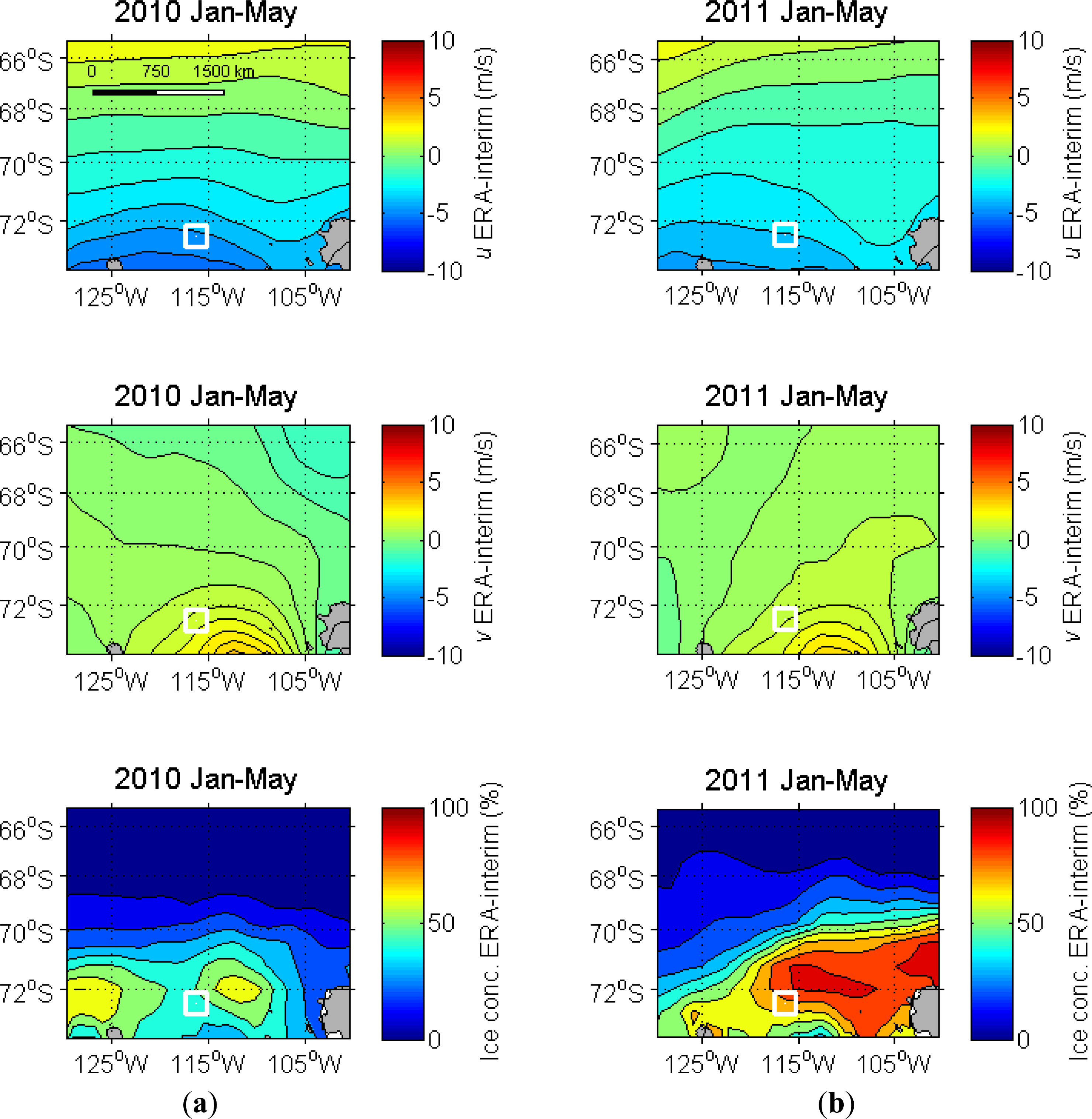
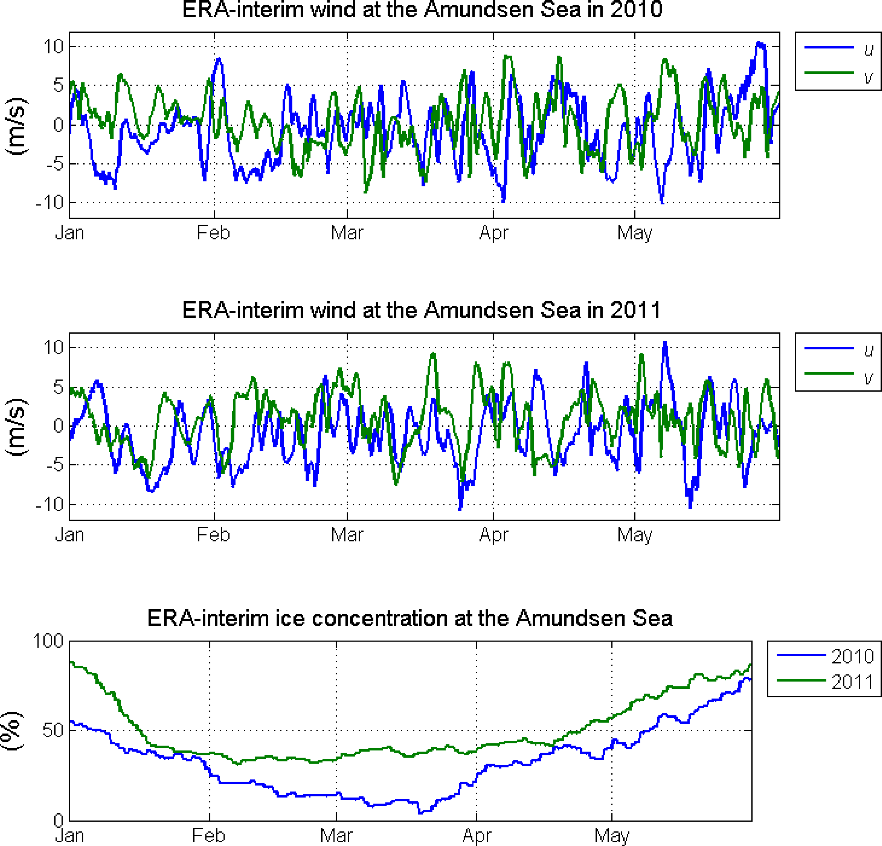
2.1. Wind and Ice Concentration from ERA-Interim

Figure 3 shows daily values of ERA-interim data averaged over the area 74°S to 65°S and 130°W to 100°W between January and May of 2010 and 2011 [17]. The zonal (u) and meridional (v) components of the 10 m wind are shown as well as the ice concentration. In general, both u and v components display a large variability with short periods of strong wind in both directions. The average ice concentration was higher in 2011 than in 2010, and both years had their minimum ice coverage between February and May.

Figure 4 shows the spatial variation of ERA-interim data averaged between January and May of 2010 and 2011, together with the mooring location. The temporal average over the area is close to zero, a consequence of the fact that the mean zonal wind changes direction between 74°S and 65°S. The open areas next to the coast (polynyas) can be noted in the ice concentration maps (Figure 4). These areas coincide with areas of strong meridional winds.

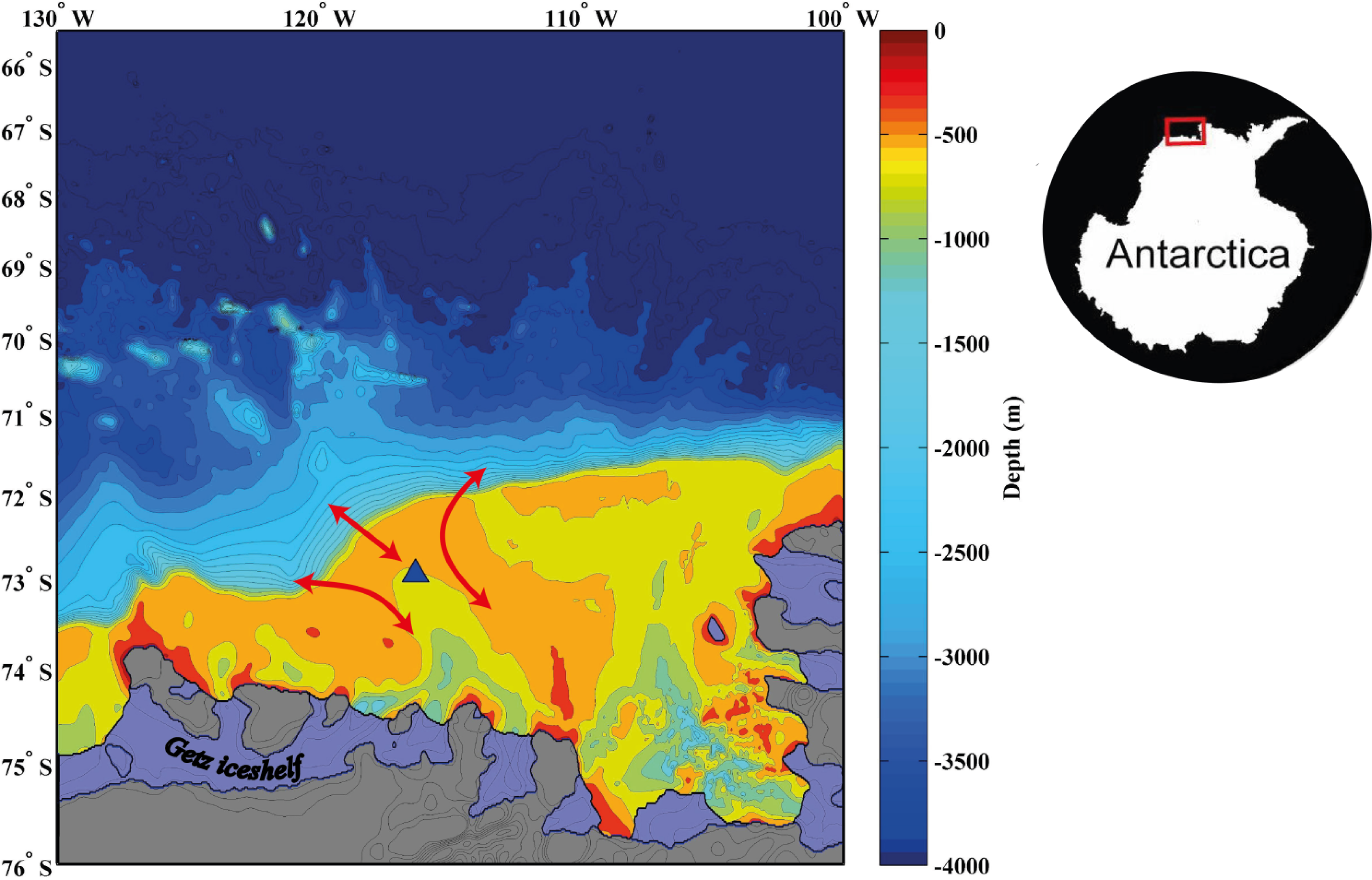
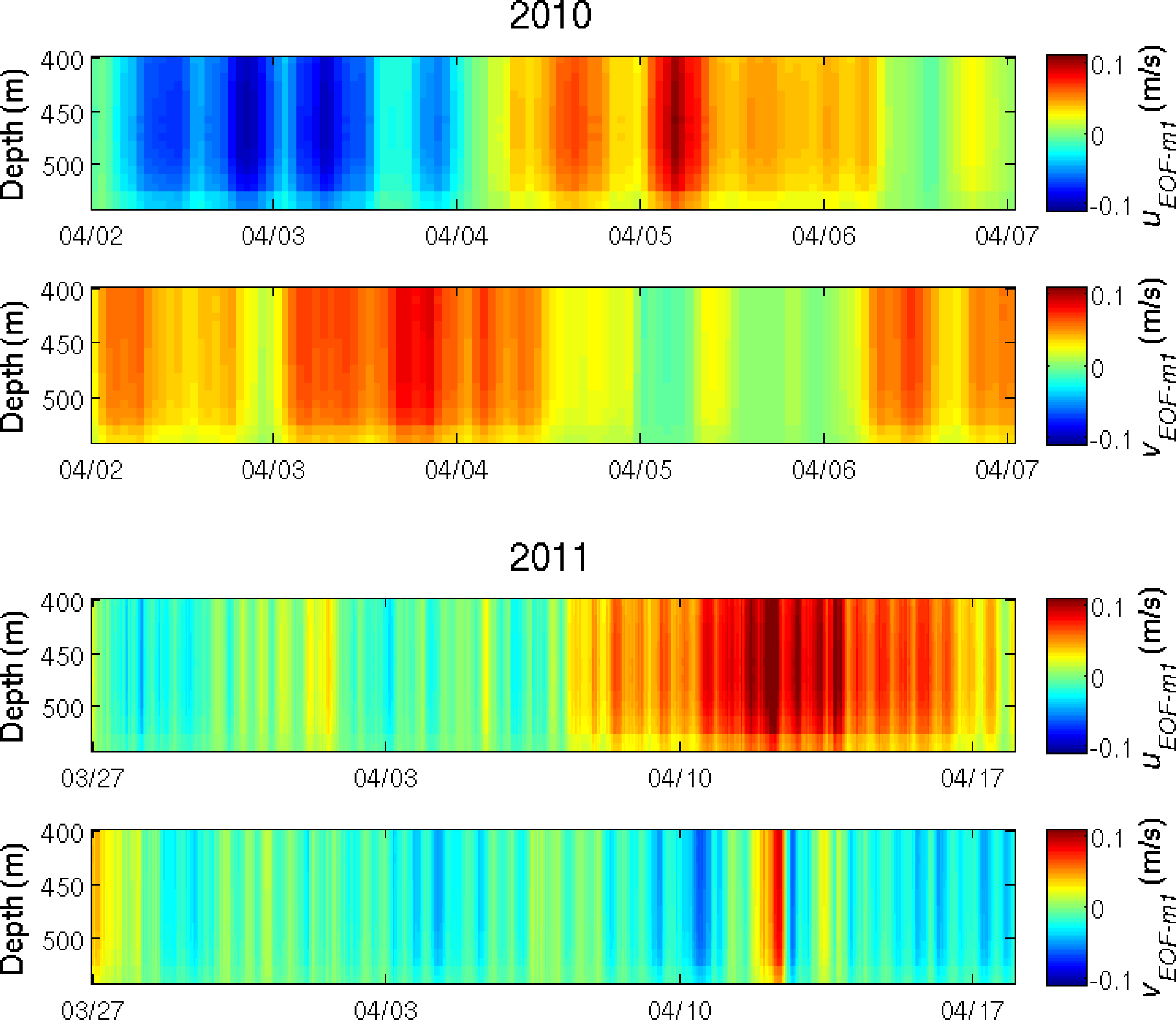
2.2. Deep Water Velocities from S1 Mooring

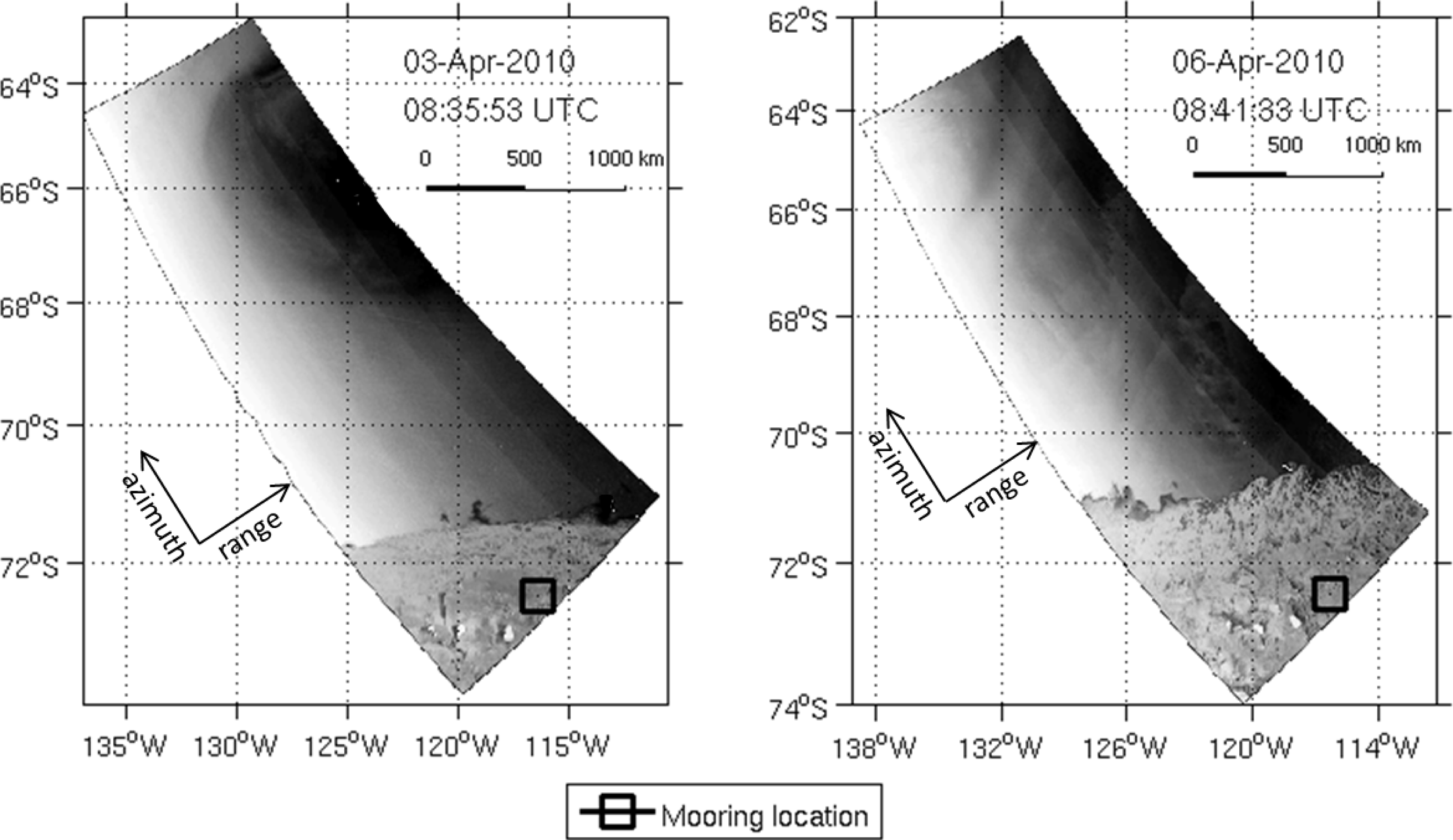
The mooring was deployed at 72.45°S and 116.34°W on 15 February 2010 and recovered on 1 March 2012 [13]. An upward-looking 150 kHz Acoustic Doppler Current Profiler (ADCP) was placed at the bottom, at 540 m depth. The ADCP was configured in narrow band mode for optimal range, using 8 m bins and 15 min ensembles of 25 pings each. The data were processed using the WinADCP software, filtering out data with error velocity exceeding 1.5 cm/s and beam correlation below 100. Daily averages of de-tided velocity (using the t_tide harmonic analysis, [19]) were decomposed into its Empirical Orthogonal Function (EOF; e.g., [20]) modes. The data above 360 m depth were removed due to large error velocity and/or low beam correlation. The first EOF mode (EOF1) accounted for over 90% of the total variance [13], and we focus here on only the EOF1 time series. The velocity components along (u_EOF–m1) and across (v_EOF–m1) the deep trough were studied by using a reference system with the u-axis parallel to the trough axis (v-axis rotated 42° clockwise from the North). The analyzed time period was limited to the time of minimum ice cover, i.e., the late summer and fall seasons of 2010 and 2011.

Figure 5 shows the daily averages of (u_EOF–m1) between 16 February and 31 May 2010 and between 8 February and 31 May 2011. The velocity is fluctuating on short (daily) time-scales. Two periods (black rectangles in Figure 5), one from 2 to 6 April 2010 and one from 27 March 27 to 17 April 2011, were singled out for closer scrutiny with SAR wind data. Hourly values for these periods are shown in Figure 6.

2.3. SAR Data

During 2010 the Amundsen Sea was regularly imaged by ascending passes of ASAR wide swath mode (WSM). For 2011, regular ASAR WSM images of the Amundsen Sea (ascending mode) were not available until 8 February. Available ASAR WSM data in the Amundsen Sea included 262 images acquired between 16 February and 31 May 2010, and 266 images acquired between 8 February and 31 May 2011.

SAR wind speed retrievals were computed for wind cells of 10 × 10 km² with the inversion of the CMOD-IFR2 [21], CMOD5 [22] and CMOD5.N [23] geophysical model functions (GMFs), using wind directions from ERA-interim analysis data. Although wind directions can be derived from the SAR image [16,24,25], we used ERA-interim model wind directions since the method only works when wind streaks [26] can be detected. The ERA-interim wind directions were averaged in time to match the SAR acquisition and spatially interpolated to the grid locations of the wind speed computation in Section 4.1.

Figure 7 shows two examples of the SAR images, after calibration and georeferencing. The brightness of the pixels is proportional to the normalized backscatter detected by the SAR sensor. The acquisition geometry of the SAR antenna, with a position approximately indicated by the coordinate axis with the azimuth and range vectors, produces a brightness gradient of the amplitude in the range direction. This is caused by the distance and illumination angle of the SAR sensor. The amplitude discontinuities in the range direction correspond to a bias introduced by mispointing of the SAR antenna [27]. The bias produces erroneous variations of the SAR wind speed retrievals but it is expected to be lower than the nominal error of 2 m/s.

3. Methodology

The time period January–May was chosen in order to have minimum sea ice cover. Since the ASAR WSM data have limited temporal coverage in the Amundsen Sea (only one to three images with partial coverage per day), the available images over a time period of two days were combined and averaged in time. Ice-covered areas were removed from both SAR and ERA interim data. An area was defined as covered with ice when the ice concentration (from ERA interim) was above 0.15 [28,29]. The ASAR wind values, originally computed for resolution cells of 10 × 10 km², were resampled and averaged over a grid with spacing of 0.2° in latitude and 0.5° in longitude. ERA-interim reanalysis wind data were averaged over two days in order to make the data sets comparable, and was used with its original grid spacing of 0.75° in both latitude and longitude.

In order to examine the correlation between the ASAR winds and the subsurface mooring velocity, correlation coefficients between the zonal surface wind field (u_wind) and the two EOF1 components (u_EOF–m1) and (v_EOF–m1) for the current velocity were calculated for each grid point and compared to the significance level. The large-lag significance test outlined in [30] were employed using confidence levels 95% and 99%. This method calculates the statistical significance based on the variability of the two time series and the lag.

4. Results and Discussion

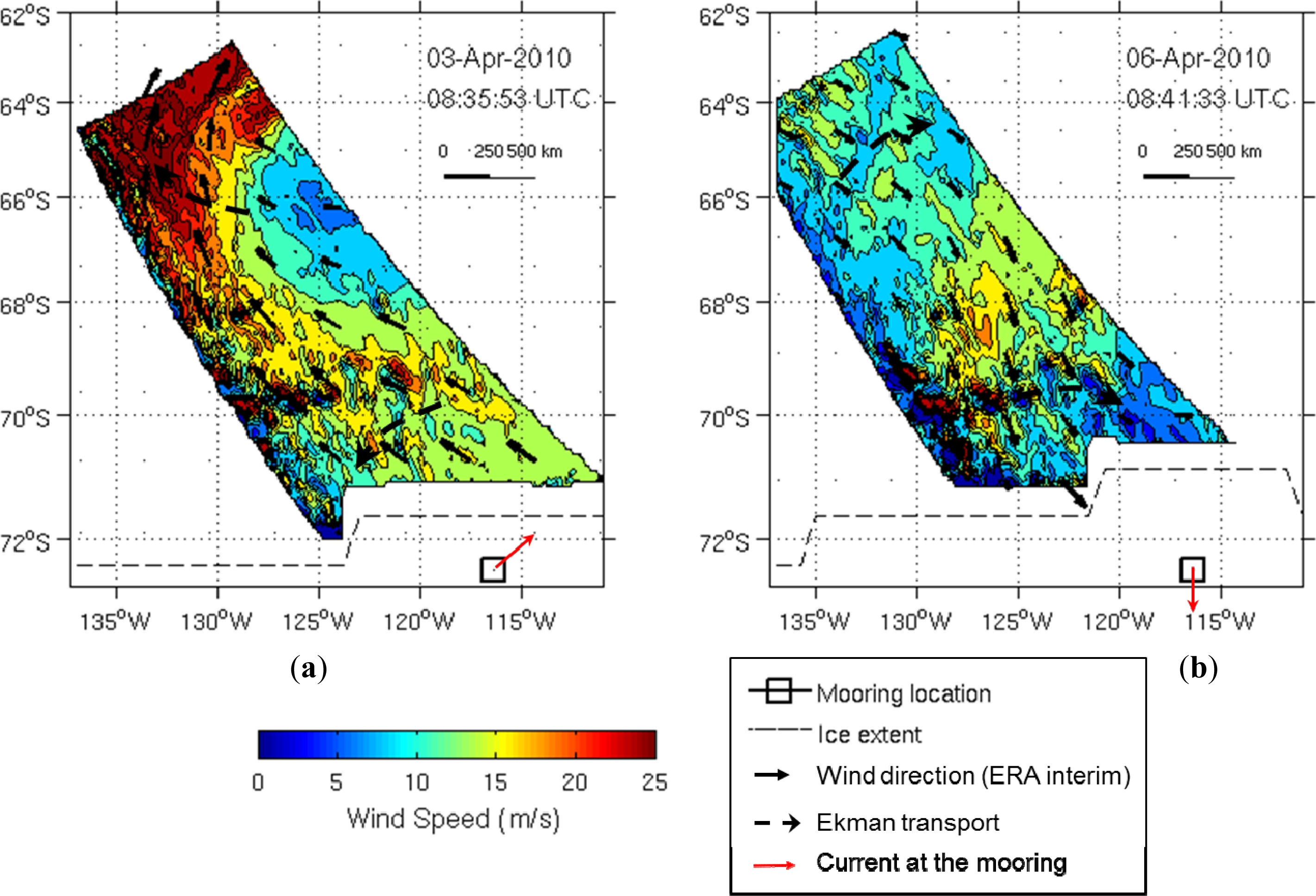
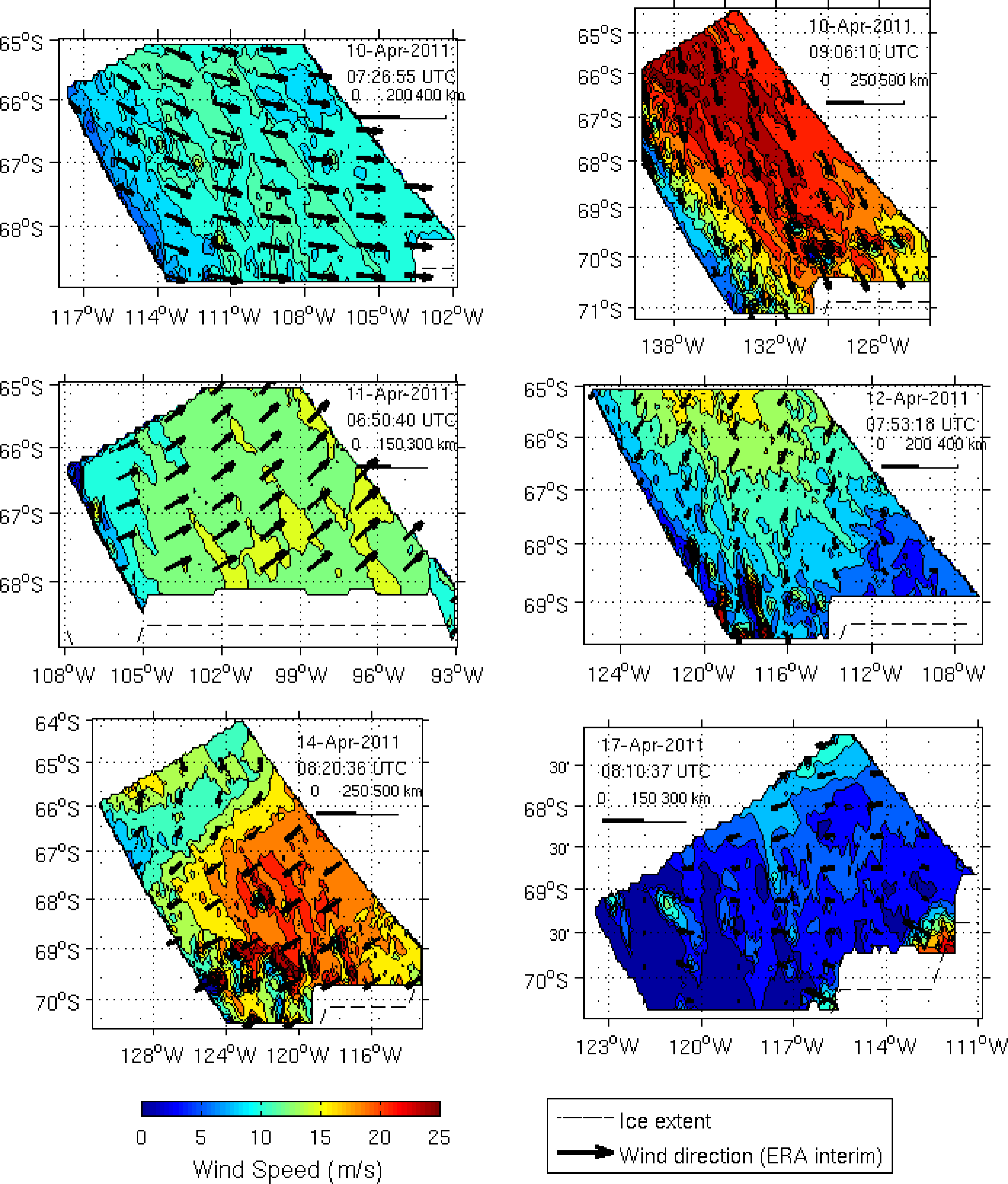
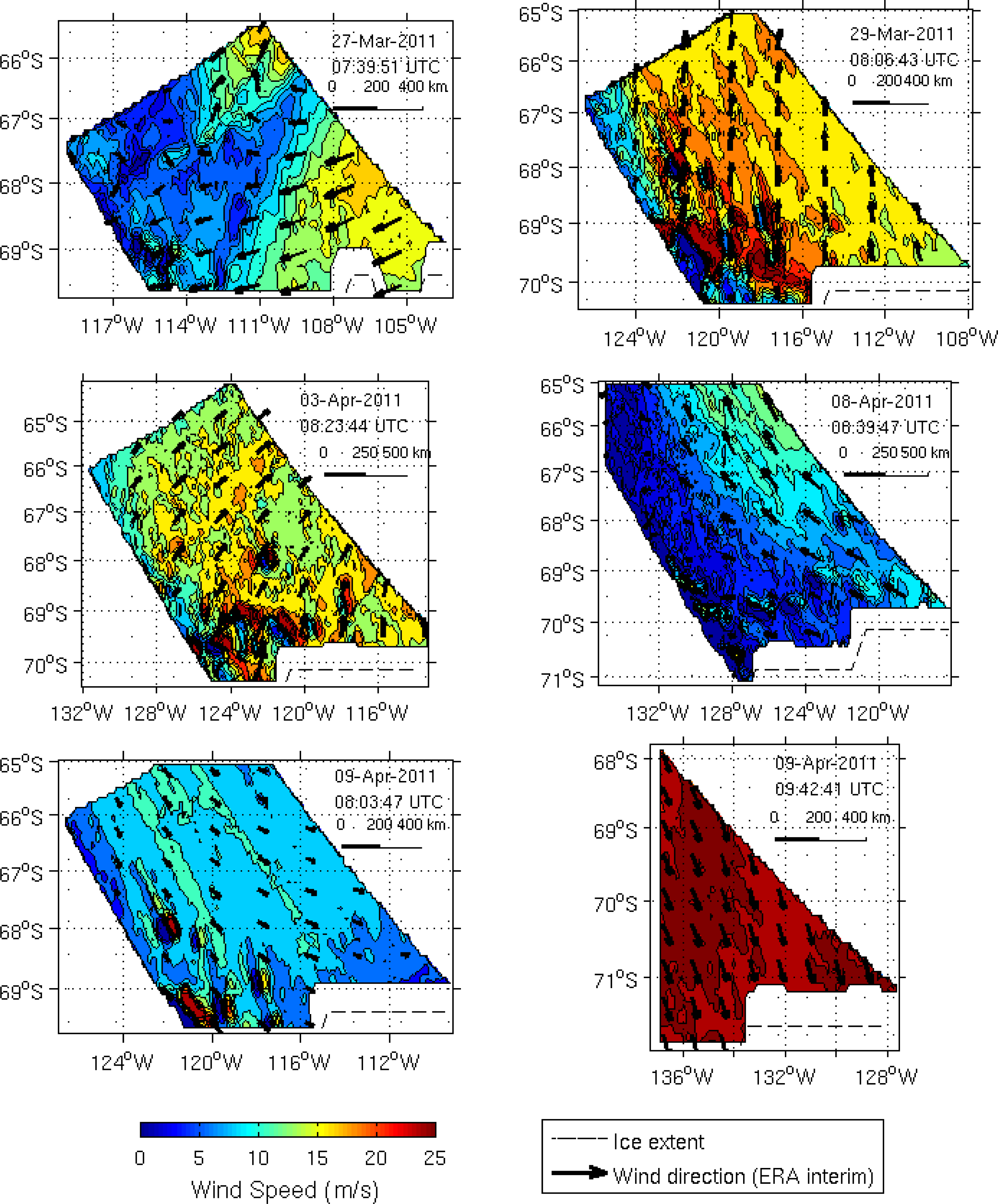
4.1. SAR Wind Maps

Figure 8 shows SAR wind speed retrievals (using CMOD-IFR2) from 2 to 6 April 2010 (see Figure 5), which includes the abrupt shift in direction of the deep current u_EOF–m1 on 4 April. On 3 April, there was a moderately strong south-easterly wind in the southern part of the region, and a strong southerly wind in the northern part. Such a wind field would induce a southwestward Ekman transport in the southern part and a strong westward Ekman transport further North (see dashed arrows in Figure 8). On 6 April, the wind had changed direction to northerly, which would induce an eastward Ekman transport (dashed arrows, Figure 8b). The observed current in the mooring is indicated as a red arrow, and it is oppositely directed to the Ekman transport on 3 April. On 6 April the deep current is southward. The recorded deep current can hence be the return flow from the Ekman transport (Figure 1), and the recorded switch in direction on 4 April could be caused by the wind shift at some time between 3 and 6 April.

The next example (Figure 9) is from 27 March to 17 April 2011. The current in the deep trough during this period first had low velocities with fluctuating direction, and then changed to a strong and persistent southward flow around 10 April. The wind observations between 27 March and 17 April first showed weak or moderate winds of fluctuating direction, that has changed to very strong north-westerly winds on 9 April persisting until 11 April. On 12 April the winds changed direction to easterly. According to Ekman theory, the mainly north-westerly winds between 9 and 11 April should cause a positive subsurface velocity in the deep trough, as was also observed in the mooring. However, the strongest current occurred on 13 April, a few days after the strongest wind. Also, the southward current continued a few days after the wind switched direction.

It is hypothesized that the possible delay of the wind effect on the current in the trough can be a consequence of the average strength of the wind and the extent of the ice sheet. Although the wind field changes direction it is possible that in ice-covered seas only strong persistent winds are able to affect the deep currents. It could also be that the presence of the sea ice gives a delayed response in the deep water column since it takes a while for the ice sheet to gain momentum.

Some of the wind maps (e.g., 3 April 2010, 6 April 2010, 29 March 2011, 3 April 2011, 9 April 2011 and 14 April 2011) display small clusters with high wind speeds. These clusters are attributed to signatures of rain cells in the SAR data [31], which cause rain-induced turbulence, modify the Bragg waves and thus affect the SAR wind speed retrieval. The wind speeds derived with CMOD-IFR2, CMOD5 and CMOD5.N GMFs did not show significant differences except in the locations associated with rain-cell signatures, where the CMOD5 and CMOD5.N wind speeds generally give larger variations than the ones from CMOD-IFR2. In all wind maps the ice covered areas have been excluded (see e.g., by comparing Figures 7 and 8) so the errors introduced by the presence of sea ice should be small. However, the discontinuities from the mispointing of the ASAR antenna (Section 2.3) produce artificial variations of the wind speed pattern observed in some of the wind maps (e.g., 6 April 2010, 29 March 2011, 9 April 2011, 10 April 2011 and 11 April 2011).

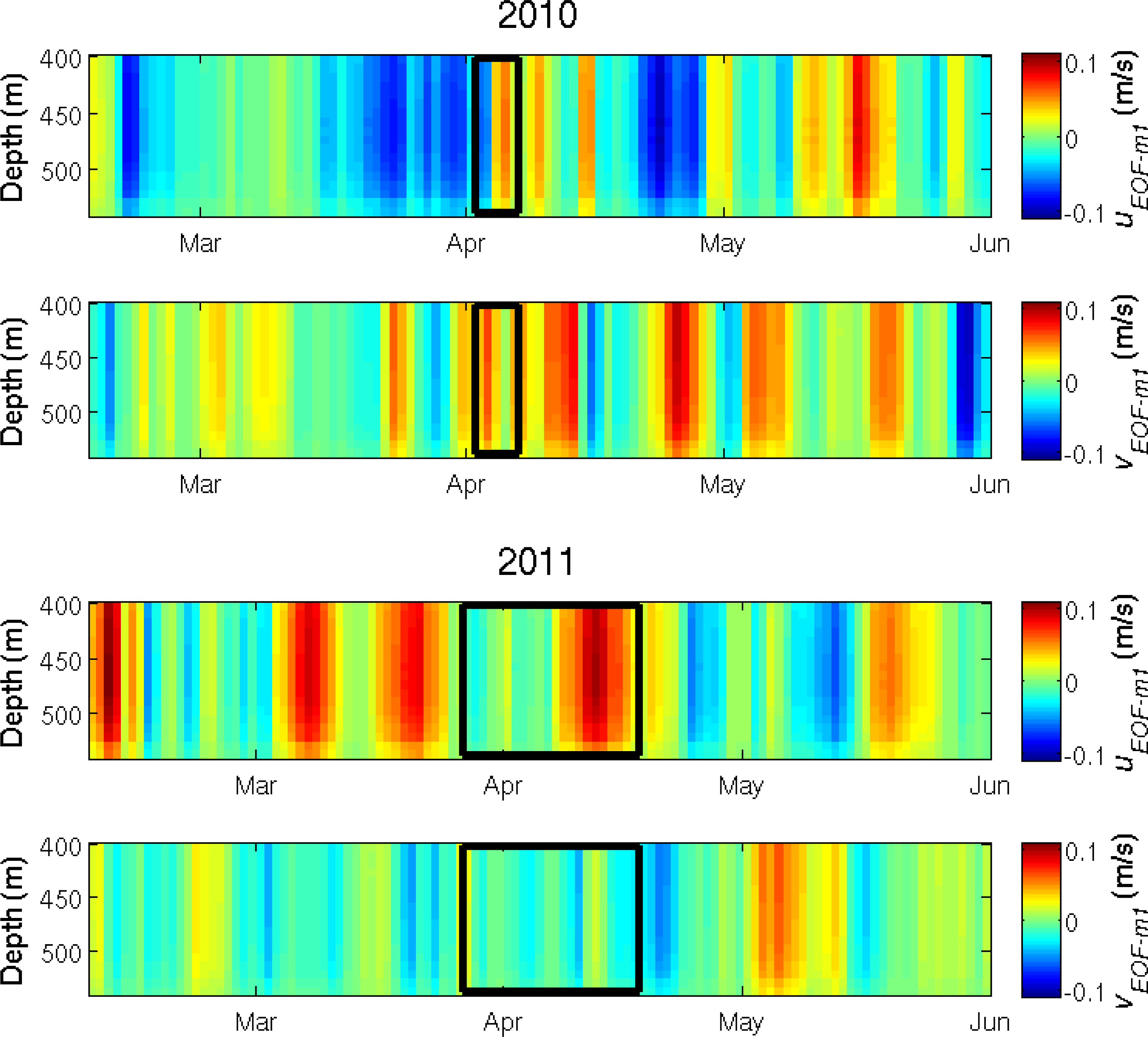
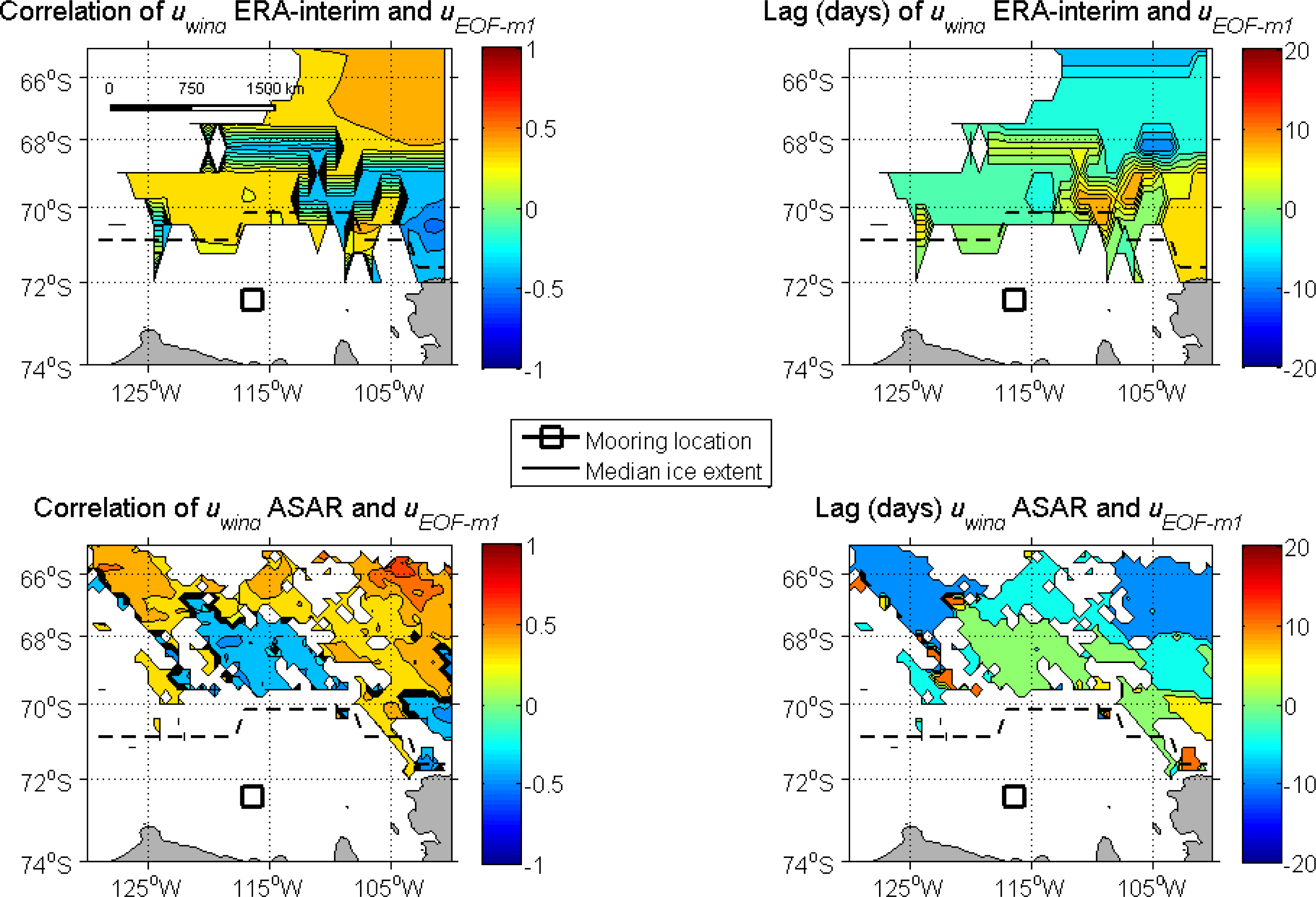
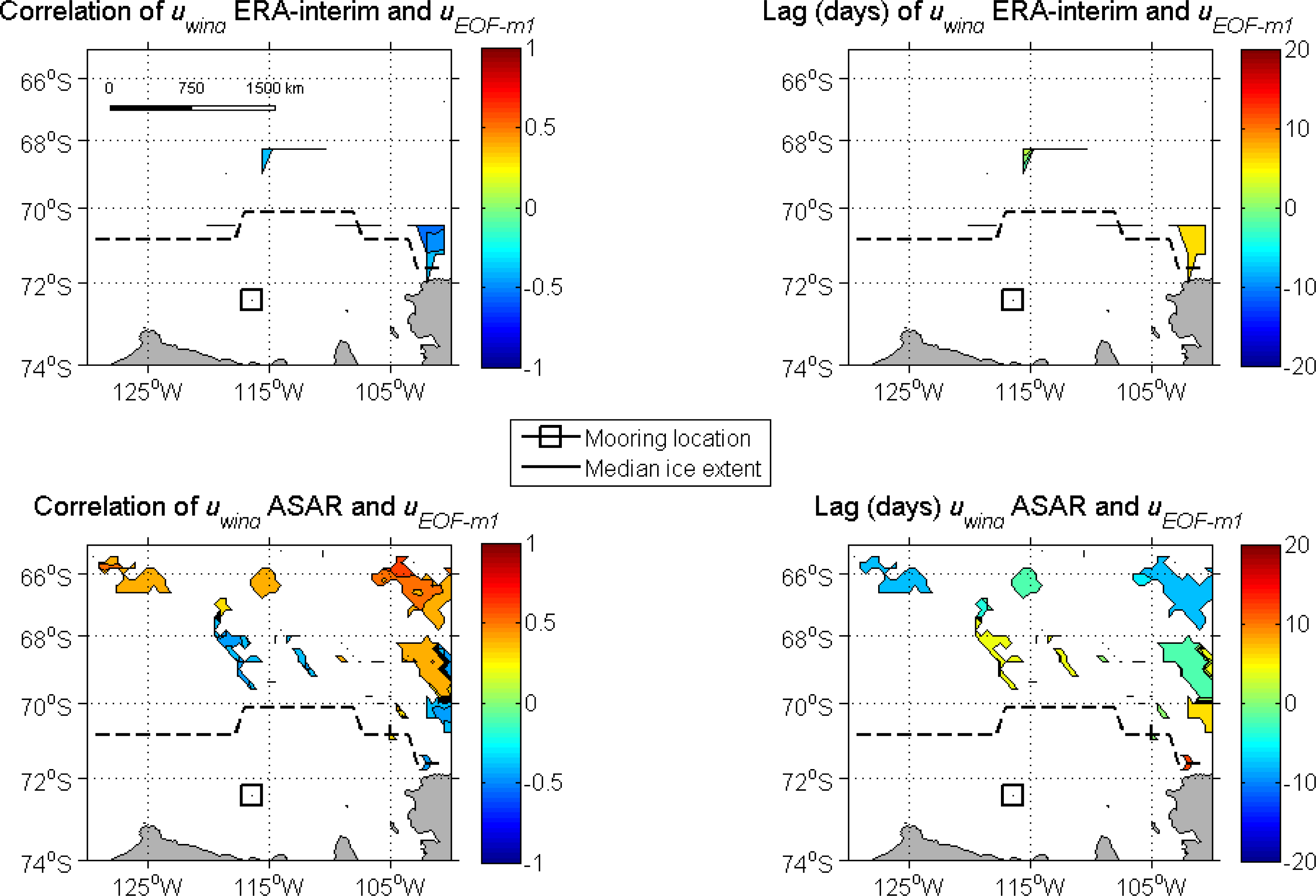
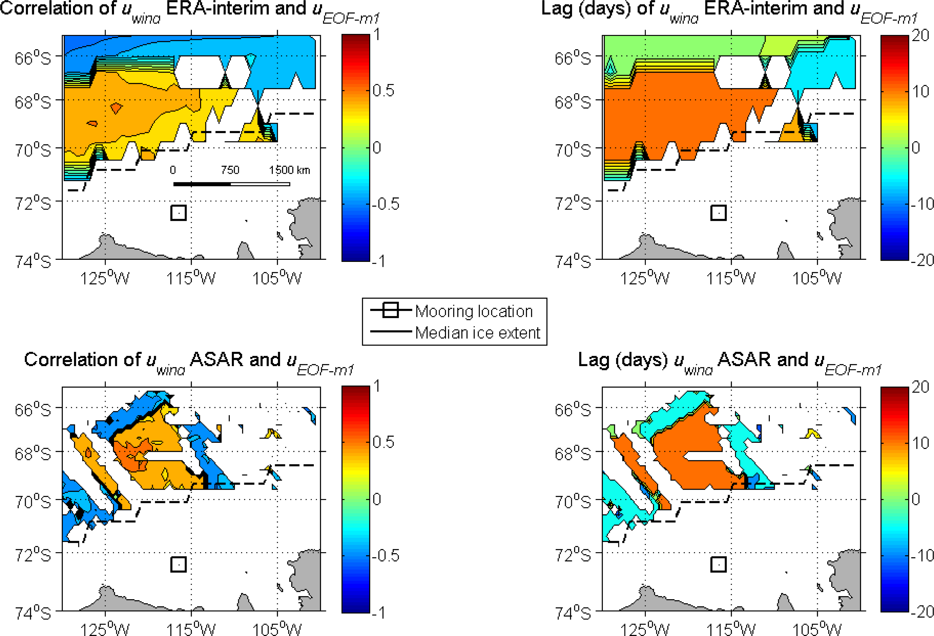
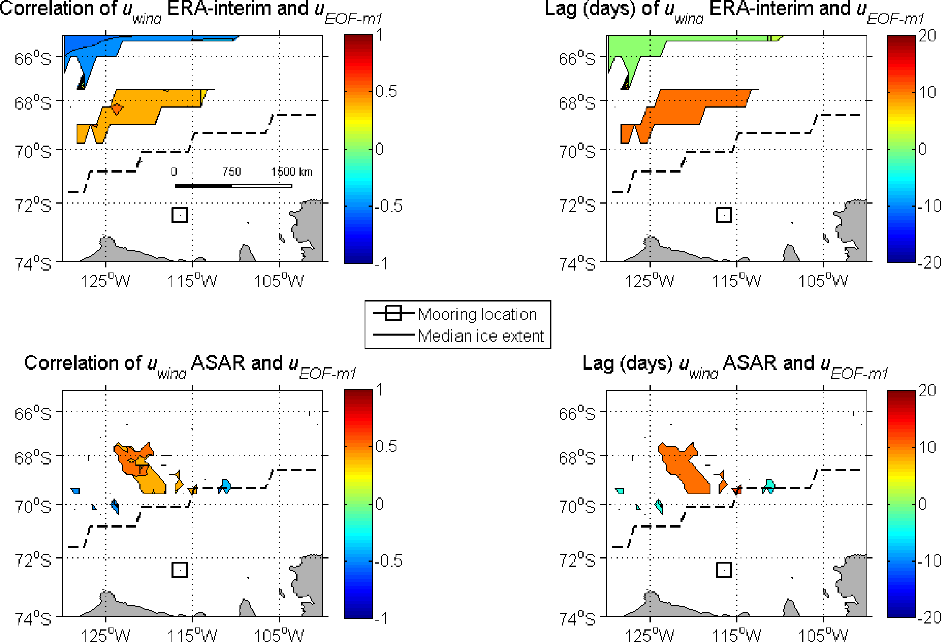
4.2. Correlations between Zonal Winds and Deep Water Velocities

The two example periods described in Section 4.1 indicate that the wind as measured by SAR images influences the deep currents observed by the mooring, in a way that is consistent with Ekman theory (Figure 1). For the second time period a possible delayed response was noted. This can be either an artifact of data gaps or a real effect, e.g., caused by strong persistent winds blowing over an ice sheet. In order to quantify the relationship between deep currents and the SAR derived wind, the statistical correlation between the wind and the deep current has been calculated for different time lags between the series. Figures 10 and 11 show maps for the maximum cross correlation between u_EOF–m1 and u_wind (Figure 10a), and time lag (Figure 10b) during 2010, for 95% and 99% confidence intervals, respectively. White areas indicate that the correlation was not statistically significant [13].

As mentioned in Section 3, the ice covered areas were masked out. Although the removal of the ice-covered areas reduces the number of data points in the southern part of the study area, the correlation is still significant in areas outside the ice covered parts. For 95% confidence interval (Figure 10) the correlation values as well as time lag for maximum correlation varies significantly, indicating that the confidence level may be too low. With 99% confidence interval (Figure 11), the areas with significant correlation are reduced. The coverage of significant correlations for u_wind from ASAR is larger than for the ERA-interim data. The results also indicate negative correlations for ERA-interim winds, while ASAR winds include also positive correlations, with a maximum of R = 0.71 at about 65.6°S and 104°W. This fact is probably due to the better resolution of the ASAR data.

Figure 12 shows the 2010 maps of maximum correlation between v_EOF–m1 and u_wind, and the lag for maximum correlation, for statistical significances of 95%, and an averaging period of two days. The results are similar for ERA interim and ASAR wind speeds and show a negative correlation with zero lag for an area around 70°S and 66°S and 105°W and 100°W. This was also noted in [13] and is probably caused by the presence of the Amundsen Low that gives predominantly southerly winds in this region when the winds over the outer shelf are westerly. For a 99% significance level (not shown here), the areas with correlations between v_EOF–m1 and u_wind were greatly reduced.

The relatively short average lag between u_wind and u_EOF–m1 in 2010 is consistent with study case 1 in 2010 (Figures 6 and 8), which indicated a rapid change of sign of u_EOF–m1 when the wind changed direction. However, the varying sign of the significant correlations and time lags indicates a complex relationship between u_wind and u_EOF–m1.

Figures 13 and 14 show the correlation between u_wind and u_EOF–m1 for 2011, analogous to Figures 10 and 11. The areas of significant correlation are larger and there is less variation in the time lags than in 2010. The effect of increasing the confidence level from 95% to 99% is mainly to reduce the area of significance. The area of positive significant correlation between u_wind and u_EOF–m1 located between 69.5°S and 67.5°S and 124°W and 115°W, with a lag of 10 days and a maximum correlation of 0.51 for ERA-interim winds and 0.62 for ASAR wind speed retrievals. The surface current below drifting sea ice is forced by the stress between sea ice and water, and not by the stress between wind and water. The drift of sea ice due to wind depends on the ice thickness and quality and internal deformation in the ice sheet [31]. If a uniform wind blows over an ice-covered region, the ice will after a certain time (depending on the thickness of the ice and its mass/inertia) move at an angle to the left of the wind direction (in the Southern Hemisphere). The resulting Ekman transport in the surface water is similar to the one in open water. However, since internal ice dynamics also affect the force balance then the momentum transfer from the wind via ice to the water can be very different from the transfer between wind and water, at least initially. The sea ice cover filters out small fluctuations in the wind but if the wind is uniform and persistent, an Ekman transport similar to the one in ice-free waters is expected although it could take some time to develop. It is hypothesized that the greater lag (10 days) observed for the maximum correlation in the year 2011 can be due to internal ice dynamics since there was more ice present in this year. However, the larger ice cover also means that there are fewer data points which also affect the statistical analysis. The correlations between u_wind and v_EOF–m1 were not statistically significant during 2011 Therefore, u_EOF–m1 represents the component describing most of the variability of the velocities detected in the mooring, expected to be affected by the Ekman pumping caused by the wind field, and having an influence on the melting of the ice sheet in the Amundsen Sea.

The maximum correlations found in the present study between the ASAR wind speeds and mooring data (0.71 for 2010 and 0.62 for 2011) are significantly larger than the maximum of 0.41 obtained with ERA-interim wind data in [13], based on the same mooring data. It is concluded that the selection of a time period with low ice coverage and the removal of ice covered areas from the analysis has significantly increased the correlation. The reason may be that the wind data (both in reanalysis products and in ASAR retrievals) is more accurate in ice-free waters, or that the Ekman circulation (Figure 1) is more directly coupled to the wind field in ice-free waters. The results do not appear to be sensitive to the choice of algorithm for inversion of wind speed, and similar correlation maps were obtained with CMOD-IFR2, CMOD5 as well as CMOD5.N GMFs.

The availability of ASAR WSM data is a limiting factor in the present study, and it is expected that the areas of significant correlation might increase with more available data. When the averaging was increased to three to five days, the areas of significant correlation were reduced.

It should also be taken into account that this study used ERA-interim wind directions, which have not been validated with data from the Amundsen Sea. The ERA-interim wind also has lower resolution than the wind speed retrievals from ASAR. Supposing correctness in the ERA-interim wind fields (commonly used as a reference for validation [32,33]), the mismatch between its resolution (0.75° in latitude and longitude) and the SAR wind cells present a source of error for wind directions with variations in scales smaller than the ERA-interim resolution. Nevertheless, although with low temporal resolution, the results achieved with the available ASAR data had a finer spatial delimitation and higher levels of significance than the corresponding results with ERA-interim wind speeds. The SAR wind retrievals are hence complementary to the ERA-interim and other reanalysis products, and provide a valuable addition for the investigation of the physics relating to surface wind interactions with the dynamics in the interior of the oceans.

A possible way to expand this study would be to increase the coverage of the study area further north. However, ASAR WSM imagery available for the Amundsen Sea (and generally for the Antarctica) was commonly restricted to a maximum latitude from −65°S to −64°S. This could be overcome with future data from the Sentinel-1 SAR sensor. It may also be relevant to include remotely sensed ice drift for areas covered by sea ice and combine with the wind maps to generate a merged data set with the ocean surface stress induced by wind or ice. Such a data set would cover the southern parts of the Amundsen Shelf that had only few data points in the present study.

5. Conclusions

This paper presents the temporal and spatial correlation between the wind field and the current velocity in one of the deep troughs leading from the shelf break to the glaciers in the Amundsen Sea. Wind data from both ERA-interim analysis and wind speed inversions from SAR images have been used. The SAR retrievals had higher spatial resolution but lower temporal resolution than the ERA-interim data, and the two methods are hence complementary. Both SAR and ERA interim data have larger uncertainties in the presence of sea ice, for which reason the study period was restricted to between 16 February and 31 May 2010 and 8 February to 31 May 2011. The high-resolution SAR wind maps were used to interpret two marked switches in ocean current direction (Figures 8 and 9). The results suggest that the wind field was the cause of the switches. The correlation between the current and the two wind data sources was quantified, and a statistically significant correlation between on-shelf currents and eastward wind was obtained for both data sets. The highest correlation, R = 0.71, was obtained for the SAR data. This correlation explains 71% of the variance of the current, and indicates that the wind is indeed the main forcing factor for the highly variable current along the deep trough in the central Amundsen Sea. It is suggested that the previously obtained, comparably low, correlation (R = 0.41, see [13]) is a combination of the poorer wind data quality and complex interaction between wind, sea ice and Ekman currents in ice covered waters. The SAR wind retrievals hence provided a valuable addition for the investigation of the physics relating surface wind interactions with the dynamics in the interior of the oceans. Significant advances for future studies of remotely sensed wind fields in this climatologically important part of the world could be made by developing techniques that are valid in sea ice, and obtaining longer time series of wind field as well as ocean currents.

References

1. Shepherd, A.; Wingham, D.J.; Mansley, J.A.D.; Corr, H.F.J. Inland thinning of Pine Island Glacier, West Antarctica. Science 2001, 291, 862–864. [Google Scholar]
2. Shepherd, A.; Wingham, D.; Rignot, E. Warm ocean is eroding West Antarctic Ice Sheet. Geophys. Res. Lett 2004, 31, 1–4. [Google Scholar]
3. Pritchard, H.D.; Arthern, R.J.; Vaughan, D.G.; Edwards, L.A. Extensive dynamic thinning on the margins of the Greenland and Antarctic ice sheets. Nature 2009, 461, 971–975. [Google Scholar]
4. Pritchard, H.D.; Ligtenberg, S.R.M.; Fricker, H.A.; Vaughan, D.G.; Van Den Broeke, M.R.; Padman, L. Antarctic ice-sheet loss driven by basal melting of ice shelves. Nature 2012, 484, 502–505. [Google Scholar]
5. Klinck, J.M.; Hofmann, E.E.; Beardsley, R.C.; Salihoglu, B.; Howard, S. Water-mass properties and circulation on the west Antarctic Peninsula Continental Shelf in Austral Fall and Winter 2001. Deep Sea Res. Part II: Top. Stud. Oceanogr 2004, 51, 1925–1946. [Google Scholar]
6. Moffat, C.; Owens, B.; Beardsley, R.C. On the characteristics of Circumpolar Deep Water intrusions to the west Antarctic Peninsula Continental Shelf. J. Geophys. Res. C: Oceans 2009, 114, C05017. [Google Scholar]
7. Dinniman, M.S.; Klinck, J.M.; Smith, W.O. A model study of Circumpolar Deep Water on the West Antarctic Peninsula and Ross Sea continental shelves. Deep Sea Res. Part II: Top. Stud. Oceanogr 2011, 58, 1508–1523. [Google Scholar]
8. Walker, D.P.; Brandon, M.A.; Jenkins, A.; Allen, J.T.; Dowdeswell, J.A.; Evans, J. Oceanic heat transport onto the Amundsen Sea shelf through a submarine glacial trough. Geophys. Res. Lett. 2007. [Google Scholar] [CrossRef] [Green Version]
9. Wåhlin, A.K.; Yuan, X.; Björk, G.; Nohr, C. Inflow of warm circumpolar deep water in the central Amundsen shelf. J. Phys. Oceanogr 2010, 40, 1427–1434. [Google Scholar]
10. Jacobs, S.; Jenkins, A.; Hellmer, H.; Giulivi, C.; Nitsche, F.; Huber, B.; Guerrero, R. The Amundsen Sea and the Antarctic ice sheet. Oceanography 2012, 25, 154–163. [Google Scholar]
11. Thoma, M.; Jenkins, A.; Holland, D.; Jacobs, S. Modelling circumpolar deep water intrusions on the Amundsen Sea continental shelf, Antarctica. Geophys. Res. Lett 2008, 35, L18602. [Google Scholar]
12. Steig, E.J.; Ding, Q.; Battisti, D.S.; Jenkins, A. Tropical forcing of circumpolar deep water inflow and outlet glacier thinning in the amundsen sea embayment, west antarctica. Ann. Glaciol 2012, 53, 19–28. [Google Scholar]
13. Wåhlin, A.K.; Kalén, O.; Arneborg, L.; Björk, G.; Carvajal, G.K.; Ha, H.K.; Kim, T.W.; Lee, S.H.; Lee, J.H.; Stranne, C. Variability of warm deep water inflow in a submarine trough on the Amundsen Sea shelf. J. Phys. Oceanogr. 2013. [Google Scholar] [CrossRef]
14. Pedlosky, J. Geophysical Fluid Dynamics, 2nd ed; Springer-Verlag: New York, NY, USA; p. 1987.
15. Christiansen, M.; Koch, W.; Horstmann, J.; Bay Hasager, C.; Nielsen, M. Wind resource assessment from C-band SAR. Remote Sens. Environ 2006, 105, 68–81. [Google Scholar]
16. Carvajal, G.K.; Eriksson, L.E.B.; Ulander, L.M.H. Retrieval and quality assessment of wind velocity vectors on the ocean with C-band SAR. IEEE Trans. Geosci. Remote Sens. 2013. [Google Scholar] [CrossRef]
17. Dee, D.P.; Uppala, S.M.; Simmons, A.J.; Berrisford, P.; Poli, P.; Kobayashi, S.; Andrae, U.; Balmaseda, M.A.; Balsamo, G.; Bauer, P.; et al. The ERA-interim reanalysis: Configuration and performance of the data assimilation system. Q. J. R. Meteorol. Soc 2011, 137, 553–597. [Google Scholar]
18. Arneborg, L.; Wahlin, A.K.; Björk, G.; Liljebladh, B.; Orsi, A.H. Persistent inflow of warm water onto the central Amundsen shelf. Nature Geosci 2012, 5, 876–880. [Google Scholar]
19. Pawlowicz, R.; Beardsley, B.; Lentz, S. Classical tidal harmonic analysis including error estimates in MATLAB using T_TIDE. Comput. Geosci 2002, 28, 929–937. [Google Scholar]
20. Davis, R.E. Predictability of sea level pressure anomalies over the North Pacific Ocean. J. Phys. Oceanogr 1978, 8, 233–246. [Google Scholar]
21. Quilfen, Y.; Chapron, B.; Elfouhaily, T.; Katsaros, K.; Tournadre, J. Observation of tropical cyclones by high-resolution scatterometry. J. Geophys. Res. C: Oceans 1998, 103, 7767–7786. [Google Scholar]
22. Hersbach, H.; Stoffelen, A.; De Haan, S. An improved C-band scatterometer ocean geophysical model function: CMOD5. J. Geophys. Res. C: Oceans 2007, 112, C03006. [Google Scholar]
23. Hersbach, H. Comparison of C-Band scatterometer CMOD5.N equivalent neutral winds with ECMWF. J. Atmos. Ocean. Technol 2010, 27, 721–736. [Google Scholar]
24. Furevik, B.R.; Johannessen, O.M.; Sandvik, A.D. SAR-retrieved wind in polar regions—Comparison with in situ data and atmospheric model output. IEEE Trans. Geosci. Remote Sens 2002, 40, 1720–1732. [Google Scholar]
25. Koch, W. Directional analysis of SAR images aiming at wind direction. IEEE Trans. Geosci. Remote Sens 2004, 42, 702–710. [Google Scholar]
26. Alpers, W.; Brummer, B. Atmospheric boundary layer rolls observed by the synthetic aperture radar aboard the ERS-1 satellite. J. Geophys. Res 1994, 99, 12613–12621. [Google Scholar]
27. Hansen, M.W.; Collard, F.; Dagestad, K.F.; Johannessen, J.A.; Fabry, P.; Chapron, B. Retrieval of sea surface range velocities from envisat ASAR doppler centroid measurements. IEEE Trans. Geosci. Remote Sens 2011, 49, 3582–3592. [Google Scholar]
28. Alexander, M.A.; Bhatt, U.S.; Walsh, J.E.; Timlin, M.S.; Miller, J.S.; Scott, J.D. The atmospheric response to realistic Arctic sea ice anomalies in an AGCM during winter. J. Clim 2004, 17, 890–905. [Google Scholar]
29. National Snow and Ice Data Center: Advancing knowledge of Earth’s frozen regions. Available online: http://nsidc.org/cryosphere/seaice/data/terminology.html (accessed on 21 March 2013).
30. Sciremammano, F. A suggestion for the presentation of correlations and their significance levels. J. Phys. Oceanogr 1979, 9, 1273–1276. [Google Scholar]
31. Worby, A.P.; Bindoff, N.L.; Lytle, V.I.; Allison, I.; Massom, R.A. Winter ocean/sea ice interactions studied in the east Antarctic. Eos Trans. AGU 1996, 77, 453–457. [Google Scholar]
32. Verspeek, J.; Stoffelen, A.; Portabella, M.; Bonekamp, H.; Anderson, C.; Saldaña, J.F. Validation and calibration of ASCAT using CMOD5.N. IEEE Trans. Geosci. Remote Sens 2010, 48, 386–395. [Google Scholar]
33. Montuori, A.; De Ruggiero, P.; Migliaccio, M.; Pierini, S.; Spezie, G. X-band COSMO-SkyMed wind field retrieval, with application to coastal circulation modeling. Ocean Sci 2013, 9, 121–132. [Google Scholar]
Figure 1. Sketch of the wind-driven Ekman transport (blue) in the Southern Hemisphere, together with the return flow (red) which the mooring (sketched on the bottom) measures.
Remotesensing 05 04088f1
Figure 2. Map of the region, with the position of the mooring indicated by a blue triangle. Grey areas below the coast line indicate grounded ice sheet, purple areas indicate ice shelves (the floating part of the ice sheet). Red arrows indicate the topographic steering by the bathymetric trough: Ocean currents have a strong tendency to flow along isobaths, and hence water that moves across the shelf tends to concentrate to troughs or ridges leading from the shelf break to the inner shelf.
Remotesensing 05 04088f2
Figure 3. Daily values of ERA-interim analysis averaged over the area 74°S to 65°S and 130°W to 100°W.
Remotesensing 05 04088f3
Figure 4. ERA-interim reanalysis data averaged over January to May 2010 (a) and January to May 2011 (b). Top panels show zonal wind component, middle panels show meridional wind component, lower panels show ice concentration (in percentage of time that the area was ice covered). The location of the mooring is indicated by the white rectangle.
Remotesensing 05 04088f4
Figure 5. Daily average of the first Empirical Orthogonal Function (EOF) mode of the detided along-trough (uEOF–m1) and across trough (vEOF–m1) velocities detected by the S1 mooring at 72.45°S and 116.34°W. Black rectangles indicate time periods selected to investigate the relationship with wind data.
Remotesensing 05 04088f5
Figure 6. Hourly average of the first Empirical Orthogonal Function (EOF) mode of the detided along-trough (uEOF–m1) and across trough (vEOF–m1) velocities measured by the S1 mooring at 72.45°S and 116.34°W for the study cases highlighted in Figure 5.
Remotesensing 05 04088f6
Figure 7. Examples of georeferenced Envisat advanced synthetic aperture radar wide swath mode (ASAR WSM) images used for the computation of wind maps in the Amundsen Sea. The location of the mooring is indicated by the black rectangle.
Remotesensing 05 04088f7
Figure 8. ASAR wind maps for study case 1 on 3 and 6 April 2010. ASAR wind speeds are indicated by the color and the small black arrows indicate the wind direction from the ERA-interim data. Dashed black arrows illustrate directions associated with the Ekman transport and red arrows the current observed at the mooring (black rectangle frame).
Remotesensing 05 04088f8
Figure 9. ASAR wind maps for study case 2 between 27 March and 17 April 2011. ASAR wind speeds are indicated by the color and the black arrows indicate the wind direction from the ERA-interim data.
Remotesensing 05 04088f9aRemotesensing 05 04088f9b
Figure 10. Correlation (a) and lag (b) with 95% confidence interval between zonal wind and uEOF–m1 during 2010. The time series of the wind component in each grid point has been averaged in two-day intervals and has been computed for ASAR wind speed retrievals from 16 February until 31 May 2010.
Remotesensing 05 04088f10
Figure 11. As Figure 10 for 99% of statistical significance.
Remotesensing 05 04088f11
Figure 12. As Figure 10 for vEOF–m1.
Remotesensing 05 04088f12
Figure 13. Correlation and lag with 95% of statistical significance between zonal wind and uEOF–m1 during 2011. The time series of the wind component in each grid point has been averaged in two-day intervals and has been computed for ASAR wind speed retrievals from the 8 February until the 31 May 2011. The time lag is expected to vary depending on the shape of the wind field.
Remotesensing 05 04088f13
Figure 14. As Figure 13 for 99% of statistical significance.
Remotesensing 05 04088f14