Characterizing the Absorption Properties for Remote Sensing of Three Small Optically-Diverse South African Reservoirs


Abstract
: Characterizing the specific inherent optical properties (SIOPs) of water constituents is fundamental to remote sensing applications. Therefore, this paper presents the absorption properties of phytoplankton, gelbstoff and tripton for three small, optically-diverse South African inland waters. The three reservoirs, Hartbeespoort, Loskop and Theewaterskloof, are challenging for remote sensing, due to differences in phytoplankton assemblage and the considerable range of constituent concentrations. Relationships between the absorption properties and biogeophysical parameters, chlorophyll-a (chl-a), TChl (chl-a plus phaeopigments), seston, minerals and tripton, are established. The value determined for the mass-specific tripton absorption coefficient at 442 nm, (442), ranges from 0.024 to 0.263 m2·g−1. The value of the TChl-specific phytoplankton absorption coefficient ( ) was strongly influenced by phytoplankton species, size, accessory pigmentation and biomass. (440) ranged from 0.056 to 0.018 m2·mg−1 in oligotrophic to hypertrophic waters. The positive relationship between cell size and trophic state observed in open ocean waters was violated by significant small cyanobacterial populations. The phycocyanin-specific phytoplankton absorption at 620 nm, (620), was determined as 0.007 m2·g−1 in a M. aeruginosa bloom. Chl-a was a better indicator of phytoplankton biomass than phycocyanin (PC) in surface scums, due to reduced accessory pigment production. Absorption budgets demonstrate that monospecific blooms of M. aeruginosa and C. hirundinella may be treated as “cultures”, removing some complexities for remote sensing applications. These results contribute toward a better understanding of IOPs and remote sensing applications in hypertrophic inland waters. However, the majority of the water is optically complex, requiring the usage of all the SIOPs derived here for remote sensing applications. The SIOPs may be used for developing remote sensing algorithms for the detection of biogeophysical parameters, including chl-a, suspended matter, tripton and gelbstoff, and in advanced remote sensing studies for phytoplankton type detection.1. Introduction
Knowledge of the inherent optical properties (IOPs), including the absorption of phytoplankton, gelbstoff (or chromophoric dissolved organic matter) and tripton (non-living minerals and detritus), is critical to water remote sensing. IOPs are required for remote sensing algorithm development and for physically-based bio-optical models simulating the behavior of light in water (e.g., [1]). Physically-based water constituent retrieval remote sensing algorithms, especially those targeting specific water types or classes, rely heavily on IOPs, as do biogeochemical models. As a result, much attention has been given to determining the variability in the absorption properties of coastal and open-ocean marine waters (e.g., [2–4]). Recent studies have also sought to characterize the absorption properties of optically-complex inland and estuarine waters (e.g., [5–10]). However, there is an ongoing need to investigate the variability that might be encountered across these diverse systems, especially those that are hypertrophic. This poses an ongoing challenge for satellite-based remote sensing applications aimed at characterizing the phenology and ecological state of Earth’s precious and vulnerable fresh waters.
In water-scarce South Africa, man-made reservoirs provide an essential source of potable water to a growing urban population. Widespread eutrophication and cyanobacterial blooms have degraded water quality in many of these reservoirs, posing a potential health threat to millions of consumers, as well as for industrial and commercial users [11]. Data on the optical characteristics and variability of these reservoirs is lacking, hindering present and future monitoring efforts using remote sensing. This paper aims to describe the variability in the absorption properties of phytoplankton, gelbstoff and tripton of three optically-diverse South African reservoirs. It describes the relationships between absorption and biogeophysical variables, chlorophyll-a (chl-a), seston (total suspended solids) and mineral dry weight. The chl-a-specific absorption coefficients ( ) are determined for the diverse phytoplankton assemblages and discussed with reference to typical values reported in Case 1 waters. The variability of the phycocyanin (PC)-specific absorption at 620 nm, (620), used in semi-analytical algorithms aimed at the detection of PC (e.g., [12,13]), is also determined for cyanobacterial blooms and in surface scums of Microcystis aeruginosa. The mass-specific tripton absorption coefficients ( ) are determined using a modified technique and the results compared to reported values from inland and coastal waters. Finally, absorption budgets are presented for each of the reservoirs. The aims of the paper are to provide a thorough description of the range of variability in absorption properties that might typically be encountered in South African inland waters, and to provide IOPs for use in remote sensing radiative transfer studies and physically-based water constituent retrieval algorithms (see Matthews and Bernard [14]).
2. Methods
2.1. Study Areas and Sampling Strategy
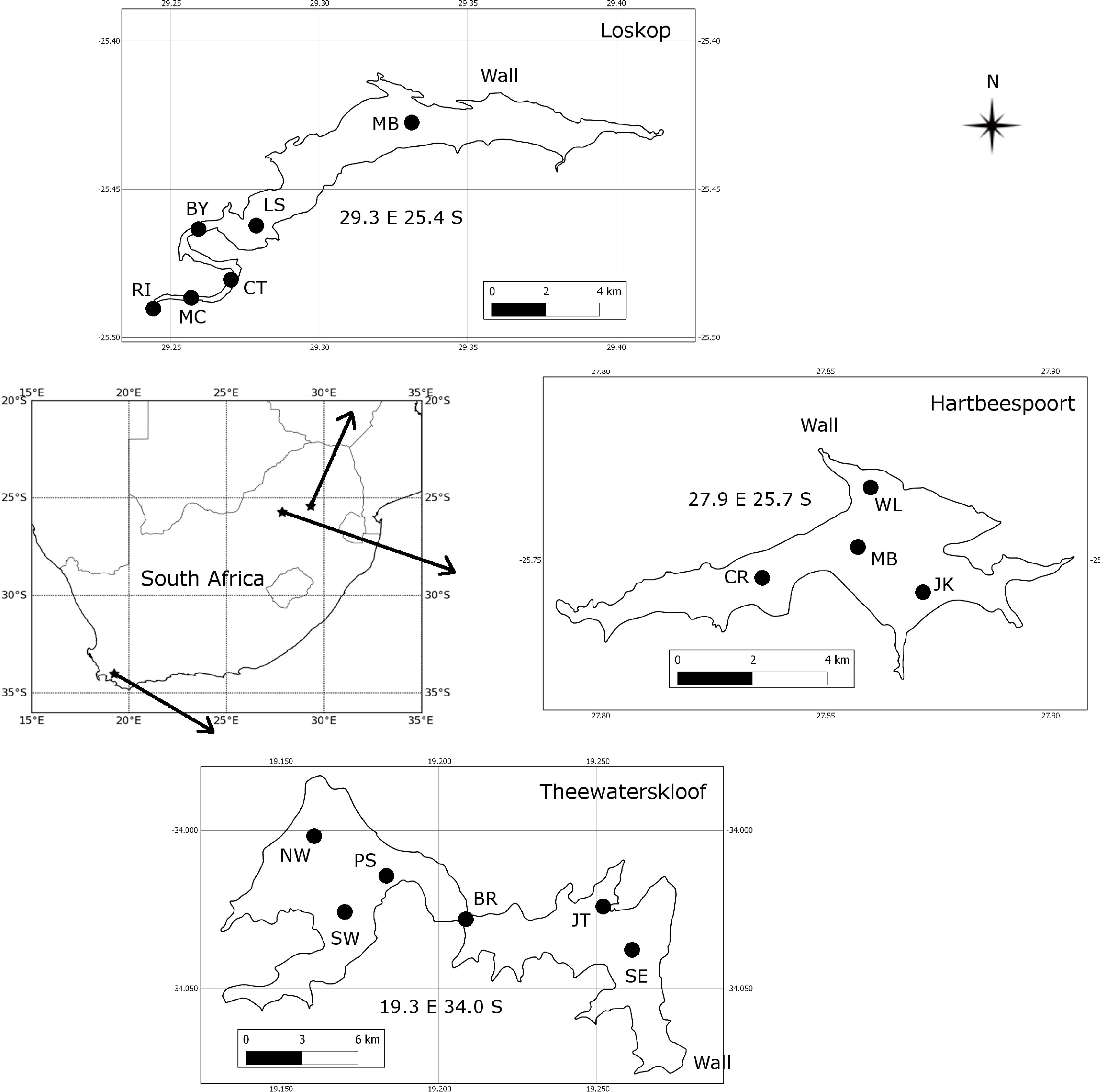
The three study areas, Hartbeespoort, Loskop and Theewaterskloof reservoirs, were chosen in order to capture some of the diverse range of water types and blooms occurring in South African inland waters (Figure 1). Sampling campaigns were undertaken at each of the lakes for a three week period: at Hartbeespoort in October 2010, at Loskop in July/August 2011, and at Theewaterskloof in April 2012. Sample points (see Figure 1) were located so as to capture the diversity of water conditions occurring in each of the reservoirs. Surface water samples were collected in 1 L plastic containers or in 5 L opaque plastic buckets following thorough rinsing with lake water. Every effort was made to avoid disturbing the dense aggregations of cyanobacteria on the water surface (when present) by gently collecting water into containers held horizontally. Samples were kept in the dark and on ice until analysis. Water clarity was measured using a Secchi disk, zsd, using the mean of the depth at which the disk disappeared and then re-appeared.
Of the three study areas, Hartbeespoort is the most extensively studied, followed by Loskop, while Theewaterskloof is almost undescribed in the scientific literature. Detailed information on the limnology and phytoplankton dynamics of Hartbeespoort is available (e.g., [15–17]). It is one of the most productive reservoirs in the world, with so-called hyperscums of Microcystis Aeruginosa [18]. Measurements of its optical properties, however, are limited to light attenuation [19,20]. The water quality and phytoplankton assemblage of Loskop has previously been described [21–23]. Situated on the Olifants River, Loskop has very diverse water types, due to its longitudinal zonation, with pronounced riverine, transitional and lacustrine zones [22]. The water is affected by acid mine drainage and has high concentrations of heavy metals and nutrients (ibid.). However, no detailed limnological study of the reservoir has been undertaken, and information on its light environment is limited to a Secchi disk. Theewaterskloof is located in the western winter rainfall region of South Africa and is one of the primary water supply reservoirs for the Cape Town region through an inter-basin transfer scheme. The reservoir is divided into two basins by a narrow channel crossed by a bridge; the western basin contains the inlet from the Sonderend River and the eastern basin, the dam wall. Despite its great importance as a potable water supply, there is no published information on its limnology, phytoplankton assemblage or light environment.
2.2. Phytoplankton Pigments
Water samples were filtered under low pressure (>10 mm mercury pressure) through Whatmann GF/F filters on the same day as collection. The concentrations of chl-a and phaeopigments were determined spectrophotometrically using an extraction solution of 90% boiling ethanol after Sartory and Grobbelaar [24], due to the improved extraction efficiency of ethanol with freshwater phytoplankton assemblages containing cyanobacteria. TChl is defined as the sum of chl-a and phaeopigments. Phycocyanin (PC) and allo-phycocyanin (APC) pigments were measured when cyanobacteria made up a significant portion of the phytoplankton assemblage. Cyanobacteria have very resistant cell walls that must be broken to release the water soluble phycobiliproteins. Various methods may be used to break the cell walls, including freezing and thawing [25], enzymatic attack [26], osmotic shock [27], attack by N fixing bacteria [28], acid, nitrogen cavitation and french press (see [28,29] for details). However, the most efficient methods appear to be freeze-thaw and enzymatic attack [28]. Therefore, a combination of these techniques was used after Beutler [30] to optimize extraction efficiency and to reduce the amount of time required for analysis in the field. Filter papers were frozen for at least 24 h in 15 mL screw capped tubes. If samples were being transported, they were stored in liquid nitrogen and, then, at −70 °C. After thawing, an extraction solution of 0.25 M Trizma Base, 10 mM disodium EDTA (Ethylenediaminetetraacetic acid) and 2 mg·mL−1 lysozyme was added. After grinding with a glass rod, the filter paper was incubated in the dark for 2 h at 37 °C and, then, stored in the cold for at least 20 h to allow for extraction. The samples were then diluted with Milli-Q water and centrifuged at 3,600 g for 15 min. to reduce turbidity. The supernatant was initially filtered through a 0.2 μm pore size membrane filter; however, this may interfere with the phycobiliproteins so subsequent analyses did not filter the supernatant [69]. The sample was read in the spectrophotometer using 1 cm matched quartz cuvettes using the extraction solution as the reference, and the PC concentration was calculated according to Bennett and Bogorad [31]. All pigment analyses were done in triplicate using the mean as the final value.
2.3. Seston, Minerals and Tripton Concentrations
Seston dry mass was determined using pre-ashed Whatmann GF/F filter papers following the gravimetric technique [32]. The inorganic component (here, referred to as minerals) was determined by burning the filter pads in a muffle furnace at 500 °C and re-weighing. All analyses were done in triplicate using the mean as the final value.
Tripton corresponds to the de-pigmented matter measured by the quantitative filter technique (QFT, see below). However, it is difficult to separate out the living phytoplankton component of seston in order to measure tripton dry mass. Determination of is useful for bio-optical models, because it allows for the particulate detrital and mineral components to be handled simultaneously and separately from living phytoplankton. Seston dry mass might be partitioned most simply into its tripton and phytoplankton components according to: tripton = seston − β × chla, where β is a conversion factor to estimate phytoplankton dry mass from chl-a. Most studies using this technique assume a constant value of β, most often equal to 0.07 g·mg−1 (e.g., [33–35]). However, the value of β varies widely in nature, according to the intracellular chl-a concentration, which is dependent on the species and the light and nutrient environment. For cyanobacteria P. hollandica and O. limnetica cultured under a range of light and nutrient conditions, Gons et al. [36] determined the value of β to range between 0.02–0.3 g·mg−1, mean = 0.046 g·mg−1. Zhang et al. [37] determined a value of 0.09 g·mg−1 for an assemblage dominated by Microcystis and Scenedesmus in lake Taihu, China. Desortová [38] determined that the chl-a content per unit fresh phytoplankton biomass for various lakes was between 0.14% and 3.41%, which corresponds to a β of 0.029–0.71 g·mg−1. The range of variability was primarily related to seasonal variation in solar radiation, with larger values being attributed to low-light conditions (winter months). Natural populations of individual cells of various species have mean values ranging from 0.0496 to 0.21 g·mg−1 (calculated from Table 1.3 in [39]).
In this study, values of β were determined by investigating the ratio of phytoplankton to detritus, Rpd. In steady-state conditions (i.e., loss rate = growth rate), Rpd should be constant, irrespective of the trophic state, with a value near 0.3 [36]. This is in agreement with reported values of Rpd in lakes, which are typically between 20% and 35% (e.g., [40,41]). In non-steady-state conditions, Rpd may vary; however, its value is expected to be less than one for almost all growth conditions [36]. The existence or non-existence of steady-state conditions was determined by examining the variability of the chl-a:seston ratio in time [36]. For conditions deemed to be in steady-state, values for β were selected where the corresponding Rpd values were near 0.3. On average, phytoplankton contains 10% mineral content (ash dry mass) [39]. Therefore, detrital dry weight was calculated according to: detritus = seston −0.9 × minerals − β × chla. Rpd was calculated using the detrital and phytoplankton dry mass calculated for a range of β values. Since ash dry weight was not determined in Hartbeespoort, minerals were assumed to be zero, which, in this case, might be a reasonable assumption (see results).
2.4. Absorption Coefficients of Particulate, Pigmented and Dissolved Substances
The QFT was used to determine the absorption of total particulate matter (seston) and de-pigmented matter (tripton) after Mitchell et al. [42]. Water samples were stored in the dark and analyzed on the same day as collection. The sample was filtered under low vacuum pressure (>10 mm mercury pressure) through a pre-ashed Whatman GF/F filter paper pre-washed with Milli-Q water, adjusting the volume according to the turbidity of the sample. In cases of very high biomass, such as Hartbeespoort (chl-a > 10,000 mg·m−3), as little as 2.5 mL was filtered, while for chl-a < 1 mg·m−3 in Loskop, up to 1 L was filtered to obtain sufficient material on the filter. Blank filter papers were treated identically to the sample, by simultaneously filtering the same volume of Milli-Q water as the sample. Care was taken to not run the blank filters dry. Filter papers were kept in labeled Petri dishes with a drop of water until analysis to ensure hydration.
The optical density (OD) of the particulate and blank filter paper between 350 and 850 nm was measured using a Shimadzu UV-2501 spectrophotometer using an ISR-2200 integrating sphere. The mean OD of the filter relative to the blank was near 0.5 for all samples. In the case of Hartbeespoort, however, the value was unavoidably higher, owing to the extremely high biomass. The mean OD of the blank measurements was subtracted from the particulate OD measurements and the absorption calculated using a pathlength amplification factor β = 2 [43]. A null subtraction was performed at the highest wavelength of measurement (=850 nm) as the assumption of no absorption from particulate matter at 750 nm does not hold in highly turbid inland waters. Duplicate particulate absorption measurements were performed for each sample, using the mean of the two spectra as the final value.
atr was determined by two methods, sodium hypochloride (NaClO) oxidation and, in the case of Theewaterskloof, boiling methanol extraction. Both of these techniques have been used for freshwater samples (e.g., [9,44]), but little information exists on what quantitative errors each of these methods might introduce. Since both methods remove non-chlorophyllous pigments (carotenoids and phaeopigments), the phytoplankton absorption will tend to be overestimated. The NaClO technique has two advantages in that it bleaches the water soluble phycobilipigments and resistant cells (e.g., chlorophytes), and it may be performed more rapidly in the field [45]. However, there is some evidence to suggest that NaClO treatment of samples with high dissolved organic matter may cause bleaching of colloidal/particle-bound organic matter, leading to overestimates of phytoplankton absorption in the blue spectrum [9]. Furthermore, NaClO is unsuitable for waters with a high abundance of heterotrophic bacteria, due to the production of a yellow cytochrome byproduct deposited on the filter [46]. Techniques using organic solvents methanol or ethanol (e.g., [12]) might avoid these effects, although it is uncertain to what degree phycobilipigments are removed, even when related absorption peaks are not visible in the absorption spectrum. Measurements were performed using both techniques in order to quantify and elucidate these errors. Complete pigment bleaching/extraction was assessed by the absence of the 675 nm chl-a absorption peak. In cases of insufficient bleaching/extraction, the filter paper was gently subjected to further bleaching/extraction until the 675 nm peak disappeared. The filters were thoroughly rinsed with Milli-Q water to remove contamination by NaClO in order to perform readings <400 nm. Blank filter papers were treated identically to samples. The mean bleached blank OD was subtracted from the bleached particulate OD to calculate the tripton absorption. The tripton absorption curves were fitted to an exponential function [47], and the slope coefficient, Str, was computed using a reference wavelength of 442 nm.
The phytoplankton absorption component was then computed as aϕ = ap − atr. The specific absorption coefficients, and , were determined by dividing aϕ and atr by the concentration of TChl and tripton, respectively. In order to calculate the PC-specific absorption coefficient, (620), a correction needs to be applied to aϕ(620) in order to remove the effect of residual chl-a absorption, termed achl(620). Simis et al. [12] determined the value of achl(620) from aϕ(665) using a ratio term, ε = 0.24. The absorption exclusively due to PC is then calculated by apc(620) = aϕ(620) − ∈ × aϕ(665). (620) is then calculated by apc(620)/PC. The value of ε determined by Simis et al. [12] is generally suitable for use in cyanobacteria-dominated waters and, therefore, is used here. No attempt was made to correct for algae containing other pigments influencing absorption near 665 and 620 nm (e.g., [48]). The absorbance due to gelbstoff, ag, was read between 340 and 750 nm in the spectrophotometer using matched 10 cm quartz cuvettes using room temperature Milli-Q water as the reference. A null-point correction at 750 nm was implemented and the absorption calculated according to Mitchell et al. [42]. The curves were fitted to an exponential function [47] between 350 and 500 nm, and the slope coefficient, Sg, was computed using a reference wavelength of 442 nm.
3. Results and Discussion
3.1. General Characteristics of Reservoirs
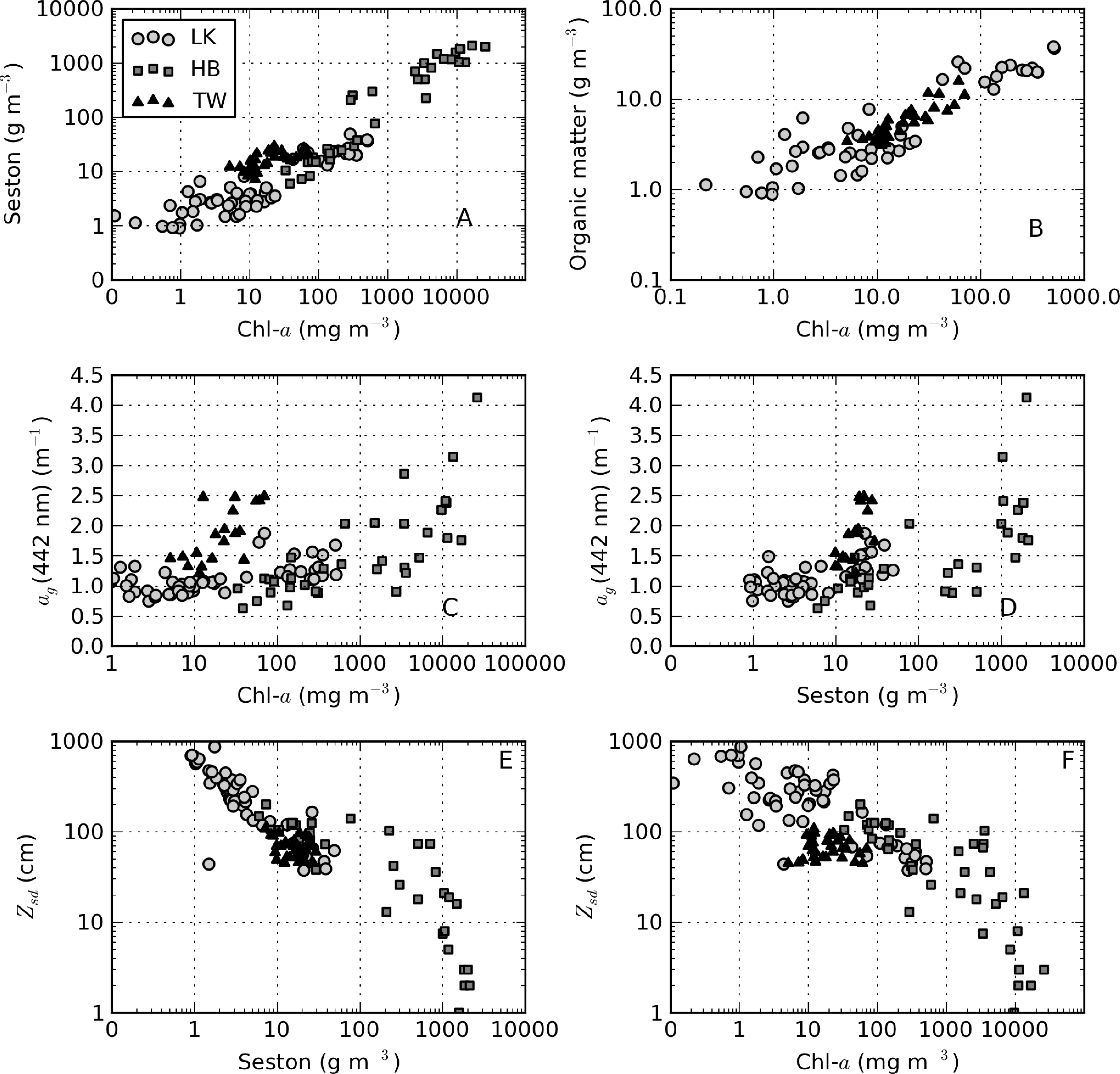
There was extremely large variability in biogeochemical and optical parameters between and within the three systems studied (Table 1). Figure 2 shows scatter plots of some parameters illustrating this variability, and the correlation coefficients for the entire dataset are shown in Table 2. Chl-a and seston are highly correlated (r = 0.92), with concentrations varying over six and five orders of magnitude, respectively (Figure 2A). The extremely high chl-a values >1,000 mg·m−3 were measured in surface scum conditions in Hartbeespoort. The greatest trophic range is found in Loskop, with chl-a varying from 0.5 to 500 mg·m−3, while Theewaterskloof has the least range. The organic component of seston, calculated as the difference between seston and minerals, is highly correlated with chl-a (r = 0.85, Figure 2B). Weak correlations between gelbstoff absorption at 442 nm, ag(442), and chl-a and seston are apparent (r = 0.63 and 0.54, respectively, Figure 2C,D). However, the considerable scatter implies that the relationship is reservoir-specific and that ag is largely controlled by catchment-related factors, rather than phytoplankton biomass or seston [49]. Water clarity (zsd) is inversely correlated to seston (r = −0.43) and its mineral and organic components and phytoplankton pigments (chl-a, r = −0.27, Figure 2E,F). These relationships might be applied between reservoirs, given the general inverse trend.
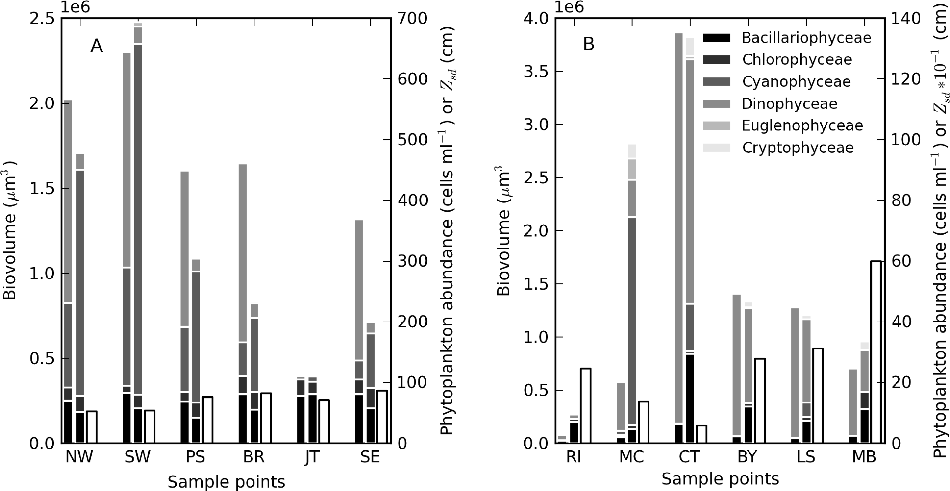
During the sampling period, M. aeruginosa composed more than 90% of the phytoplankton assemblage in Hartbeespoort (see Table 3). Bright green surface accumulations (10–50 cm thick) were present over most of the lake surface area. The concentration of chl-a and phycocyanin pigments were extremely high (up to 26,000 and 43,000 mg·m−3, respectively). In Loskop, the dinoflagellate, Ceratium hirundinella, is dominant throughout the reservoir in terms of biovolume, although cyanobacteria (in isolated blooms) and other species may be abundant (Figure 3B, Table 3). Working upstream, the main basin (point MB) is typically oligotrophic (chl-a < 1) and very clear, with a mixed population of diatoms, chlorophytes and dinoflagellates. The lacustrine zone (point LS) is oligotrophic (chl-a < 10), with slightly decreased water clarity. The transitional zone where a bio-optical buoy was moored (point BY) is more variable, due to mixing (1 < chl-a < 30). A dense bloom of the large-celled dinoflagellate C. hirundinella was present at point CT (Ceratium), turning the water dark brown, with chl-a values in excess of 200 mg·m−3. C. hirundinella blooms are common in South African reservoirs, causing a nuisance for water treatment [50,51]. A dense bright green surface bloom of M. aeruginosa was present further upstream at point MC (Microcystis). In summer, as water temperatures rise, the cyanobacteria become more abundant, and blooms extend downstream towards the transitional zone [22]. It appears that M. aeruginosa and C. hirundinella are competing species in the riverine zone. The inlet of the Olifants River at point RI (river input) is clear, with chlorophytes and diatoms being present. Loskop is, therefore, extremely diverse from both a trophic and color perspective.
Theewaterskloof is more uniform and turbid, with a mixed phytoplankton assemblage (Table 3) and a high mineralic component of dry weight (Table 1). The reservoir is affected by strong prevailing SE and NW winds (gusts up to 7.5 m·s−1 were measured), which means it is generally well-mixed. Blooms of filamentous cyanobacteria Anabaena ucrainica and a high abundance of diatom species, in particular, Aulacoseira ambigua and Asterionella formosa, are characteristic for the lake. The high mineralic component of dry weight might be related to the presence of these diatom species, which contain >40% ash weight of dry weight [39].
A general pattern of increasing turbidity and phytoplankton biomass can be observed from the eastern basin towards the western basin, near the inflow of the Sonderend River (Figure 3A). The eastern basin is mesotrophic (chl-a ≈ 10 mg·m−3). At the bridge (point BR), the water is typically meso-eutrophic with mixed blooms of cyanobacteria, chlorophytes and diatoms. The western basin (points SW and NW) is hyper/eutrophic with decreased water clarity (meanzsd = 50 cm) associated with the presence of a mixed bloom of Anabaena ucrainica and Sphaerodinium fimbriatum (Figure 3A). These species are co-dominant in terms of biovolume. During strong wind, sampling was carried out at point PS (pump station) near the water abstraction pump station.
3.2. Absorption by Gelbstoff
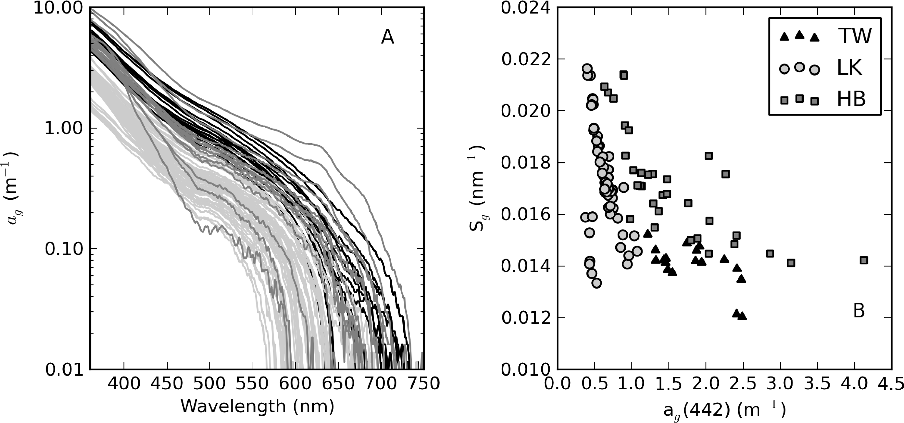
From an optical perspective, phytoplankton biomass and suspended particles appear to have greater influence on water clarity than dissolved organic matter, based on the observed water color. The measured ag curves are relatively consistent with an exponential function (straight lines in Figure 4A). ag(442) varies in a relatively narrow range from 0.63 to 4.13 m−1 (Table 1). Despite its large trophic gradient, Loskop has the most narrow range, from 0.75 to 1.87 m−1. Therefore, ag is essentially independent of trophic status. The widest range of values is found in Hartbeespoort (0.63 to 4.13 m−1), likely associated with extremely variable cyanobacterial biomass. Theewaterskloof has the highest average value of 1.9 m−1, which is consistent with the geological and floral environment associated with brackish Cape waters. An inverse relationship is generally present between Sg and ag(442); however, greater variability is associated with smaller values of ag(442) (see [3] Figure 4B). Sg ranges between 0.012 and 0.022 nm−1, within the range reported in coastal [3] and inland waters [49]. Mean values determined for Loskop and Hartbeespoort are 0.017 nm−1, while that for Theewaterskloof is 0.014 nm−1.
3.3. Absorption by Seston
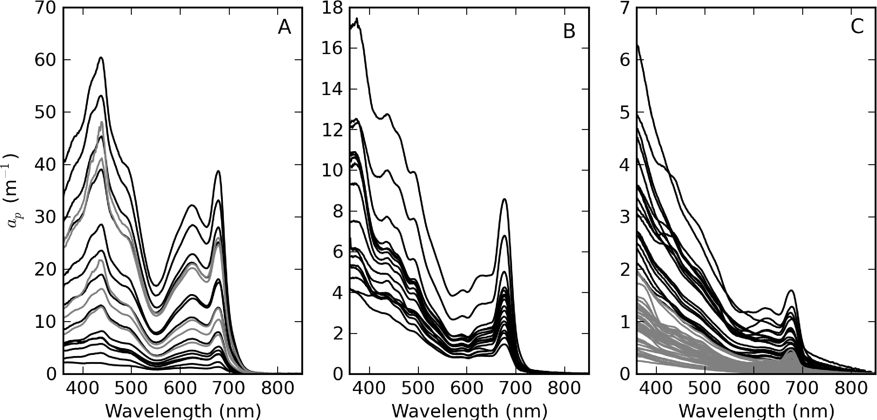
Figure 5 shows the measured ap spectra, which vary over more than four orders of magnitude. Extremely high ap values were measured in surface scum in Hartbeespoort (Table 2, Figure 5A). These spectra have shapes that indicate that the contribution of phytoplankton to ap is overwhelming. The spectra for Loskop are divided into two groups to facilitate comparison—the first is from the high biomass C. hirundinella bloom at sampling point CT (Figure 5B) and the second is from other sample points (Figure 5C). The spectra from point CT are strongly dominated by phytoplankton absorption, while the remainder have more exponential shapes, evidence of relatively larger tripton influence. ap spectra measured in Theewaterskloof (Figure 5C) appear to be influenced by significant contributions of both tripton and phytoplankton, with strong exponential shapes at wavelengths < 500 nm.
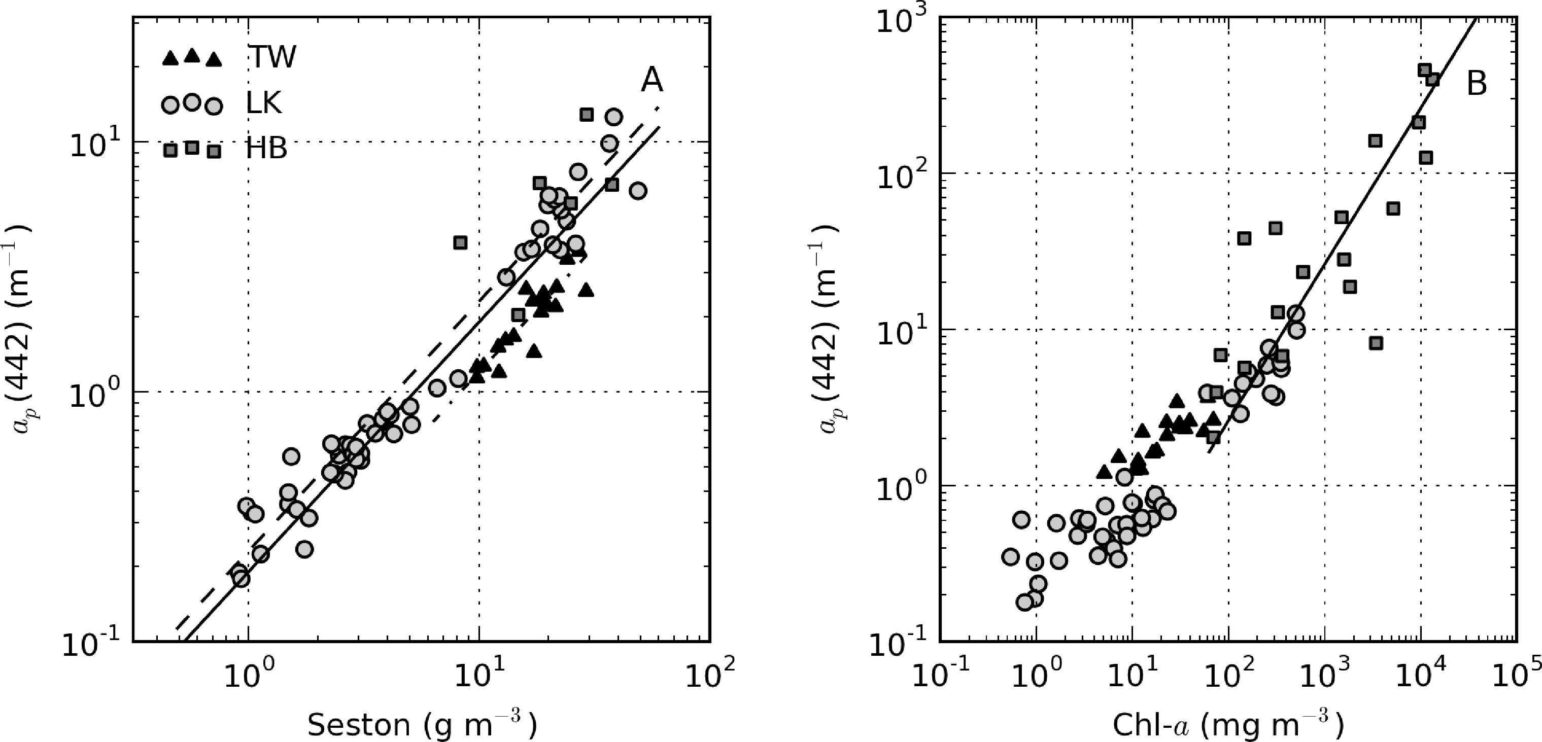
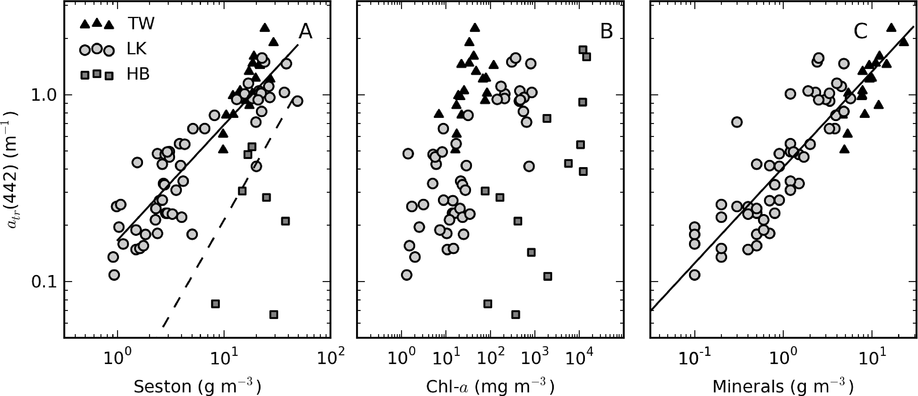
ap(442) is most variable in Hartbeespoort and Loskop (0.16–456.24 m−1) and was least variable in Theewaterskloof (1.13–3.65 m−1). ap(442) is highly covariant with seston and chl-a concentrations (Figure 6). A null intercept linear function (y = ax) was used to fit the data. The relationship ap(442) = 0.23 × seston was determined for Loskop (r2 = 0.91, SE (standard error)= 1.03, N = 56), similar to that determined for Theewaterskloof, ap(442) = 0.12 × seston (r2 = 0.97, SE = 0.38, N = 19). For combined Theewaterskloof and Loskop data, the relationship is ap(442) = 0.19 × seston (r2 = 0.85, SE = 1.22, N = 75). The variation in the regression coefficient, a, demonstrates the variability in the underlying IOPs. ap(442) was better described by chl-a in Hartbeespoort according to ap(442) = 0.026 × chl-a (r2 = 0.82, SE = 67.9, N = 19). The combined dataset was described by ap(442) = 0.15 × seston (r2 = 0.68, SE = 40.25, N = 91), and ap(442) = 0.026 × chl-a (r2 = 0.82, SE = 29.9, N = 94). The significance of the regressions is affected by the very high seston and chl-a concentrations in Hartbeespoort.
3.4. Absorption by Tripton
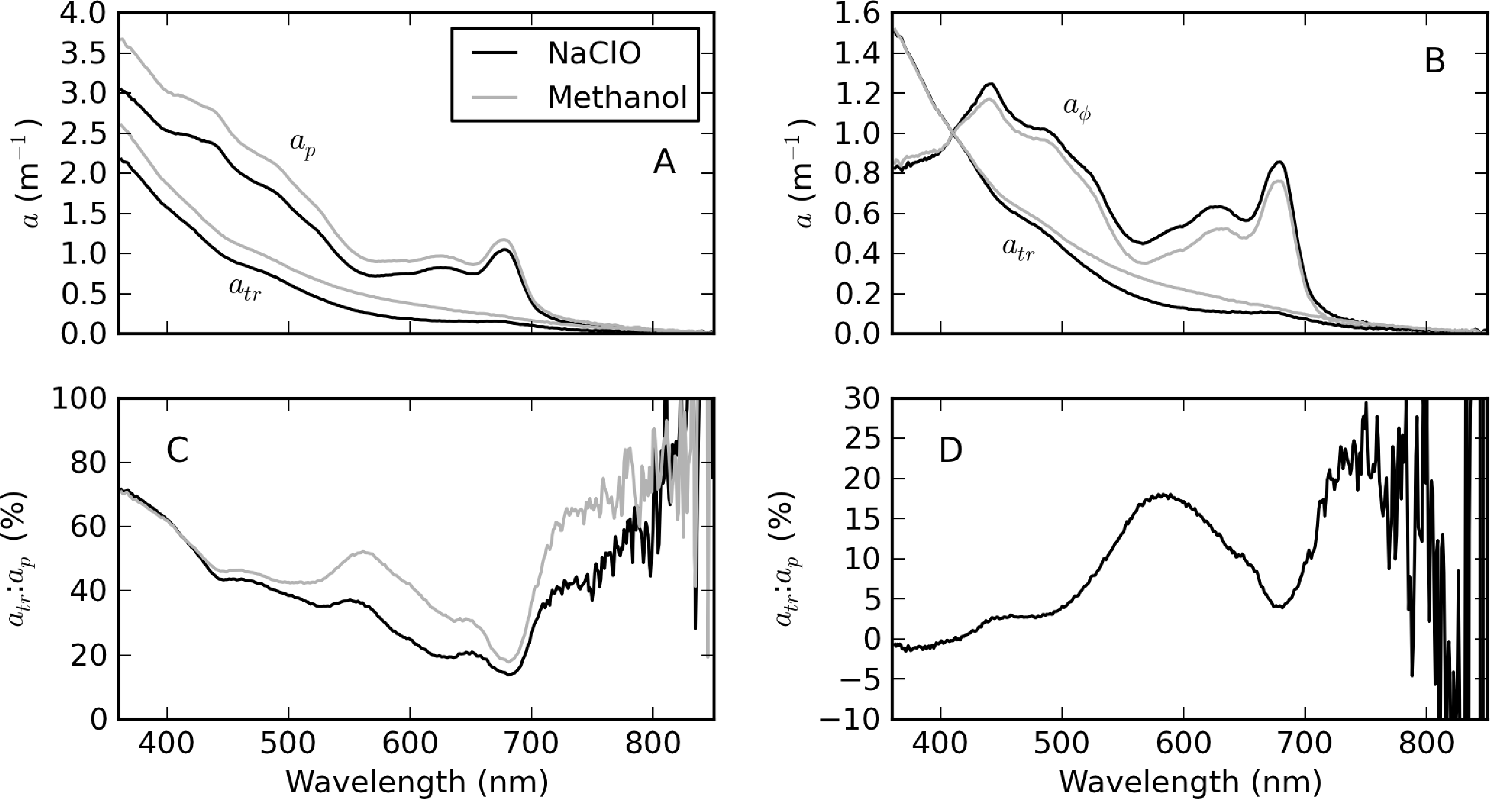
Figure 7 shows atr spectra from a single sample with a mixed cyanophyte/diatom/chlorophyte assemblage from Theewaterskloof determined by both hot methanol extraction and NaClO bleaching methods. The differences in magnitude of ap in Figure 7A are due only to the expected differences between duplicate samples. However, after normalizing at 410 nm (Figure 7B), appreciable spectral differences are present, as well as in the corresponding aph spectra. Although no apparent residual PC absorption peak at 620 nm is visible in the spectra, the methanol determined atr:ap ratio spectrum reveals that residual phycobilipigments are present in the region 500–650 nm, when compared to that determined by NaClO (Figure 7C). The difference between the atr:ap ratio spectra of the two methods shows that the hot methanol method leads to a 15%–20% underestimate of aϕ (or overestimate of atr) in the region between 500 and 650 nm (Figure 7D). The shoulders near 420 and 650 nm are likely associated with residual chl-b pigment from Chlorophyceae, which also results in a ±4% difference in the 675 nm chl-a absorption peak. Some evidence of bleaching of organic detritus by NaClO is visible from 700 to 750 nm (although not <440 nm), with both methods being roughly equivalent from 800 nm onwards. Therefore, in this example, the hot methanol technique resulted in residual phycobili and chlorophyte pigments in atr, while there was bleaching of organic detritus by NaClO in the near infra-red (NIR) region.
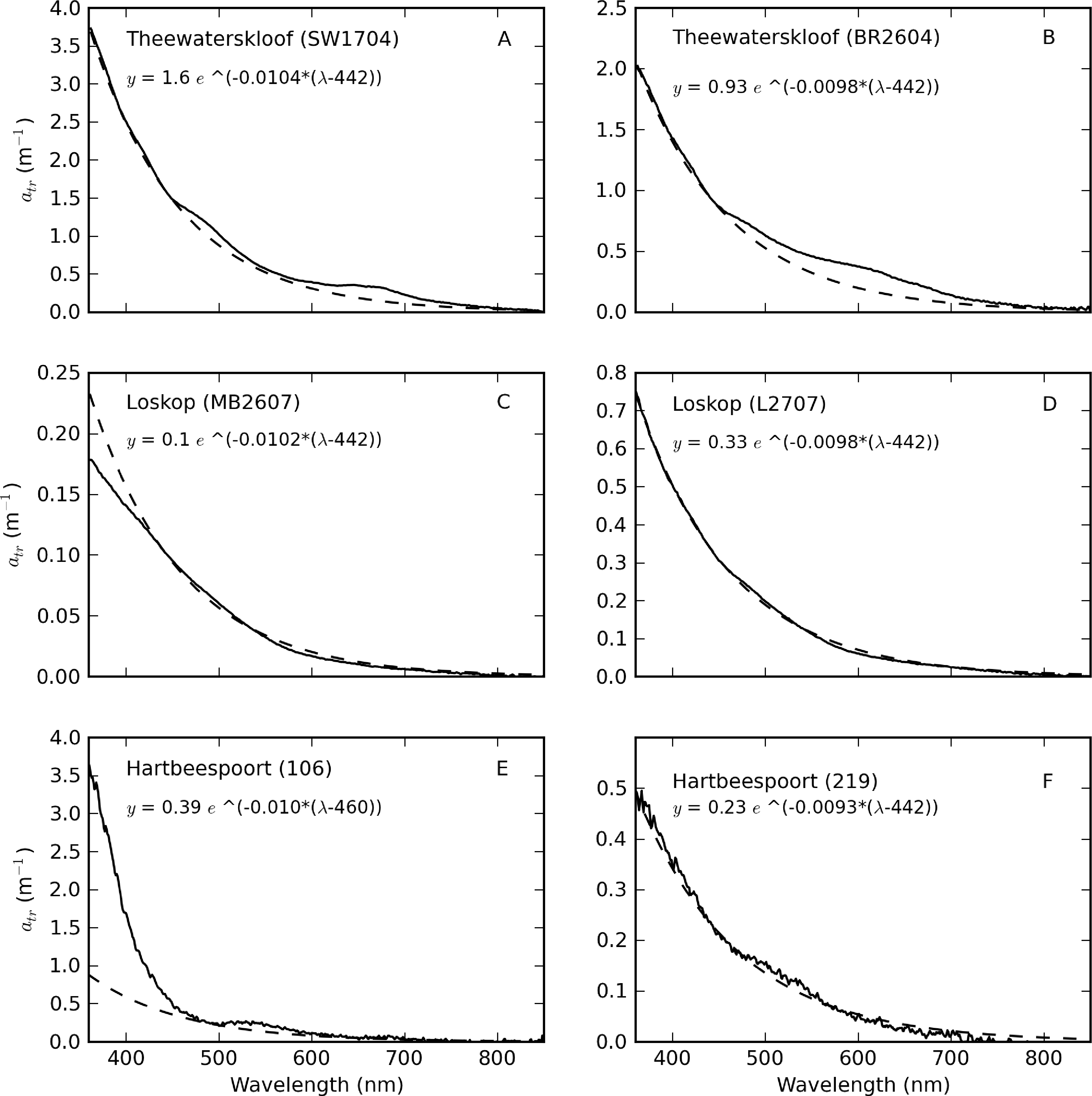
Some selected examples further illustrate these and other unusual features present in the measured atr spectra (Figure 8). In Theewaterskloof, a strong absorption feature near 450–550 nm, which is likely to be associated with iron oxides, was visible [52]; some residual chl-a absorption is also apparent (Figure 8A). In a few examples, residual phycobilipigment features were clearly visible (Figure 8B). To overcome this methodological error in the Theewaterskloof data, Str was calculated using an exponential function fitted between 360 and 500 nm. Another unusual feature was a flattening <440 nm for atr measured at point MB in Loskop (Figure 8C), the origin of which is unknown (see similar feature in Baltic spectra in [3]). For these data, an exponential function fitted between 440–600 nm was used to calculate Str. Iron oxide features (less obvious) were also present for some spectra in Loskop (Figure 8D). In Hartbeespoort, unusually steep slopes affecting wavelengths <450 nm were clearly visible (Figure 8E). Heterotrophic bacteria are known to be present in Hartbeespoort and other hypertrophic lakes in high abundance [53]. Therefore, the effect is likely to be caused by yellow cytochrome byproducts from NaClO bleaching, which are deposited on the filters [46]. All but two of the measured atr spectra in Hartbeespoort were contaminated by this effect. Therefore, Str was only computed for two uncontaminated spectra in Hartbeespoort, which also displayed some iron oxide effects (Figure 8F). Corrected atr spectra were computed by extrapolating the value at 460 nm using an exponential function with a slope coefficient = 0.009 nm−1. The extremely high biomass and the presence of heterotrophic bacteria in M. aeruginosa blooms in Hartbeespoort meant that determination of atr was challenging. Obvious residual phycobilipigment features were also sometimes present, resulting from inefficient NaClO bleaching. Therefore, determination of atr in hypertrophic waters or surface scum is perhaps better performed using a numerical technique (e.g., [44]). However, the contribution of tripton to ap was very small (see below).
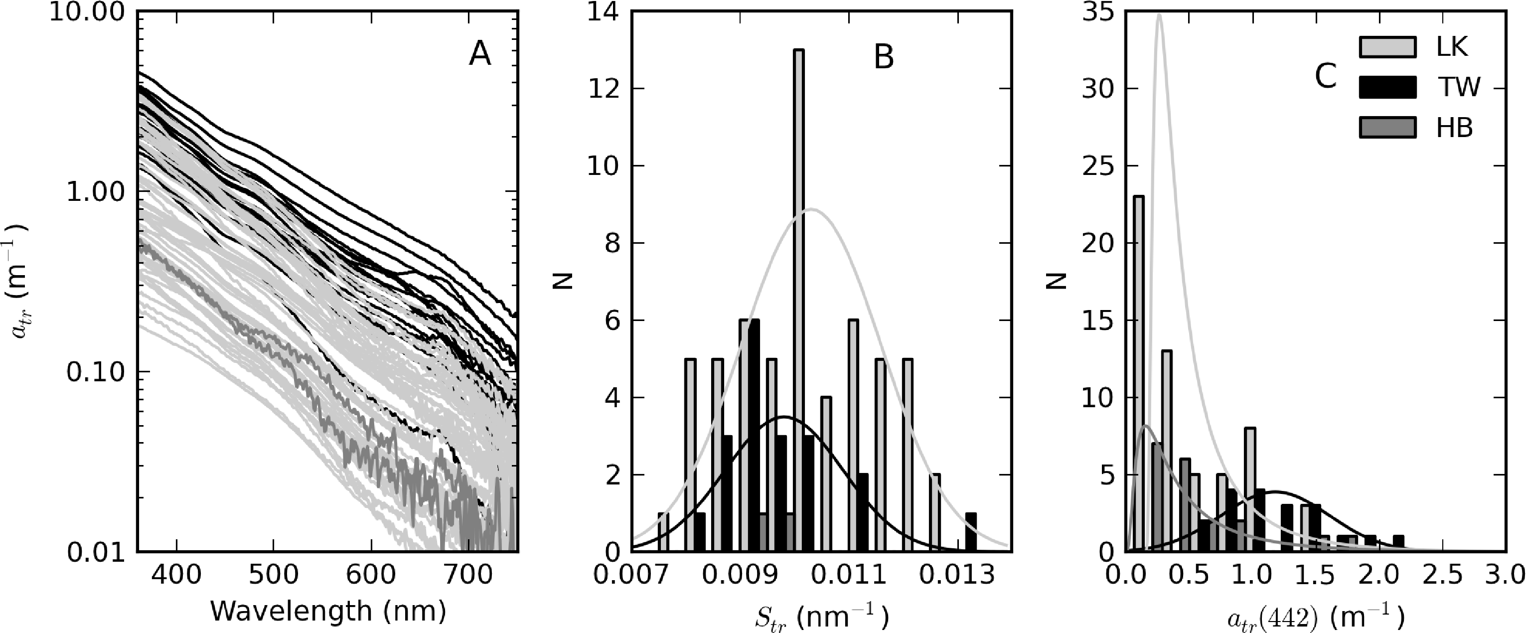
The complete set of measured atr curves are shown in Figure 9 alongside histograms for Str and atr(442). In general, an exponential function closely fitted the data, evident by the straight lines on the log-scale plot (Figure 9A). Of the three reservoirs, Theewaterskloof has the highest mean atr(442) value (=1.18 m−1), nearly twice that of Loskop and Hartbeespoort (see Table 1). atr(442) also has the highest range (= 1.75 m−1) in Theewaterskloof. This might be related to the high mineralic component of seston and the windy climatology of the reservoir. The range of atr(442) values for Hartbeespoort and Loskop are very similar (mean = 0.51 and 0.53 m−1, respectively), despite the extremely variable trophic conditions. This is because the variability in atr(442) is only weakly influenced by phytoplankton biomass (see below). The distributions of atr(442) for Hartbeespoort and Loskop are skewed towards smaller values and may generally be described by an inverse-Gaussian function (Figure 9C). Therefore, there is an increased probability of encountering atr(442) values < 0.5 m−1 in these systems, while it is also unlikely to encounter values >2 m−1. The Theewaterskloof data conforms more closely to a normal distribution with an increased likelihood of encountering atr(442) values near 1.0 m−1. The values determined for Str vary in a narrow range between 0.008 and 0.013 nm−1, with a mean value of 0.010 nm−1 for all reservoirs (Table 1, Figure 9B). These are typical of those measured in other inland and coastal waters (e.g., [3,9,37]). The distribution of Str generally follows the shape of a normal distribution; therefore, the highest probability value is near 0.010 nm−1.
atr(442) is significantly positively correlated with seston for Theewaterskloof and Loskop; the relationship is best described by a power-law fit as atr(442) = 0.17×seston0.62 (r2 = 0.81, N = 74) (Figure 10A). A null-point linear fit, such as those determined by Binding et al. [9] in lake Erie (drawn in Figure 10A) and Babin et al. [3] in European coastal waters, poorly describes the lower range of the data. In Hartbeespoort, the relationship is poor (r2 = 0.32, N = 16). This could result from errors in the corrected atr(442) values or methodological errors associated with atr determination in surface scum conditions. However, it may also be more simply explained by tripton making up an insignificant proportion of the dry weight, the majority of which is living cells. There is considerable scatter between atr(442) and TChl, which varies over six orders of magnitude (Figure 10B). Weak positive correlations are apparent within the reservoirs, indicating that trophic status weakly covaries with atr(442) within the systems. The significant offset for Hartbeespoort data indicates that in surface scum conditions, the tripton:phytoplankton ratio is significantly lowered. In contrast, the grouping of Theewaterskloof data towards the left of the plot is indicative of an enlarged tripton:phytoplankton ratio, in this case, presumably resulting from a higher mineralic component. Mineral (ash) dry weight and atr(442) are highly correlated with a fit for combined Loskop and Theewaterskloof data of atr(442) = 0.0.41×minerals0.51 r2 = 0.77, N = 70 (Figure 10C). The clustering of the Theewaterskloof data towards the top right of the plot is evidence of the high mineral content of seston (mean mineral contribution to seston = 57%). This may be a result of the high silica content of abundant diatom species.
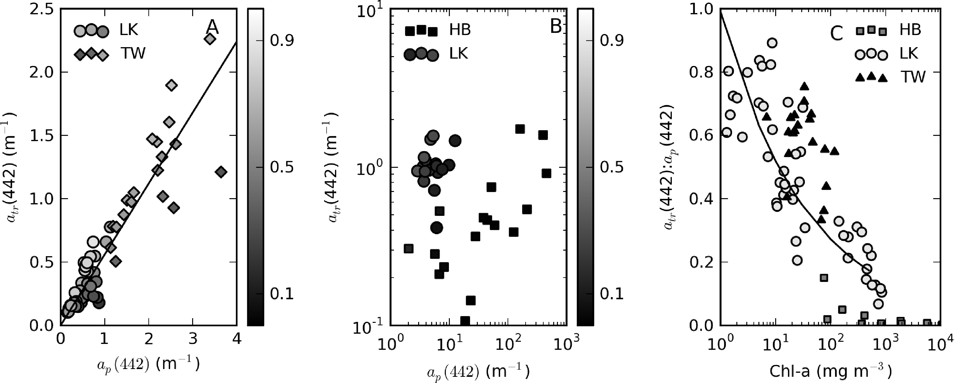
The variability in the contribution of tripton to ap between and within the reservoirs warrants closer investigation. For samples with ap(442) < 2, a positive linear relationship between atr(442) and ap(442) exists: atr(442) = 0.56 × ap(442), r2 = 0.94, SE = 0.2, N = 58 (Figure 11A). Mean atr(442):ap(442) ratios for these data are 0.65 for Theewaterskloof (range = 0.35–0.75) and 0.7 (range = 0.4–0.9) for Loskop. Tripton, therefore, has a large contribution to particulate absorption for these data. For high biomass Loskop and Hartbeespoort waters, the relationship between atr and ap breaks down (Figure 11B). In these waters, atr is an insignificant contributor to ap, with atr(442):ap(442) ratios of 0.1–0.35 in Loskop and <0.15 in Hartbeespoort. When investigating the change in the atr(442):ap(442) ratio relative to phytoplankton biomass (TChl), we find a general inverse correlation, which is specific to each lake (Figure 11C). In Loskop, the relationship is described by atr(442):ap(442) = 0.99 × TChl−0.28 (r2 = 0.76, N = 47), while in Hartbeespoort, it is atr(442):ap(442) = 0.37 × TChl−0.50 (r2 = 0.62, N = 14). In Theewaterskloof, the relationship was much weaker (r2 = 0.2 for a linear fit), signifying that phytoplankton biomass does not dictate the contribution by tripton to particulate matter. Evidently, tripton typically contributes more towards ap(442) as phytoplankton biomass decreases. Therefore, phytoplankton biomass exerts a controlling influence on the contribution that tripton makes to particulate absorption (although less so for Theewaterskloof). The converse effect is visible in a weak positive correlation between minerals and the atr(442):ap(442) ratio (not shown). There is no apparent relationship between the ratio and seston concentration.
3.5. Mass-Specific Tripton Absorption
The chl-a content of seston (chl-a:seston ratio) might be used to test for steady state conditions [36]. Figure 12A shows the mean chl-a:seston ratio determined for different sample points in Loskop and for Theewaterskloof and Hartbeespoort as a whole. Non-steady-state conditions were indicated by widely variable ratios at point CT in Loskop (6–18 mg·g−1) and in Hartbeespoort (4–11 mg·g−1). Variability elsewhere was relatively small. Therefore, non-steady-state conditions are associated with the high biomass blooms in Loskop and Hartbeespoort. Rpd is, therefore, expected to be larger than 0.3 in these blooms, but should be near 0.3 elsewhere, regardless of the trophic state.
The Rpd values calculated using β ranging between 0.01–0.1 g·mg−1 and averaged by the sample point/reservoir are shown in Figure 12B. For steady-state Loskop sample points, BY (buoy), LS and MB, values of β corresponding to Rpd ≈ 0.3 are approximately 0.04, 0.055 and >0.1 g·mg−1, respectively. By choosing a single value of β = 0.04 g·mg−1 for Loskop, the corresponding Rpd values become 0.29, 0.20 and 0.04. This is in the acceptable range of values encountered in steady-state conditions considering that chl-a at point MB was very small, >1 mg·m−3. The value determined for β is lower than the mean value for C. hirundinella (=0.079 g·mg−1 [39]), but is within the lower range determined for natural populations of flagellates (=0.037–0.714 g·mg−1 [38]). Assuming the same value for β can be used for the bloom at point CT, the corresponding Rpd is 1.3. Such a high value might be acceptable, since negative Rpd values are observed for β values > 0.05 g·mg−1 at point CT. This is a result of phytoplankton dry mass calculated using β exceeding seston dry weight.
Because of the difficulty in measuring parameters in surface scum conditions, only samples with chl-a < 500 mg·m−3 were used in the calculations. The value for β determined in Hartbeespoort is approximately 0.03 g·mg−1 (Figure 12B), just under the range of 0.033–0.769 g·mg−1 determined by Desortová [38] for blue-green assemblages. However, a Rpd value of 0.3 is likely too low for the non-steady-state bloom conditions. The average literature value of for M. aeruginosa = 0.09 g·mg−1 [37,39] gives a Rpd = 1.83 (one negative value was removed from the calculations, N = 17). This Rpd is similar to that obtained at point CT in Loskop. Theoretically, however, β could lie anywhere between 0.03 and 0.09 g·mg−1 in Hartbeespoort. In Theewaterskloof, a β value of 0.09 g·mg−1 was determined. This is close to literature values for Anabaena = 0.063 g·mg−1 and lower than those for diatoms Asterionella and Aulacoseira (β= 0.18 and 0.12 g·mg−1) [39], both of which are present in Theewaterskloof. In summary, β values for Loskop, Hartbeespoort and Theewaterskloof were finally chosen as 0.04, 0.09 and 0.09 g·mg−1, respectively.
The (442) values determined using the aforementioned β values are shown in Figure 12C, and the mean spectrum for each reservoir in Figure 12D. (442) ranges from 0.025 to 0.263 m2·g−1 in Loskop, 0.054 to 0.105 m2·g−1 in Theewaterskloof and from 0.024 to 0.048 m2·g−1 in Hartbeespoort. The mean values are 0.119, 0.078 and 0.037 m2·g−1, respectively. These values compare favorably with those reported in other fresh inland waters (e.g., [6,33,37]). In particular, values of (550) for various lakes in Queensland Australia varied between 0.014 and 0.145 m2·g−1 [6]. The mean spectrum for Theewaterskloof is evidently mineral-rich and affected by iron oxide absorption effects near 500 nm. The specific absorption coefficients of terrigenous mineral-rich particulate matter vary over a wide range from <0.1 to 1 m2·g−1 (e.g., [54,55]). Therefore, the values determined here appear to be consistent within the variability present in the literature. A brief investigation of the sensitivity of (442) to the value of β shows that in Hartbeespoort, mean (442) values produced by β of 0.03 and 0.09 g·mg−1 are 0.0145 and 0.0374 m2·g−1, respectively. Therefore, the value of β has an appreciable influence on (442) and should, therefore, be chosen with care, for example, using the method presented here.
3.6. Absorption by Phytoplankton
aϕ for Theewaterskloof was calculated without correcting the atr spectra for residual phycobilipigment, because of the strong iron oxide absorption feature. Therefore, aϕ may be underestimated by a maximum of 15% in the region 550–650 nm for these data. In the case of Hartbeespoort, an exponential function with slope Str = 0.010 (the mean value determined for uncontaminated spectra) was used with the value of atr determined at 460 nm to calculate aϕ. This was because atr was contaminated by NaClO bleaching of heterotrophic bacteria. As the contribution to ap by tripton was so small relative to phytoplankton (see Figure 11), the effect of this correction on aϕ is insignificant.
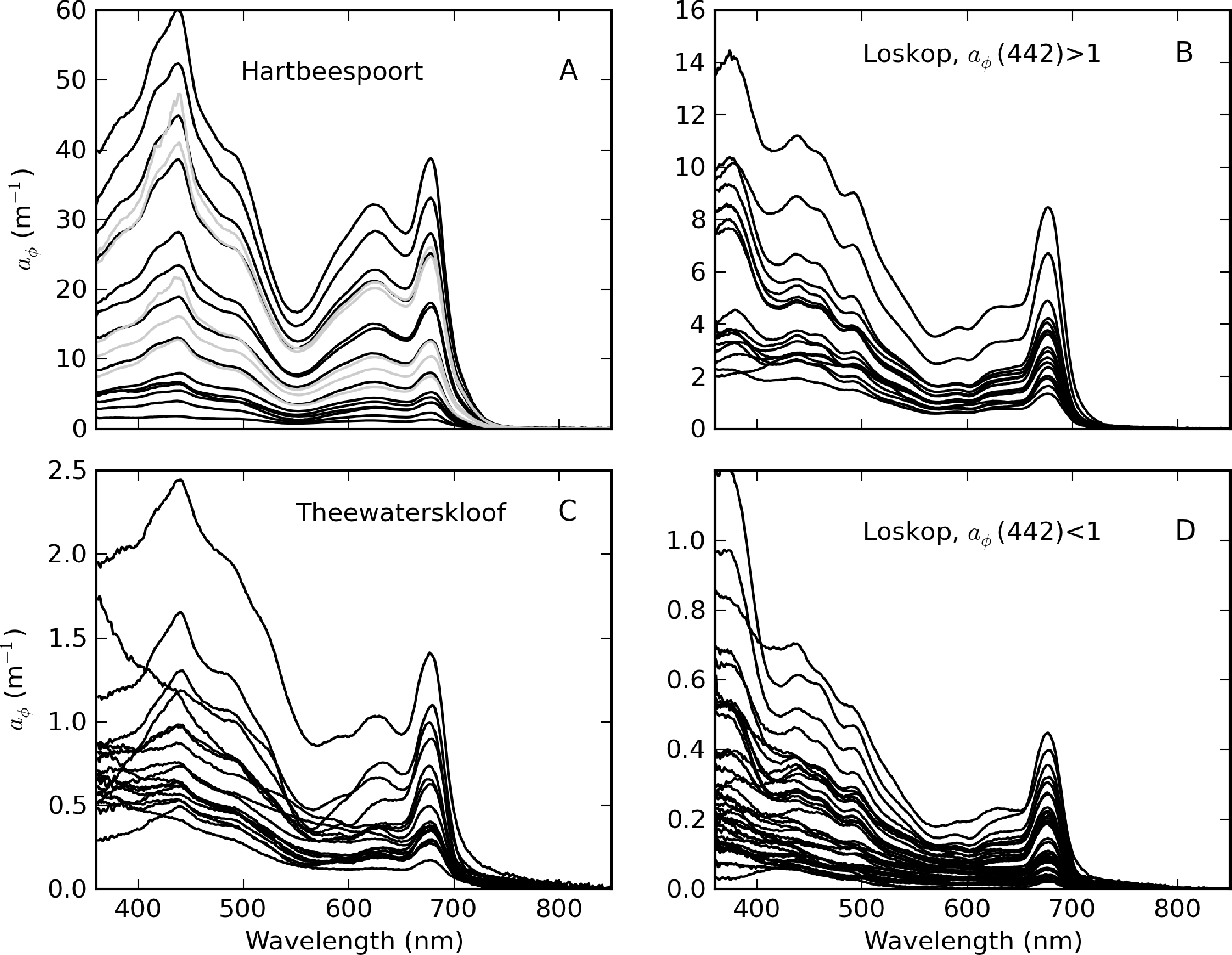
The diversity of trophic states and phytoplankton assemblages between and within the reservoirs was evident in aϕ spectra that vary widely in shape and magnitude (Figure 13). Extremely high aϕ values > 400 m−1 were measured in M. aeruginosa surface scums in Hartbeespoort (Figure 13A). The spectral shapes have typical chl-a absorption peaks along with strong phycobilipigment features between 550–650 nm (phycocyanin and phycoerethrin) and shoulders associated with the carotenoids myxoxanthophyll, zeaxanthin and echinenone (400–500 nm) [56,57]. The spectra from Loskop are much smaller in magnitude, with significantly different pigmentation features associated mainly with C. hirundinella. These have absorption shoulders in the region 400–500 nm from chlorophylls c1 + c2 (440 nm), the carotenoids, peridinin (460 nm) and, possibly, fucoxanthin (440–460 nm), and xanthophylls (diadinoxanthin, diatoxanthin) [57]. The presence of UV photoprotective mycosporine-like amino acids (MAAs) typical of dinoflagellates is strikingly evident < 400 nm [58]. aϕ spectra from Theewaterskloof have a mix of dinoflagellate and cyanobacterial pigment absorption features, both species being co-dominant. These and other features are described further in Figure 14.
Five of the aϕ spectra for Loskop determined using NaClO bleaching had shapes that increased exponentially towards the blue. These spectra were associated with low chl-a values (<1 mg·m−3) and relatively high gelbstoff concentrations (ag(440) = 0.94–1.5 m−1). It is possible that this affect may be caused by NaClO bleaching of dissolved organic matter (DOM) in the presence of relatively high gelbstoff absorption [9]. However, because of the presence of a strong signal from MAAs < 400 nm, it is difficult to ascertain whether bleaching did in fact occur (see Figure 7). For example, a similar effect was also visible in two spectra from Theewaterskloof. Since these were determined using boiling methanol, the effect cannot be caused by NaClO bleaching and is probably better attributed to accessory pigments (MAAs), methodological errors or an unknown source. There was no further evidence of bleaching of DOM by NaClO.
3.6.1. TChl-Specific Phytoplankton Absorption
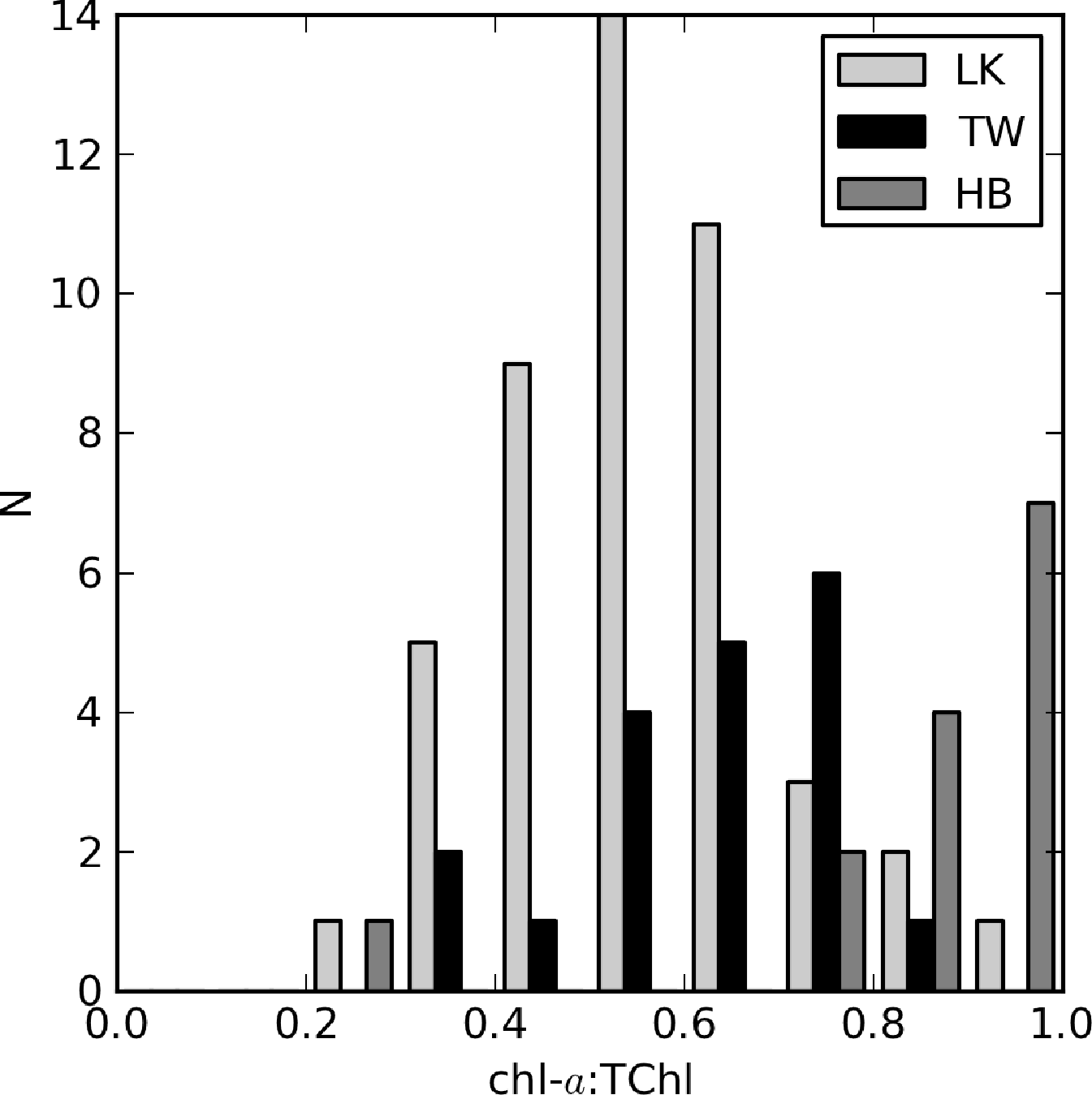
The relationship between aϕ(440) and TChl is affected by pigment packaging (cell size) and accessory pigments, the former of which has the greatest effect [4,59]. In Case 1 ocean waters, there is a general relationship between cell size and trophic state, with larger cells occurring at higher TChl values. Therefore, the aϕ to TChl ratio (or the specific absorption ) decreases with increasing TChl, due to pigment packaging, which is manifest by an exponential relationship between aϕ and TChl. Similarly, the influence of non-photosynthetic pigments relative to chl-a, measured as the ratio of blue to red phytoplankton absorption, tends to decrease as TChl increases. This also contributes to the effect. However, in coastal waters, accessory pigments, such as phaeopigments and phytoplankton size dynamics, are responsible for large variations in aϕ (e.g., [3,60]). The influence of phaeopigments is significant in both Loskop and Theewaterskloof (chl-a:TChl ≈ 0.5 and 0.7, respectively) and less so in Hartbeespoort (Figure 15). Therefore, it is expected that variable accessory pigments and size will also cause large variations in aϕ in lakes.
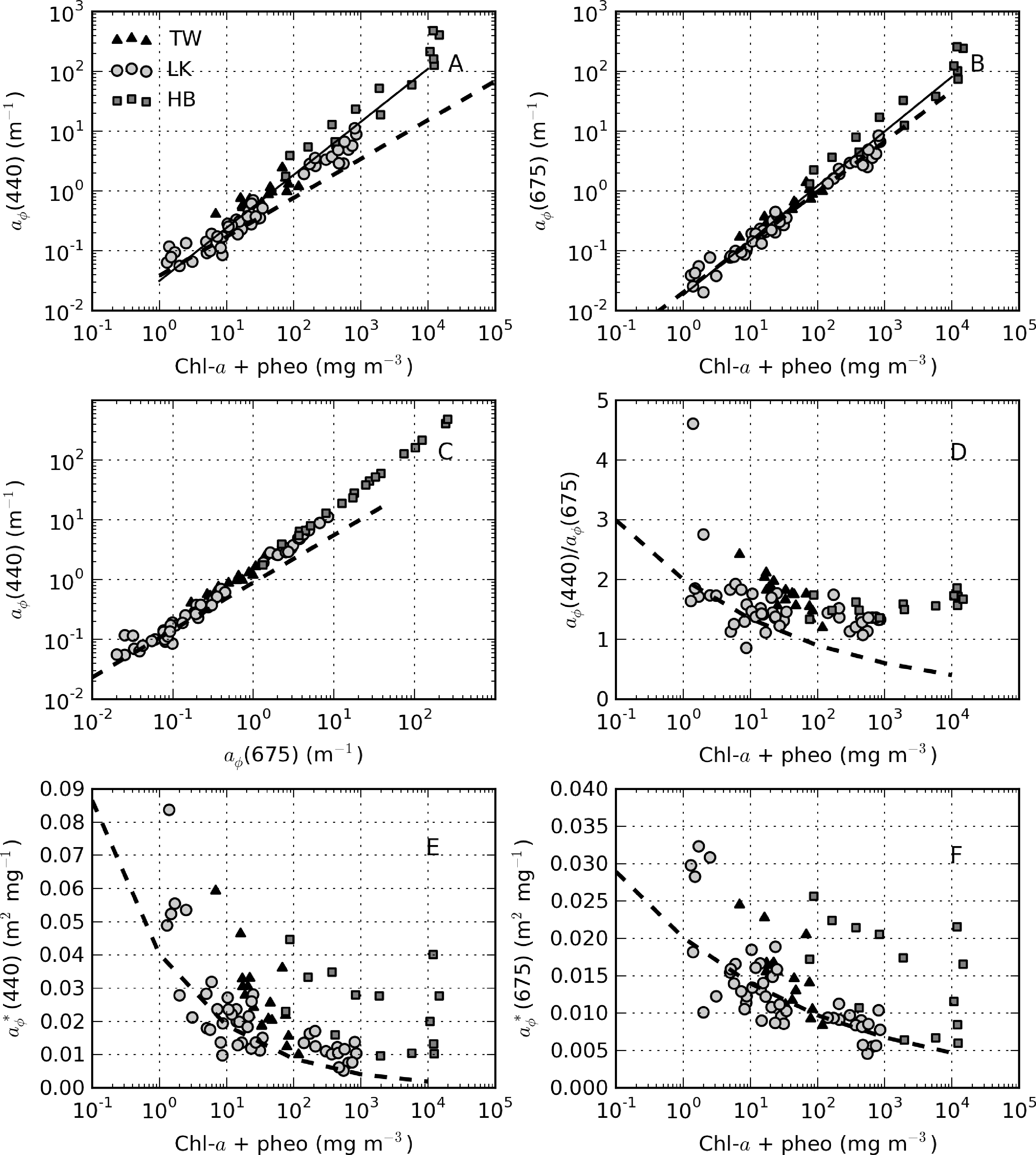
Figure 16A shows the relationship between aϕ(440) and TChl, which is best described by aϕ(440) = 0.031TChl0.89 (r2 = 0.95, N = 82). For TChl < approximately 30 mg·m−3, the data are in general agreement with Case 1 estimates, after which they are positioned above the extrapolated line (maximum TChl value in Bricaud et al. [4] = 25 mg·m−3). The reasons for the deviation are most easily explained by looking at each reservoir in turn. In Loskop, the explanation is not likely related to cell size (the package effect), since the dominant species is the large-celled C. hirundinella. A more plausible explanation is the presence of strong accessory pigments (Figure 15). The aϕ blue:red ratio decreases only slightly with increasing TChl values (Figure 16C,D), evidence of significant accessory pigment influence at high TChl values. This is not inside expectations for typical Case 1 waters. For aϕ(675), however, the data are in close agreement with Bricaud et al. [4], where the influence of accessory pigments is reduced (aϕ(675) = 0.018TChl0.91, r2 = 0.97, N = 82) (Figure 16B). Therefore, accessory pigments are the cause of large deviations from Case 1 results in the blue spectrum. The same explanation might be given for the same effect observed for Theewaterskloof data, since the phytoplankton assemblage is also generally dominated by a mix of large-celled species.
It is apparent in Figure 15A,B that the Hartbeespoort data are consistently above those of Theewaterskloof and Loskop. Accessory pigments alone cannot explain this large deviation from classical Case 1 results. A more likely cause is the small cell size of the dominant species, M. aeruginosa (d = 5 μm), leading to reduced pigment packaging. Although M. aeruginosa exists in colonial aggregations of large size, the affect on the bulk IOPs appears to be consistent with small cells. Despite the extremely high TChl values, accessory pigments also appear to have a significant impact in blue wavelengths (Figure 16C,D). Therefore, it is apparent that the M. aeruginosa blooms violate both of the assumptions of Case 1 waters, especially that cell size increases with trophic state. This is also likely to be the case for many other fresh waters dominated by small-celled cyanobacteria, resulting in wide inter- and intra-lake variability in . The corresponding versus TChl scatter plots demonstrate this variability (Figure 16E,F). (440) values are expectedly larger than those typically observed in Case 1 waters; however, the agreement is better for (675) (for the reasons given above). The increase in induced by small cell size is evident for Hartbeespoort. The wide ranging values for TChl > 1,000 mg·m−3 might be a result of the difficulty of measuring both absorption and TChl in ”scum” conditions—methodological errors are prone to become greatly enlarged in both techniques. The lake-specific exponential fits for versus TChl are shown in Table 4.
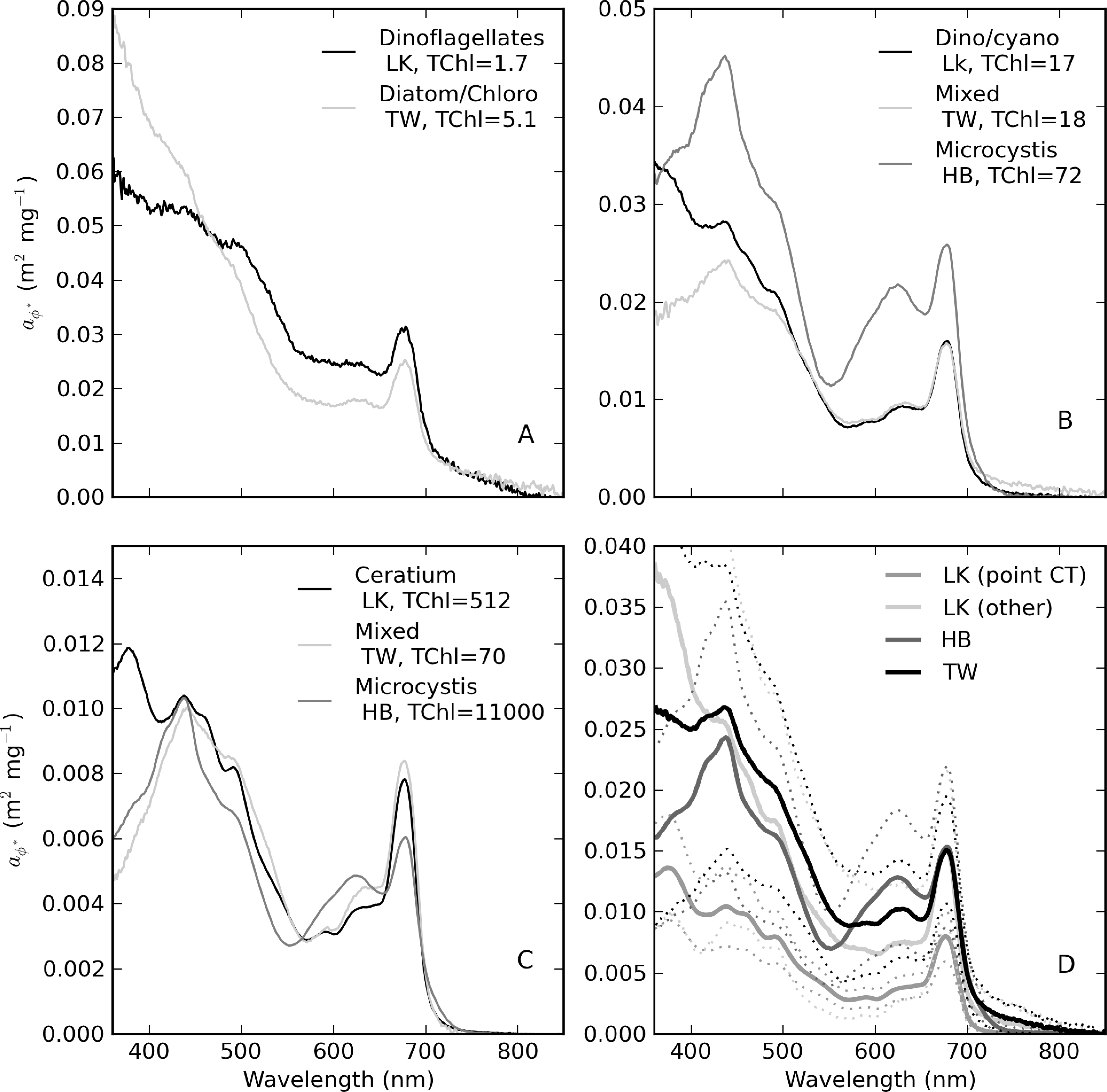
Figure 14 provides selected examples of spectra arranged by trophic class, as well as the mean for each reservoir. Table 5 gives statistics for (440) arranged by trophic class, as well as for the M. aeruginosa and C. hirundinella monospecific blooms. The statistics show that the mean value of (440) decreases from oligotrophic to hypertrophic classes (from 0.056 to 0.018 m2·mg−1), in agreement with expectations. The variability (indicated by the standard deviation) also decreases with TChl (excluding the Hartbeespoort M.aeruginosa data). spectra from oligotrophic waters have spectra that occasionally slope upwards towards the blue (Figure 14A). This effect is likely related to strong accessory pigments at low TChl concentrations or possible DOM bleaching, in the case of Loskop. Meso-eutrophic waters associated with Loskop and Theewaterskloof typically have (440) values near 0.02 m2·mg−1 and similar shapes, due the presence of large-celled dinoflagellates in both reservoirs (Figure 14B). Figure 14C,D shows large differences in magnitude and spectral pigmentation for the C. hirundinella and M.aeruginosa blooms (mean (440) = 0.011 and 0.024 m2·mg−1, respectively). The wide variability of (440) for M. aeruginosa is most likely due to measurement difficulties associated with the extremely high biomass. These data represent the extrema of dinoflagellate and cyanobacteria dominance. The high variability in is related to the wide trophic range and variable phytoplankton populations in and between the reservoirs. This highlights the difficulty of applying generalized IOP models to lakes and the need for lake-trophic class and/or species-specific IOPs.
3.6.2. Phycocyanin-Specific Phytoplankton Absorption
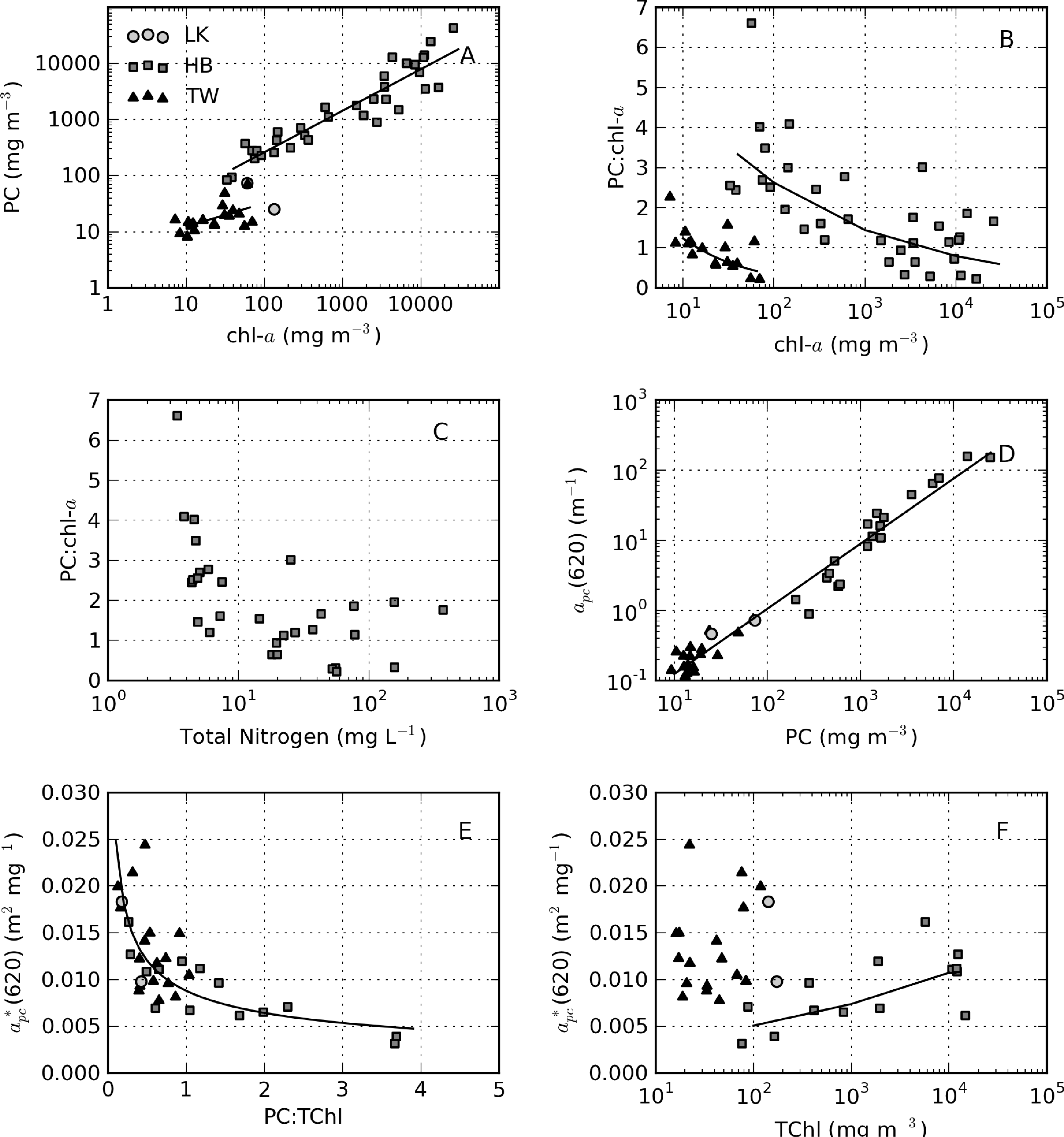
Phycocyanin pigment was determined for samples where cyanobacteria made up a significant proportion of the phytoplankton population. PC might give a better indication of cyanobacterial biomass than chl-a, given that it is the primary light harvesting pigment in cyanobacteria [61]. It is also a very distinctive pigment that may be used to discriminate cyanobacteria from other algal populations [62]. The relationship between PC and chl-a is best described by PC = 8.7 × chla0.74 for Hartbeespoort (r2 = 0.87, N = 34) and PC = 4.70 × chla0.4199 for Theewaterskloof (r2 = 0.32, N = 19) (Figure 17A). The Theewaterskloof data are from a mixed algae/cyanobacteria population. Therefore, chl-a originates from algae, as well as cyanobacteria, resulting in a reduced PC:chl-a ratio, as observed in Figure 17A. In contrast, the Hartbeespoort data are from a monospecific M. aeruginosa bloom. These data demonstrate that as cyanobacterial biomass increases, the production of PC is reduced relative to chl-a. A similar effect is observed in Hartbeespoort for accessory pigments allophycocyanin (APC = 11.2 × chla0.59, r2 = 0.68, N = 34) and pheophytin (Pheo = 0.16×chla0.9522, r2 = 0.95, N = 38). Accessory pigments are modulated either by high light and nutrient exposure (e.g., [63]) or through other physiological processes reflected by changes in gross biomass.
The equations for the PC:chl-a ratio versus chl-a were derived mathematically from the power-law function and are, therefore, not a result of “spurious correlation” [64]. According to the relationship, 8.7chla−0.26 (Figure 17B), the PC:chl-a ratio decreases from three at chl-a = 100 mg·m−3 to 0.7 at chl-a = 10,000 mg·m−3 in Hartbeespoort. This effect might be related to nitrogen limitation as cell abundance increases [65]; however, nutrient data acquired simultaneously reveal no shortage of total nitrogen (or other nutrients) associated with reduced PC:chl-a ratios (Figure 17C). An alternative explanation is that phycobilipigment production is reduced in high light, shallow mixed surface scum layers [63,66] or in fast growth scenarios. While a precise explanation for this effect remains somewhat unknown, the observation has some important implications for extremely high biomass and surface scum scenarios. If the production of accessory pigment PC is reduced relative to chl-a in surface scums, then chl-a might be a better indicator of biomass in these extreme conditions. Secondly, when interpreting measurements made in surface scums, the reduced accessory pigment production might be used to explain some unusual effects in the PC-specific absorption.
apc(620) and PC are related by apc(620) = 0.0146 × PC0.929 (r2 = 0.97, N = 36). Clustering in the data around 10–20 mg m−3 PC resulted in a reduced coefficient of determination for Theewaterskloof alone (r2 = 0.61), while PC varies by more than three orders of magnitude in Hartbeespoort (r2 = 0.93). The reduced goodness of fit in Theewaterskloof is likely the result of a strong influence near 620 nm of chl-c and chl-b from diatoms and chlorophytes. This is substantiated by relatively low PC:TChl ratios in Theewaterskloof (median = 0.53, see Figure 17E). An inverse relationship is present between the PC:TChl ratio and (620) (y = 0.0088x−0.451, r2 = 0.63, N = 31, Figure 17E), similar to that observed by Simis et al. [12]. The variability in (620) is typically attributed to the contribution of cyanobacteria to the total phytoplankton population [48]. While this is probably the case for Theewaterskloof, the variability observed in Hartbeespoort can only be caused by biomass related variable accessory pigment (PC) production. Therefore, (620) varies not only according to the relative contributions of cyanobacteria/algae, but also with physiological processes related to biomass affecting the PC:chl-a ratio within monospecific blooms (Figure 17B). Figure 17F provides some further evidence for biomass-induced changes in (620) in Hartbeespoort. A positive correlation is present between TChl and (620) (y = 0.0024x0.1627, r2 = 0.48, N = 14). No such relationship is apparent for Theewaterskloof. Therefore, the variability in (620) in Hartbeespoort appears to be caused, at least partially, by biomass-related phenomena related to reduced PC production in high light surface scum conditions.
The value for in vivo(620) was recently experimentally determined as 0.007 m2·mg−1 for a wide variety of cultured cyanobacteria [67]. The median values for (620) determined in Theewaterskloof and Hartbeespoort are 0.0122 and 0.0085 m2·mg−1, respectively. This is within the range of those previously measured in natural populations [12]. For PC:TChl ratios > 0.5 the value in Theewaterskloof is reduced to 0.010 m2·mg−1. For Hartbeespoort data not affected by large biomass effects, i.e., TChl < 1,000 mg·m−3, the median value for (620) is 0.0067, and the mean is 0.0072 m2·mg−1, which is nearly identical to that of Simis et al. [48] and Simis and Kauko [67]. This also demonstrates that the method for PC extraction used in this study is probably efficient.
3.7. Absorption Budgets
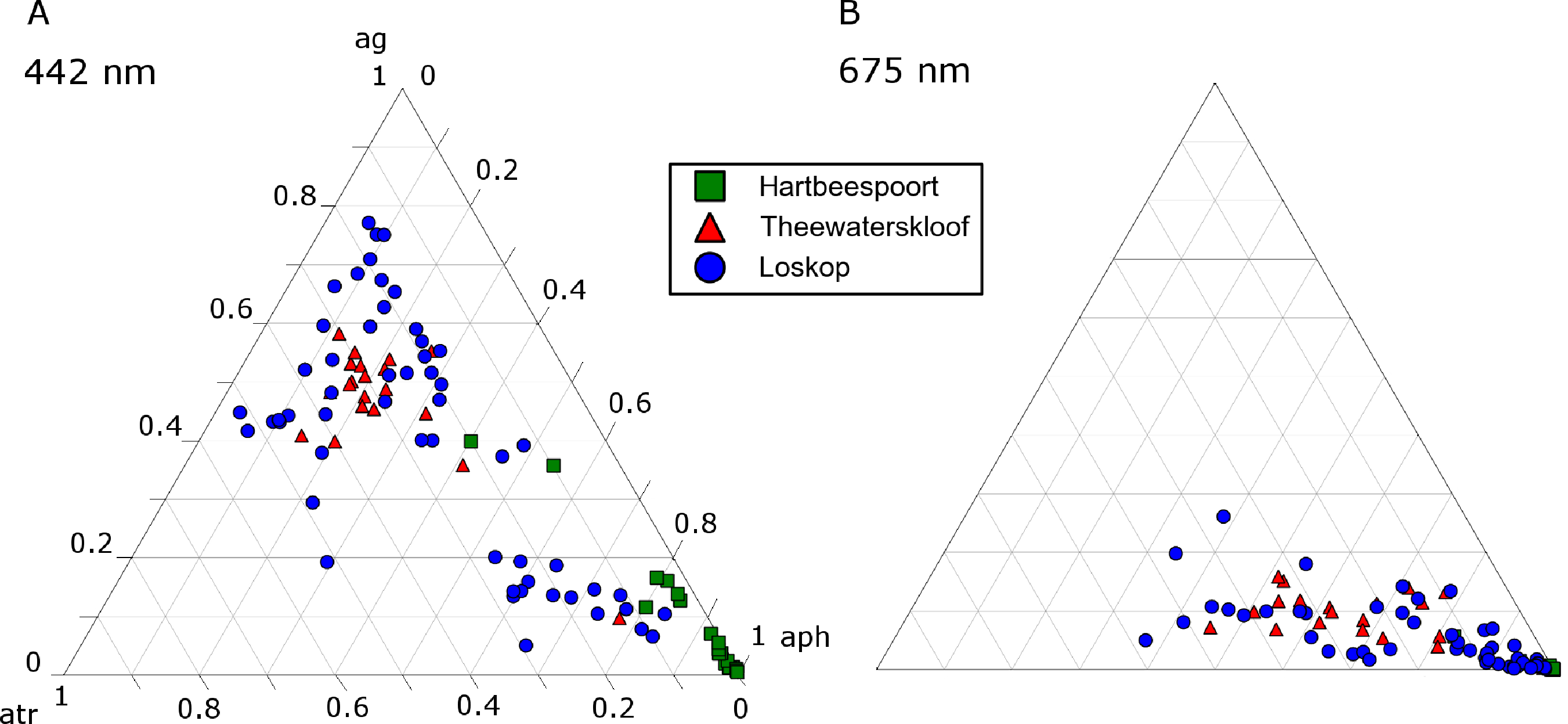
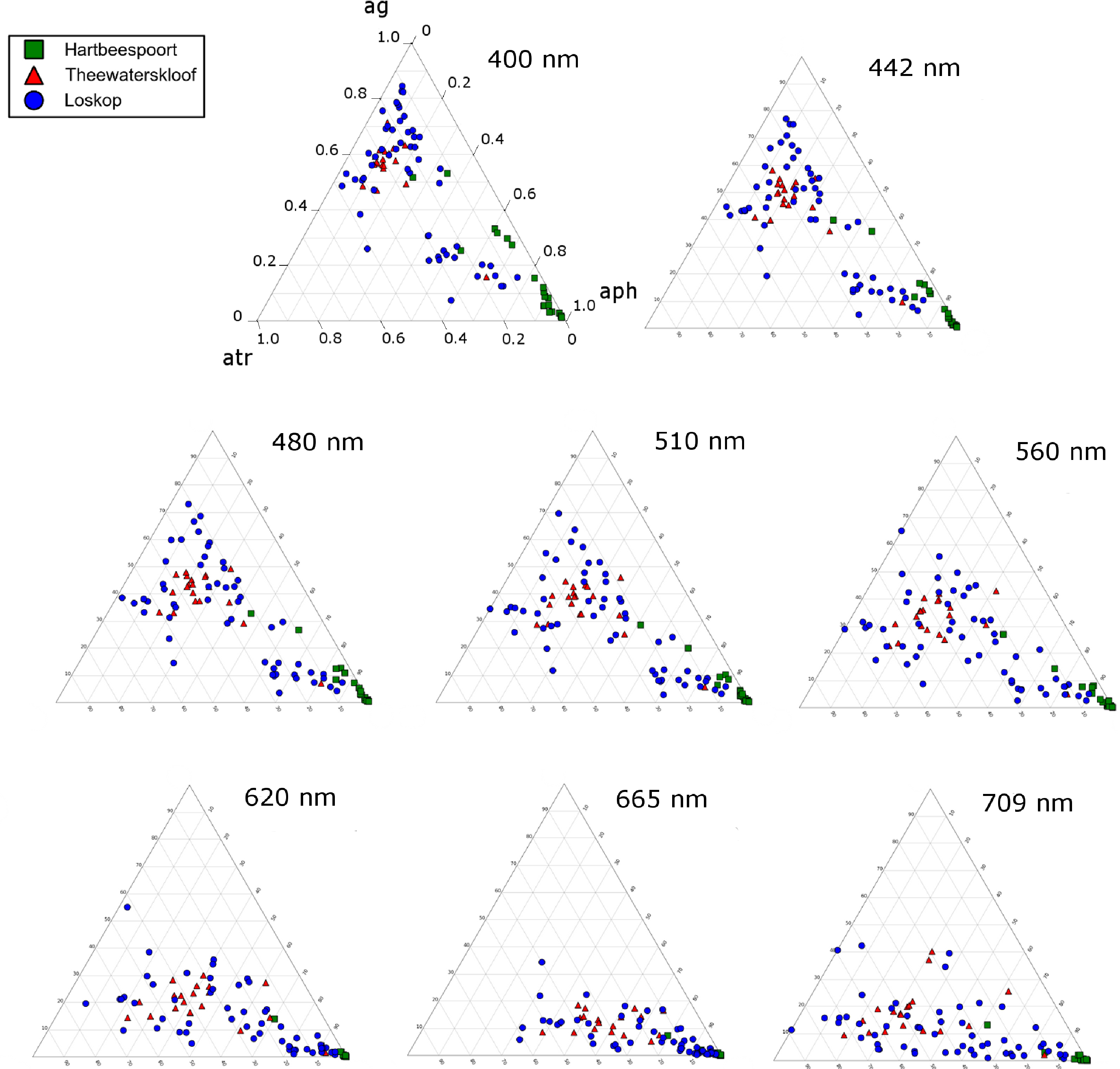
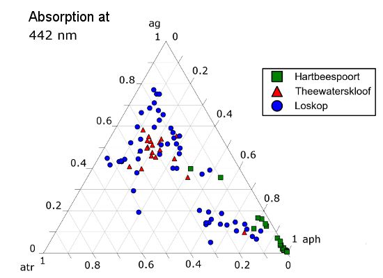
The ternary plots in Figure 18 show the relative contributions by gelbstoff, phytoplankton and tripton towards the total absorption budget of each reservoir. At 442 nm (Figure 18A), there is a strong influence by all components. The clustering of data from Hartbeespoort towards the phytoplankton apex is indicative of an overwhelming dominance of phytoplankton absorption. Therefore, Hartbeespoort waters (or the M. aeruginosa bloom) might strictly be classified as Case 1, i.e., phytoplankton are the dominant contributor to absorption [68]. Similarly, the cluster of Loskop data from the C. hirundinella bloom towards the phytoplankton apex might also be classified as Case 1: more than 80% of the absorption is attributed to phytoplankton. It should be noted, however, that while strictly speaking, these can be classified as Case 1 waters, the reflectance features of Case 1 green waters described by Morel and Prieur [68] will be substantially different to those described here. This might mean that some complexities regarding remote sensing applications are removed, and the blooms of M.aeruginosa and C. hirundinella can essentially be treated as ”cultures”, (i.e., the minimal influence of constituents other than phytoplankton). This provides an opportunity for remote sensing algorithms that take advantage of a signal originating primarily from phytoplankton in eutrophic waters. One such example is the maximum peak height algorithm [62] designed for use with the Medium Resolution Imaging Spectrometer (MERIS) red wavebands, which is derived from datasets obtained from Hartbeespoort and Loskop.
The remainder of the Loskop data is typically dominated by gelbstoff (40%–80%) with lesser contributions from phytoplankton (<50%) and tripton (20%–50%) towards absorption. Absorption in Theewaterskloof is generally comprised of 50% gelbstoff, 20% phytoplankton and 30% tripton. These fall into the classification of Case 2 or optically complex waters. At 675 nm, Figure 18B, the data are expectedly clustered towards the phytoplankton apex, which results from the reduced influence of tripton and gelbstoff absorption in red wavelengths. This shift due to the spectral characteristics of the absorption components is visible at various wavebands of the upcoming Sentinal 3 and past MERIS sensors (Figure 19). The majority of the water encountered in the reservoirs are complex from an optical perspective, requiring remote sensing applications, taking into account the absorption characteristics of all water constituents presented here. A recent study by Matthews and Bernard [14] demonstrates an approach utilizing IOPs derived from this study for radiative transfer modeling and the derivation of remote sensing algorithms.
The analysis conducted here is based on sampling campaigns conducted over a short time period and at various times of the year. There is significant seasonal variability in the contribution of phytoplankton towards the absorption budgets, with the maximum being reached in later summer and the minimum during winter (Matthews, unpublished data). This has large implications for remote sensing applications. For example, Hartbeespoort can shift from hypertrophic surface scum conditions during late summer to an oligotrophic clear-water phase during winter (Matthews, unpublished data). The gelbstoff component generally has little seasonal variability, but will increasingly contribute towards the absorption budget during such clear-water phases. Therefore, remote sensing approaches utilizing IOP models capable of simulating a wide range of water conditions are required for routine derivation of water information products. The specific IOPs derived here can be used in such models to simulate both clear water and hypertrophic phases and for training of radiative transfer-based algorithms (e.g., Matthews and Bernard [14]).
4. Conclusions
The specific inherent optical properties (SIOPs) of phytoplankton, gelbstoff and tripton have been determined for three small South African reservoirs for use in water remote sensing applications. The study adds to the limited knowledge of SIOPs in diverse inland waters, especially those that are hypertrophic. The absorption properties of the reservoirs are extremely variable, highlighting the need for lake, trophic class and/or species-specific IOP models. Relationships between the absorption components and biogeochemical parameters are in many instances reservoir-specific. As for coastal waters, accessory pigments and variable phytoplankton size (package effect) are responsible for large variations in in inland waters. In particular, high biomass populations of small-celled cyanobacteria cause a breakdown in the conventional relationship between cell size and trophic state in inland waters.
The data from M. aeruginosa blooms provide new insight into the absorption properties and pigmentation of cyanobacterial surface scums. An observed reduction in accessory pigment production in surface scums suggests that chl-a might be a better indicator of biomass than phycocyanin (PC) in these extreme cases. (620) was nearly identical to that determined experimentally by Simis and Kauko [67] = 0.007 m2· g−1. The variability in (620) could be attributed both to variable algal/cyanobacteria composition and to biomass-related effects. There was evidence that the hot methanol QFT technique leads to under-extraction of PC by 15%–20%, even when no discernible absorption features are present in the tripton absorption spectrum.
A new method devised for determining the value of the chl-a to dry mass conversion coefficient, β, produced values for in general agreement with inland and mineral-rich marine waters. β was found to significantly influence . The presence of heterotrophic bacteria in high biomass M. aeruginosa blooms caused conventional methods for determining tripton absorption to fail. Therefore, alternative methods are needed for determining tripton absorption in hypertrophic conditions.
In conclusion, the use of the SIOPs derived here will advance the application of remote sensing in small, hypertrophic inland waters. Similar studies should be performed in diverse inland waters representative of other geographical regions of the world where data are lacking. The use of these and similar data in bio-optical models will contribute to the ongoing development of globally applicable remote sensing products for inland waters.
Acknowledgments
The authors gratefully acknowledge the following people who assisted with various aspects of data collection: Nobuhle Majozi, Marie Smith, Heidi van Deventer, Russell Main, Hayley Evers-King, Trevor Probyn and Paul Oberholster. The authors also thank the Department of Water Affairs, Loskop Nature Reserve and the Theewaterskloof Sports Club. The work was carried out under the Council for Scientific and Industrial Research (CSIR) research project, Safe Waters Earth Observation Systems. For funding M.W.M.: CSIR and the University of Cape Town.
Conflicts of Interest
The authors declare no conflict of interest.
References
- Oki, K. Why is the ratio of reflectivity effective for chlorophyll estimation in the lake water? Remote Sens 2010, 2, 1722–1730. [Google Scholar]
- Bricaud, A.; Babin, M.; Claustre, H.; Ras, J.; Tièche, F. Light absorption properties and absorption budget of Southeast Pacific waters. J. Geophys. Res 2010, 115, C08009. [Google Scholar]
- Babin, M.; Stramski, D.; Ferrari, G.M.; Claustre, H.; Bricaud, A.; Obolensky, G.; Hoepffner, N. Variations in the light absorption coefficients of phytoplankton, nonalgal particles, and dissolved organic matter in coastal waters around Europe. J. Geophys. Res.-Oceans 2003, 108, 4:1–4:20. [Google Scholar]
- Bricaud, A.; Babin, M.; Morel, A.; Claustre, H. Variability in the chlorophyll-specific absorption coefficients of natural phytoplankton: Analysis and parameterization. J. Geophys. Res 1995, 100, 13321–13332. [Google Scholar]
- Le, C.; Hu, C.; English, D.; Cannizzaro, J.; Chen, Z.; Kovach, C.; Anastasiou, C.J.; Zhao, J.; Carder, K.L. Inherent and apparent optical properties of the complex estuarine waters of Tampa Bay: What controls light? Estuar. Coast. Shelf Sci 2013, 117, 54–69. [Google Scholar]
- Campbell, G.; Phinn, S.R.; Daniel, P. The specific inherent optical properties of three sub-tropical and tropical water reservoirs in Queensland, Australia. Hydrobiologia 2010, 658, 233–252. [Google Scholar]
- Zhang, Y.L.; Liu, M.L.; Wang, X.; Zhu, G.W.; Chen, W.M. Bio-optical properties and estimation of the optically active substances in Lake Tianmuhu in summer. Int. J. Remote Sens 2009, 30, 2837–2857. [Google Scholar]
- Perkins, M.; Effler, S.W.; Strait, C.; Zhang, L. Light absorbing components in the Finger Lakes of New York. Fundam. Appl. Limnol./Arch. Hydrobiol 2009, 173, 305–320. [Google Scholar]
- Binding, C.; Jerome, J.; Bukata, R.; Booty, W. Spectral absorption properties of dissolved and particulate matter in Lake Erie. Remote Sens. Environ 2008, 112, 1702–1711. [Google Scholar]
- Belzile, C.; Vincent, W.F.; Howard-Williams, C.; Hawes, I.; James, M.R.; Kumagai, M.; Roesler, C.S. Relationships between spectral optical properties and optically active substances in a clear oligotrophic lake. Water Resour. Res. 2004. [Google Scholar] [CrossRef]
- Oberholster, P.J.; Botha, A.M.; Cloete, T.E. An overview of toxic freshwater cyanobacteria in South Africa with special reference to risk, impact and detection by molecular marker tools. Biokemistri 2005, 17, 57–71. [Google Scholar]
- Simis, S.G.H.; Peters, S.W.M.; Gons, H.J. Remote sensing of the cyanobacterial pigment phycocyanin in turbid inland water. Limnol. Oceanogr 2005, 50, 237–245. [Google Scholar]
- Ruizverdu, A.; Simis, S.; Dehoyos, C.; Gons, H.; Penamartinez, R. An evaluation of algorithms for the remote sensing of cyanobacterial biomass. Remote Sens. Environ 2008, 112, 3996–4008. [Google Scholar]
- Matthews, M.W.; Bernard, S. Using a two-layered sphere model to investigate the impact of gas vacuoles on the inherent optical properties of M. aeruginosa. Biogeosci. Discuss 2013, 10, 1–48. [Google Scholar]
- Van Ginkel, C.; Silberbauer, M. Temporal trends in total phosphorus, temperature, oxygen, chlorophyll a and phytoplankton populations in Hartbeespoort Dam and Roodeplaat Dam, South Africa, between 1980 and 2000. Afr. J. Aquat. Sci 2007, 32, 63–70. [Google Scholar]
- Zohary, T.; Pais-Madeira, A.; Robarts, R.; Hambright, K. Interannual phytoplankton dynamics of a hypertrophic African lake. Arch. Hydrobiol 1996, 136, 105–126. [Google Scholar]
- Scott, W.; Seaman, M.; Connell, A.; Kohlmeyer, S.; Toerien, D. The limnology of some South African impoundments I. The physico-chemical limnology of Hartbeespoort Dam. J. Limnol. Soc. South. Afr 1977, 3, 43–58. [Google Scholar]
- Zohary, T. Hyperscums of the cyanobacterium Microcystis aeruginosa in a hypertrophic lake (Hartbeespoort Dam, South Africa). J. Plankton Res 1985, 7, 399–409. [Google Scholar]
- Robarts, R.; Zohary, T. The influence of temperature and light on the upper limit of Microcystis aeruginosa production in a hypertrophic reservoir. J. Plankton Res 1992, 14, 235. [Google Scholar]
- Robarts, A.R.D.; Zohary, T.; Robarts, R.D. Microcystis aeruginosa and underwater light attenuation in a hypertrophic lake (Hartbeespoort Dam, South Africa). J. Ecol 1984, 72, 1001–1017. [Google Scholar]
- Dabrowski, J. Water Quality, Metal Bioaccumulation and Parasite Communities of Oreochromis Mossambicus in Loskop Dam, Mpumalanga, South Africa. M.Sc. Thesis,. University of Pretoria, Pretoria, South Africa, 2012. [Google Scholar]
- Oberholster, P.J.; Myburgh, J.G.; Ashton, P.J.; Botha, A.M. Responses of phytoplankton upon exposure to a mixture of acid mine drainage and high levels of nutrient pollution in Lake Loskop, South Africa. Ecotoxicol. Environ. Saf 2010, 73, 326–335. [Google Scholar]
- Walmsley, R.; Bruwer, C. Water transparency characteristics of South African impoundments. J. Limnol. Soc. South. Afr 1980, 6, 69–76. [Google Scholar]
- Sartory, D.P.; Grobbelaar, J.U. Extraction of chlorophyll a from freshwater phytoplankton for spectrophotometric analysis. Hydrobiologia 1984, 114, 177–187. [Google Scholar]
- Sarada, R.; Pillai, M.G.; Ravishankar, G. Phycocyanin from Spirulina sp: Influence of processing of biomass on phycocyanin yield, analysis of efficacy of extraction methods and stability studies on phycocyanin. Process Biochem 1999, 34, 795–801. [Google Scholar]
- Stewart, D.E.; Farmer, F.H. Extraction, and quantitation of phycobiliprotein pigments from phototrophic plankton. Limnol. Oceanogr 1984, 29, 392–397. [Google Scholar]
- Wyman, M.; Fay, P. Underwater light climate and the growth and pigmentation of planktonic blue-green algae (Cyanobacteria) II. The influence of light quality. Proc. R. Soc. B Biol. Sci 1986, 227, 381–393. [Google Scholar]
- Zhu, Y.; Chen, X.B.; Wang, K.B.; Li, Y.X.; Bai, K.Z.; Kuang, T.Y.; Ji, H.B. A simple method for extracting C-phycocyanin from Spirulina platensis using Klebsiella pneumoniae. Appl. Microbiol. Biotechnol 2007, 74, 244–248. [Google Scholar]
- Viskari, P.J.; Colyer, C.L. Rapid extraction of phycobiliproteins from cultured cyanobacteria samples. Anal. Biochem 2003, 319, 263–271. [Google Scholar]
- Beutler, M. Spectral Fluorescence of Chlorophyll and Phycobilins as an in situ Tool of Phytoplankton Analysis Models, Algorithms and Instruments. Ph.D. Thesis,. University of Kiel, Kiel, Germany, 2003. [Google Scholar]
- Bennett, A.; Bogorad, L. Complementary chromatic adaptation in a filamentous blue-green alga. J. Cell Biol 1973, 58, 419–35. [Google Scholar]
- Environmental Protection Agency (EPA). Methods for Chemical Analysis of Water and Wastes; Technical Report 600479020; United States Environmental Protection Agency: Cincinnati, OH, USA, 1983. [Google Scholar]
- Giardino, C.; Brando, V.E.; Dekker, A.G.; Strömbeck, N.; Candiani, G. Assessment of water quality in Lake Garda (Italy) using Hyperion. Remote Sens. Environ 2007, 109, 183–195. [Google Scholar]
- Dekker, A.G.; Vos, R.J.; Peters, S.W.M. Comparison of remote sensing data, model results and in situ data for total suspended matter (TSM) in the southern Frisian lakes. Sci. Total Environ 2001, 268, 197–214. [Google Scholar]
- Hoogenboom, H.J.; Dekker, A.G.; Althuis, I.A. Simulation of AVIRIS sensitivity for detecting chlorophyll over coastal and inland waters. Remote Sens. Environ 1998, 65, 333–340. [Google Scholar]
- Gons, H.J.; Burger-wiersma, T.; Otten, J.H.; Rijkeboer, M. Coupling of phytoplankton and detritus in a shallow, eutrophic lake (Lake Loosdrecht, The Netherlands). Hydrobiologia 1992, 233, 51–59. [Google Scholar]
- Zhang, Y.; Liu, M.; Qin, B.; van der Woerd, H.J.; Li, J.; Y, L. Modeling remote-sensing reflectance and retrieving chlorophyll-a concentration in extremely turbid case-2 waters (Lake Taihu, China). IEEE Trans. Geosci. Remote Sens 2009, 47, 1937–1948. [Google Scholar]
- Desortová, B. Relationship between chlorophyll-a concentration and phytoplankton biomass in several reservoirs in Czechoslovakia. Int. Revue Ges. Hydrobiol 1981, 66, 153–169. [Google Scholar]
- Reynolds, C.S. The Ecology of Phytoplankton; Cambridge University Press: New York, NY, USA, 2006. [Google Scholar]
- Wen, Y.H. Contribution of bacterioplankton, phytoplankton, zooplankton and detritus to organic sestin carbon load in a Changjian floodplain lake (China). Arch. Hydrobiol. 1992, 126, 213–238. [Google Scholar]
- van Valkenburg, S.; Jones, J.K.; Heinle, D.R. A comparison by size class and volume of detritus versus phytoplankton in Chesapeake Bay. Estuar. Coast. Mar. Sci 1978, 6, 569–582. [Google Scholar]
- Mitchell, B.G.; Kahru, M.; Wieland, J.; Stramska, M. Chapter 4. Determination of Spectral Absorption Coefficients of Particles, Dissolved Material and Phytoplankton for Discrete Water Samples. In Ocean Optics Protocols For Satellite Ocean Color Sensor Validation, Revision 4, Volume IV: Inherent Optical Properties: Instruments, Characterizations, Field Measurements and Data Analysis Protocols; Mueller, J.L., Fargion, G.S., McClain, C.R., Eds.; National Aeronautical and Space Administration: Greenbelt, MD, USA, 2003. [Google Scholar]
- Roesler, C. Theoretical and experimental approaches to improve the accuracy of particulate absorption coefficients derived from the quantitative filter technique. Limnol. Oceanogr 1998, 43, 1649–1660. [Google Scholar]
- Zhang, Y.; Liu, M.; van Dijk, M.A.; Zhu, G.; Gong, Z.; Li, Y.; Qin, B. Measured and numerically partitioned phytoplankton spectral absorption coefficients in inland waters. J. Plankton Res 2008, 31, 311–323. [Google Scholar]
- Ferrari, G.M.; Tassan, S. A method using chemical oxidation to remove light absorption by phytoplankton pigments. J. Phycol 1999, 35, 1090–1098. [Google Scholar]
- Ferrari, G.M.; Tassan, S. A method for the experimental determination of light absorption by aquatic heterotrophic bacteria. J. Plankton Res 1998, 20, 757–766. [Google Scholar]
- Bricaud, A.; Morel, A.; Prieur, L. Absorption by dissolved organic matter of the sea (yellow substance) in the UV and visible domains. Limnol. Oceanogr 1981, 26, 43–53. [Google Scholar]
- Simis, S.G.H.; Ruiz-Verdu, A.; Dominguez-Gomez, J.A.; Pena-Martinez, R.; Peters, S.W.M.; Gons, H.J. Influence of phytoplankton pigment composition on remote sensing of cyanobacterial biomass. Remote Sens. Environ 2007, 106, 414–427. [Google Scholar]
- Kirk, J.T.O. Light and Photosynthesis in Aquatic Ecosystems; Cambridge University Press: Bristol, UK, 1994; p. 509. [Google Scholar]
- Van Ginkel, C.E.; Hohls, B.C.; Vermaak, E. A Ceratium hirundinella (O.F. Müller) bloom in Hartbeespoort Dam, South Africa. Water SA 2001, 27, 269–276. [Google Scholar]
- Hart, R.C.; Wragg, P.D. Recent blooms of the dinoflagellate Ceratium in Albert Falls Dam (KZN): History, causes, spatial features and impacts on a reservoir ecosystem and its zooplankton. Water SA 2009, 35, 455–468. [Google Scholar]
- Estapa, M.L.; Boss, E.; Mayer, L.M.; Roesler, C.S. Role of iron and organic carbon in mass-specific light absorption by particulate matter from Louisiana coastal waters. Limnol. Oceanogr 2012, 57, 97–112. [Google Scholar]
- Sommaruga, R.; Robarts, R.D. The significance of autotrophic and heterotrophic picoplankton in hypertrophic ecosystems. FEMS Microbiol. Ecol 1997, 24, 187–200. [Google Scholar]
- Stramski, D.; Babin, M.; Wozniak, S.B. Variations in the optical properties of terrigenous mineral-rich particulate matter suspended in seawater. Limnol. Oceanogr 2007, 52, 2418–2433. [Google Scholar]
- Babin, M.; Stramski, D. Variations in the mass-specific absorption coefficient of mineral particles suspended in water. Limnol. Oceanogr 2004, 49, 756–767. [Google Scholar]
- Ibelings, B.W.; Kroon, B.M.A.; Mur, L.R. Acclimation of photosystem II in a cyanobacterium and a eukaryotic green alga to high and fluctuating photosynthetic photon flux densities, simulating light regimes induced by mixing in lakes. New Phytol 1994, 128, 407–424. [Google Scholar]
- Schluter, L.; Lauridsen, T.L.; Krogh, G.; Jorgensen, T. Identification and quantification of phytoplankton groups in lakes using new pigment ratios—A comparison between pigment analysis by HPLC and microscopy. Freshw. Biol 2006, 51, 1474–1485. [Google Scholar]
- Laurion, I.; Lami, A.; Sommaruga, R. Distribution of mycosporine-like amino acids and photoprotective carotenoids among freshwater phytoplankton assemblages. Aquatic Microb. Ecol 2002, 26, 283–294. [Google Scholar]
- Bricaud, A.; Claustre, H.; Ras, J.; Oubelkheir, K. Natural variability of phytoplanktonic absorption in oceanic waters: Influence of the size structure of algal populations. J. Geophys. Res 2004, 109, 1–12. [Google Scholar]
- Blondeau-Patissier, D.; Brando, V.E.; Oubelkheir, K.; Dekker, A.G.; Clementson, L.A.; Daniel, P. Bio-optical variability of the absorption and scattering properties of the Queensland inshore and reef waters, Australia. J. Geophys. Res 2009, 114, C05003. [Google Scholar]
- Ahn, C.Y.; Joung, S.H.; Yoon, S.K.; Oh, H.M. Alternative alert system for cyanobacterial bloom, using phycocyanin as a level determinant. J. Microbiol 2007, 45, 98–104. [Google Scholar]
- Matthews, M.W.; Bernard, S.; Robertson, L. An algorithm for detecting trophic status (chlorophyll-a), cyanobacterial-dominance, surface scums and floating vegetation in inland and coastal waters. Remote Sens. Environ 2012, 124, 637–652. [Google Scholar]
- Deblois, C.P.; Marchand, A.; Juneau, P. Comparison of photoacclimation in twelve freshwater photoautotrophs (chlorophyte, bacillaryophyte, cryptophyte and cyanophyte) isolated from a natural community. PLoS One 2013, 8, 1–14. [Google Scholar]
- Berges, J.A. Ratios, regression statistics, and “spurious” correlations. Limnol. Oceanogr 1997, 42, 1006–1007. [Google Scholar]
- Schwarz, S.; Grossman, A.R. A response regulator of cyanobacteria integrates diverse environmental signals and is critical for survival under extreme conditions. Proc. Natl. Acad. Sci. USA 1998, 95, 11008–11013. [Google Scholar]
- Raps, S.; Kycia, J.H.; Ledbetter, M.C.; Siegelman, H.W. Light intensity adaptation and phycobilisome composition of microcystis aeruginosa. Plant Physiol 1985, 79, 983–987. [Google Scholar]
- Simis, S.G.; Kauko, H.M. In vivo mass-specific absorption spectra of phycobilipigments through selective bleaching. Limnol. Oceanogr. Methods 2012, 10, 214–226. [Google Scholar]
- Morel, A.; Prieur, L. Analysis of variations in ocean color. Limnol. Oceanogr 1977, 22, 709–722. [Google Scholar]
- Simis, S. Personal Communication,; 2013.


| Chl-a mg·m−3 | PC mg·m−3 | Seston g·m−3 | Minerals g·m−3 | zsd cm | TChl mg·m−3 | ag (442 nm) m−1 | Sg nm−1 | ap (442 nm) m−1 | atr (442 nm) m−1 | Str nm−1 | aϕ (442 nm) m−1 | |
|---|---|---|---|---|---|---|---|---|---|---|---|---|
| Hartbeespoort | ||||||||||||
| Min. | 33.0 | 84.3 | 6.0 | - | 1.0 | 38.9 | 0.63 | 0.014 | 2.03 | 0.07 | 0.0092 | 1.73 |
| Max. | 25,978.3 | 43,143.9 | 2,100.0 | - | 201.0 | 2,8466.6 | 4.13 | 0.021 | 456.24 | 1.74 | 0.0098 | 455.32 |
| Mean | 3,872.6 | 4,462.9 | 573.1 | - | 61.9 | 4,260.8 | 1.55 | 0.017 | 87.48 | 0.51 | 0.0095 | 86.98 |
| St. dev. | 5,703.3 | 8,225.8 | 685.4 | - | 51.8 | 6,208.0 | 0.77 | 0.002 | 133.16 | 0.47 | 0.0004 | 132.83 |
| Median | 1,503.3 | 1,190.7 | 225.0 | - | 61.0 | 1,599.3 | 1.30 | 0.017 | 27.97 | 0.39 | 0.0095 | 27.61 |
| N | 39 | 39 | 35 | - | 39 | 39 | 34 | 34 | 19 | 19 | 2 | 19 |
| Loskop | ||||||||||||
| Min. | 0.5 | 25.1 | 0.9 | 0.0 | 37.5 | 1.3 | 0.75 | 0.013 | 0.16 | 0.10 | 0.0078 | 0.05 |
| Max. | 512.9 | 73.5 | 48.9 | 5.7 | 870.0 | 856.3 | 1.87 | 0.022 | 12.58 | 1.57 | 0.0126 | 11.12 |
| Mean | 86.7 | 49.3 | 9.5 | 1.5 | 263.5 | 151.8 | 1.11 | 0.017 | 2.07 | 0.53 | 0.0103 | 1.56 |
| St. dev | 139.5 | 34.2 | 11.3 | 1.5 | 203.8 | 245.3 | 0.24 | 0.002 | 2.72 | 0.39 | 0.0013 | 2.43 |
| Median | 10.1 | 49.3 | 3.3 | 0.9 | 224.0 | 20.6 | 1.07 | 0.017 | 0.62 | 0.42 | 0.0102 | 0.29 |
| N | 48 | 2 | 55 | 55 | 56 | 49 | 57 | 57 | 57 | 57 | 57 | 56 |
| Theewaterskloof | ||||||||||||
| Min. | 5.1 | 8.1 | 7.1 | 3.2 | 45.0 | 6.9 | 1.22 | 0.012 | 1.13 | 0.51 | 0.0084 | 0.41 |
| Max. | 69.7 | 70.3 | 29.1 | 22.8 | 108.0 | 118.4 | 2.49 | 0.015 | 3.65 | 2.26 | 0.0130 | 2.43 |
| Mean | 22.2 | 20.4 | 16.4 | 9.3 | 68.2 | 34.7 | 1.85 | 0.014 | 2.07 | 1.18 | 0.0098 | 0.89 |
| St. dev. | 16.3 | 15.1 | 6.0 | 4.6 | 17.7 | 25.5 | 0.45 | 0.001 | 0.72 | 0.44 | 0.0011 | 0.49 |
| Median | 16.3 | 14.9 | 16.4 | 8.0 | 66.0 | 23.0 | 1.86 | 0.014 | 2.18 | 1.05 | 0.0095 | 0.74 |
| N | 33 | 19 | 32 | 32 | 33 | 33 | 19 | 19 | 19 | 19 | 19 | 19 |
| chl-a | PC | Seston | Minerals | Organic Matter | zsd | ag(440) | TChl | |
|---|---|---|---|---|---|---|---|---|
| chl-a | 1 | |||||||
| PC | 0.86 | 1.00 | ||||||
| Seston | 0.92 | 0.68 | 1.00 | |||||
| Minerals | −0.10 | −0.21 | 0.57 | 1.00 | ||||
| Organic matter | 0.85 | 0.88 | 0.88 | 0.13 | 1.00 | |||
| zsd | −0.27 | −0.43 | −0.31 | −0.52 | −0.47 | 1.00 | ||
| ag(440) | 0.63 | 0.67 | 0.54 | 0.76 | 0.34 | −0.43 | 1.00 | |
| TChl | 1.00 | 0.87 | 0.92 | −0.12 | 0.84 | −0.28 | 0.64 | 1.00 |
| HB | LK | TW | |
|---|---|---|---|
| Bacillariophyceae | |||
| Melosira varians | p | ||
| Fragilaria crotonensis | p | ||
| Fragilaria crotonensis | p | ||
| Aulacoseira granulate | p | ||
| Diatoma vulgaris | p | ||
| Asterionella formosa | p | ||
| Aulacoseira ambigua | p | ||
| Navicula capitatoradiata | p | ||
| Chlorophyceae | |||
| Coelastrum reticulatum | p | ||
| Pandorina morum | p | ||
| Staurastrum paradoxum | p | ||
| Scenedesmus acutiformis | p | ||
| Cyanophyceae | |||
| Microcystis aeruginosa | p | p | p |
| Microcystis aeruginosa | p | p | p |
| Anabaena ucrainica | p | ||
| Dinophyceae | |||
| Ceratium hirundinella | p | ||
| Peridium bipes | p | ||
| Sphaerodinium fimbriatum | p | ||
| Euglenophyceae | |||
| Trachelomonas volvocina | p | ||
| Cryptophyceae | |||
| Cryptomonas ovata | p |
| Reservoir | Power Fit | r2 | N |
|---|---|---|---|
| TW | (440) = 0.129TChl−0.48 | 0.64 | 19 |
| TW | (675) = 0.039TChl−0.29 | 0.52 | 19 |
| LK | (440) = 0.039TChl−0.23 | 0.63 | 49 |
| LK | (675) = 0.021TChl−0.17 | 0.62 | 49 |
| HB | (440) = 0.050TChl−0.11 | 0.18 | 14 |
| HB | (675) = 0.038TChl−0.14 | 0.28 | 14 |
| Trophic Class | Min. | Max. | Range | Mean ± St. Dev. | Median | N |
|---|---|---|---|---|---|---|
| Oligotrophic (TChl < 5) | 0.021 | 0.084 | 0.062 | 0.056 ± 0.020 | 0.051 | 8 |
| Oligotrophic (TChl < 10) | 0.010 | 0.084 | 0.074 | 0.035 ± 0.021 | 0.028 | 16 |
| Mesotrophic (10 < TChl < 20) | 0.013 | 0.046 | 0.034 | 0.025 ± 0.009 | 0.024 | 12 |
| Eutrophic (20 < TChl < 30) | 0.012 | 0.033 | 0.021 | 0.022 ± 0.007 | 0.022 | 11 |
| Hypertrophic (TChl > 30) | 0.005 | 0.045 | 0.039 | 0.018 ± 0.010 | 0.015 | 42 |
| C. hirundinella (TCh > 30) | 0.005 | 0.017 | 0.012 | 0.011 ± 0.003 | 0.011 | 17 |
| M. aeruginosa (TChl > 30) | 0.010 | 0.045 | 0.035 | 0.024 ± 0.011 | 0.023 | 15 |
© 2013 by the authors; licensee MDPI, Basel, Switzerland This article is an open access article distributed under the terms and conditions of the Creative Commons Attribution license ( http://creativecommons.org/licenses/by/3.0/).
Share and Cite
Matthews, M.W.; Bernard, S. Characterizing the Absorption Properties for Remote Sensing of Three Small Optically-Diverse South African Reservoirs. Remote Sens. 2013, 5, 4370-4404. https://doi.org/10.3390/rs5094370
Matthews MW, Bernard S. Characterizing the Absorption Properties for Remote Sensing of Three Small Optically-Diverse South African Reservoirs. Remote Sensing. 2013; 5(9):4370-4404. https://doi.org/10.3390/rs5094370
Chicago/Turabian StyleMatthews, Mark William, and Stewart Bernard. 2013. "Characterizing the Absorption Properties for Remote Sensing of Three Small Optically-Diverse South African Reservoirs" Remote Sensing 5, no. 9: 4370-4404. https://doi.org/10.3390/rs5094370