The Integrated Use of DMSP-OLS Nighttime Light and MODIS Data for Monitoring Large-Scale Impervious Surface Dynamics: A Case Study in the Yangtze River Delta

Abstract
: The timely and reliable estimation of imperviousness is essential for the scientific understanding of human-Earth interactions. Due to the unique capacity of capturing artificial light luminosity and long-term data records, the Defense Meteorological Satellite Program (DMSP)’s Operational Line-scan System (OLS) nighttime light (NTL) imagery offers an appealing opportunity for continuously characterizing impervious surface area (ISA) at regional and continental scales. Although different levels of success have been achieved, critical challenges still remain in the literature. ISA results generated by DMSP-OLS NTL alone suffer from limitations due to systemic defects of the sensor. Moreover, the majority of developed methodologies seldom consider spatial heterogeneity, which is a key issue in coarse imagery applications. In this study, we proposed a novel method for multi-temporal ISA estimation. This method is based on a linear regression model developed between the sub-pixel ISA fraction and a multi-source index with the integrated use of DMSP-OLS NTL and MODIS NDVI. In contrast with traditional regression analysis, we incorporated spatial information to the regression model for obtaining spatially adaptive coefficients at the per-pixel level. To produce multi-temporal ISA maps using a mono-temporal reference dataset, temporally stable samples were extracted for model training and validation. We tested the proposed method in the Yangtze River Delta and generated annual ISA fraction maps for the decade 2000–2009. According to our assessments, the proposed method exhibited substantial improvements compared with the standard linear regression model and provided a feasible way to monitor large-scale impervious surface dynamics.1. Introduction
The world has witnessed an unprecedented trend of urban growth over the past decades, driving profound environmental changes, both locally and globally [1]. As one of the most important indicators measuring the urbanization process, impervious surfaces are theoretically defined as anthropogenic materials that water cannot infiltrate and primarily associated with constructions, including building roofs, traffic pavement, etc. [2]. Due to the impermeable feature, the proliferation of impervious surface area (ISA) can have ecological consequences far beyond the city limit [3–6]. For instance, watershed impervious surface expansion significantly alters stream hydrograph characteristics, resulting in increasing flash flood frequency [7,8] and decreasing unit water yield [9]. Large amounts of imperviousness impact water quality, because of the potential redistribution of pollutants via surface runoff [6,10]. For a certain region unit, ISA increase and vegetation reduction are usually synchronous [6,11], which not only directly impacts terrestrial carbon fluxes [12], but also further impacts local microclimatology [13,14] and ecosystem biodiversity [15].
The remote sensing technique is regarded as a feasible tool to extract ISA for its ability to provide spatially explicit and temporally repeatable information. Traditionally, medium and high spatial resolution remotely sensed images are adopted, as they can offer finer land cover information at the per-pixel level. However, the practicality of these data sources becomes controversial when they are applied at regional and continental scales. Because of the limited scene area, a large number of images are required for covering the whole study area, and excessive economic, labor and time costs are expected [16]. This challenge becomes more pressing in regions experiencing rapid urban development, for which imagery with a relatively short revisit time is required to depict imperviousness dynamics. Thus, coarse imagery with greater geographic coverage and higher temporal resolution may be optimal for large-scale ISA estimation [16–20].
Although not directly measuring built-up footprints, a strong and positive correlation between the Defense Meteorological Satellite Program (DMSP)’s Operational Line-scan System (OLS) nighttime light (NTL) luminosity and the intensity of human settlement was reported by previous studies [21–23]. Based on this acknowledged fact, several techniques, including thresholding [24], machine learning [25] and cluster segmentation [26], were proposed for mapping urbanization dynamics using DMSP-OLS NTL data, and different levels of success have been achieved. However, most of these methods only focus on the binary classification of urban/non-urban land, while the intra-urban variability is still kept unknown [27]. Moreover, it should be noted that although urban land and ISA are highly related, they are theoretically different. Urban land refers to a type of land use, including commercial land, transportation road, park, etc. [28], while ISA is defined based on the physical attributes of land cover, which is used interchangeably with “built environment” [29–31]. So far, the effectiveness of DMSP-OLS NTL for ISA fraction estimation is hampered by several issues, including the lack of in-flight calibration [32], satellite orbit variation [23,33] and its six-bit radiometric range, which results in the saturation problem in bright urban cores [22,23,34–36]. These challenges have motivated considerable scientific attempts to combine complementary features across different sensors. One example of these attempts is the utilization of the image fusion technique [23,27,37]. It focuses on employing different data sources to construct specific indices for depicting the spatial extent and intensity of urbanization. Although straightforward and useful, these indices do not quantitatively correspond to the fraction of ISA at the per-pixel level; therefore, they usually serve as spectrally enhanced tools rather than quantitative metrics. To overcome this limitation, Lu et al. [27] adopted a regression model using the Human Settlement Index as an independent variable for mapping urban ISA fraction. A similar test was conducted by Kuang et al. [28] to analyze the spatial and temporal dynamics of ISA throughout China for the years 2000–2008. Nevertheless, it should be noted that the regression models utilized in [27,28] assumed constant model coefficients over a large geographical region, indicating a potential over simplification of the presence of spatial heterogeneity, which is a severe challenge in sub-pixel analysis of remotely sensed imagery [38,39]. Moreover, the effectiveness of acquired regression coefficients using a mono-temporal reference dataset may vary across images at different times because of the land use and land cover changes.
The objective of this study was to address several critical challenges of estimating large-scale ISA fraction and monitoring its temporal dynamics with the integrated use of DMSP-OLS NTL and MODIS NDVI datasets. We developed a spatially adaptive regression model to incorporate spatial information in the derivation of regression coefficients. In addition, we modified the automatic signature generation (AASG) algorithm [40] to extract temporally stable samples for model training and validation. Our method was able to produce an annual ISA fraction map at 1-km spatial resolution, and experimental results demonstrated its utility for the analysis of urban sprawl and other related research.
2. Study Area and Data
2.1. Study Area
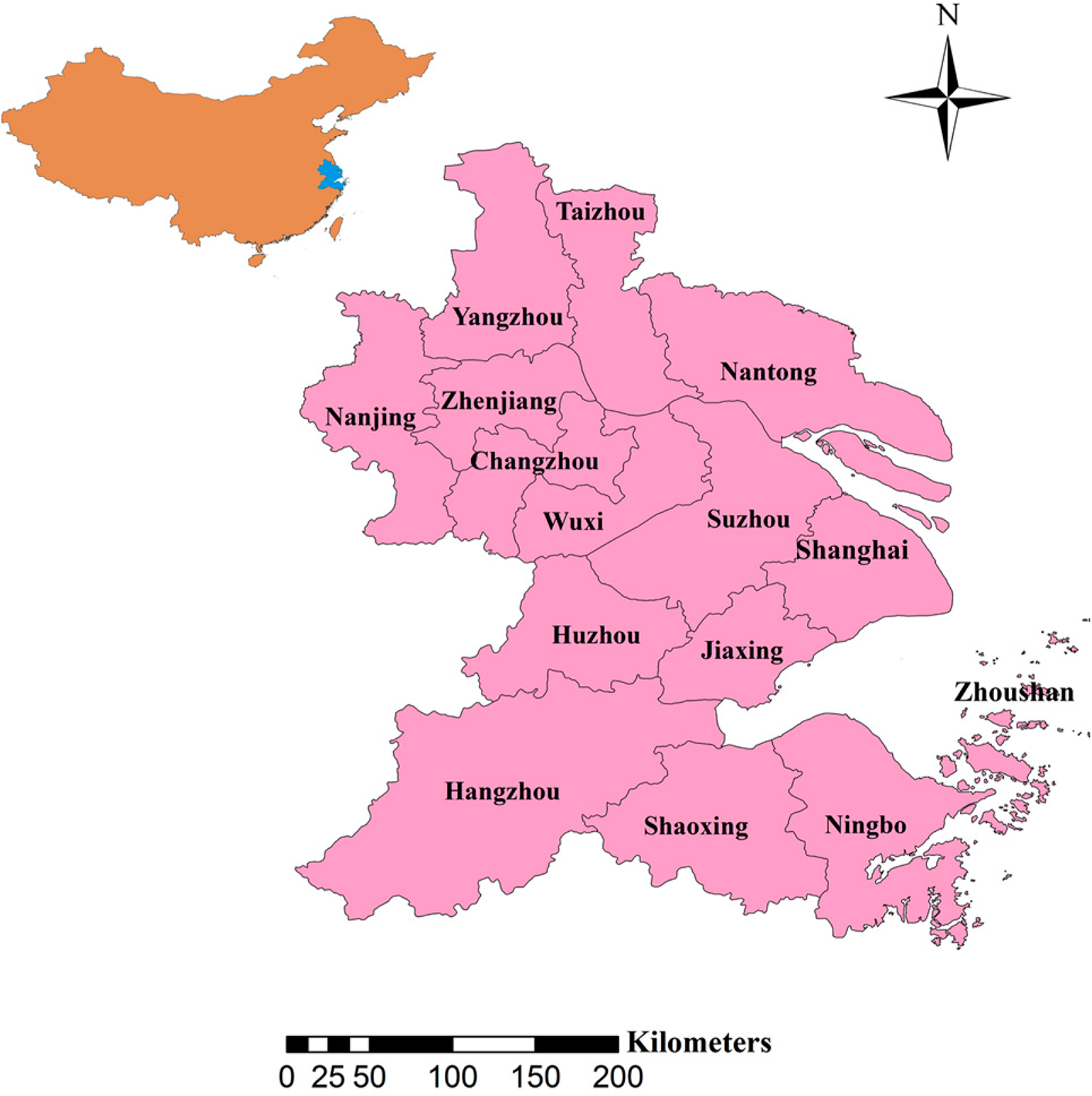
The Yangtze River Delta (YRD), with an area of approximately 118,000 km2, was selected as the study site. YRD is located in the lower reaches of the Yangtze River, covering the triangle-shaped territory of Shanghai, southern Jiangsu province and northern Zhejiang province in Eastern China. Figure 1 shows its geographic location and administrative divisions at the prefecture level (except for Shanghai, which is an administratively provincial unit). Flat land covered with a dense network of rivers accounts for the majority of YRD, while the remainder is hilly or mountainous. As one of China’s most densely populated regions, the YRD is growing into an influential world-class metropolitan area and playing an important role in China’s social development [41]. Accompanying the rapid economic development is the dramatic ISA growth, providing an ideal experimental opportunity for evaluating the utility of the developed method at the regional scale.
2.2. Data Collections
Multiple remotely sensed data sets were utilized in this study, and their major characteristics are summarized in Table 1. All collected data were spatially subset to the geographic extent of YRD and re-projected to a Lambert azimuthal equal area projection. The version 4 DMSP-OLS stable lights annual image composites for the years 2000–2009 were downloaded from the NOAA National Geophysical Data Center [42]. In order to minimize the data inconsistency, we only chose to use annual stable DMSP-OLS NTL derived from two satellites: F15 for the years 2000–2007 and F16 for the 2008–2009. Three MODIS products, including monthly NDVI (MOD13A3), land water mask (MOD44W) and yearly land cover data (MCD12Q1 version 5.1), were downloaded from the NASA Earth Observing System Data and Information System [43]. We also obtained the January–June, 2010, global ISA fraction map released by the NOAA National Geophysical Data Center [44], which was used as a mono-temporal reference dataset (assuming no ISA fraction change during January–June in 2010). The selection of this product was based on the following considerations. First, currently, the NOAA ISA fraction dataset is the only available dataset providing global percentage of imperviousness information. Second, its reliability was reported by several prior research works. Potere et al. [45] investigated the applicability of eight global urban maps in different regions of the world and indicated that the NOAA ISA fraction dataset could be the optimal choice for continuous value urban extent applications in Southeast and East Asia. More importantly, the 2010 NOAA ISA fraction map was improved from its 2000–2001 product by using reference data derived from high spatial resolution imagery in China with a Google Earth-based tool [46], providing a relatively reliable product for scientific applications. Finally, we compared the 2010 NOAA ISA product with the 2009 GlobCover land cover map (300-m spatial resolution) and found a compatible total ISA result in the YRD (5181.37 km2 using NOAA ISA fraction data and 4933.19 km2 using GlobCover data).
3. Method
Several key steps are included in our method, and the whole workflow is described in Figure 2. First, an inter-calibration procedure was applied for generating radiometric-compatible DMSP-OLS NTL time series and a water masking was used for removing pixels dominated by water body. Subsequently, we obtained the Vegetation Adjusted NTL Urban Index (VANUI) time series with the integrated use of the preprocessed DMSP-OLS NTL and MODIS NDVI dataset [23], which served as an independent variable of the spatially adaptive regression model. This model allows regression coefficients to vary at the per-pixel level by incorporating inverse distance weights to the least squares solution technique. In order to produce multi-temporal ISA fraction results using a mono-temporal reference dataset, temporally stable signatures were extracted and a random stratified sampling strategy was adopted for the generation of training and validation sets.
3.1. DMSP-OLS NTL Preprocessing
Due to the lack of in-flight calibration, the digital numbers among annual DMSP-OLS NTL images are not compatible. Here, we utilized a second order regression model proposed by Elvidge et al. [47] to generate inter-calibrated DMSP-OLS NTL time series. This model was empirically developed using some regions with little NTL change as the reference data. On this basis, other images can be adjusted to the same radiometric baseline. Detailed descriptions of the inter-calibration method and the regression equations can be found in [32,47]. The 250-m MODIS MOD44W product was degraded to 1-km spatial resolution, and pixels with a water fraction greater than 50% were filtered out to reduce the blooming effect along the coastline regions [26].
3.2. VANUI Time Series Generation
The Vegetation Adjusted NTL Urban Index (VANUI) was developed by Zhang et al. [23] to reduce the light saturation effect and enhance the intra-urban variance of DMSP-OLS NTL data. Although not specifically designed for ISA estimation, VANUI was found to be positively correlated with the percent of imperviousness [23,48]. In addition, it is straightforward and easy to implement and can be used as a feasible tool for long-term ISA fraction dynamic analysis.
VANUI was calculated with Equation (1):
3.3. Temporally Stable Signature Extraction
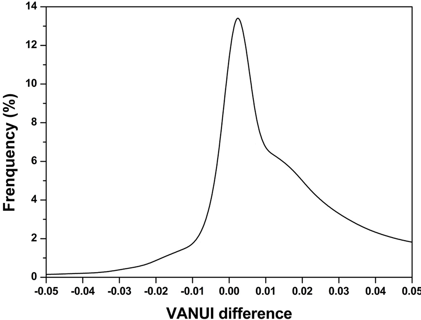
A key issue to reliably characterizing land cover dynamics using the classification technique is the derivation of a time-consistent training set [40,49]. Similarly, it is necessary to use temporally stable samples to construct a reliable ISA fraction-VANUI equation for each time series slice using a mono-temporal reference dataset. Gray and Song [40] developed an automatic adaptive signature generalization (AASG) approach for the selection of unchanged pixels between the image pair acquired on different dates. It should be noted that there is an implicit hypothesis in the AASG approach that the majority of image pixels are unchanged, resulting in a histogram distribution of the difference image with stable pixels located in an interval around the mean. In other words, the bias between the distribution mean value and the origin is solely caused by systemic uncertainties, such as the co-registration error. However, this assumption is probably invalid in this study. As shown in Figure 3, the histogram of the difference image between VANUI images acquired on different dates exhibits a skewed curve, indicating a biased mean value mainly introduced by the ISA increasing within the study area.
In this study, we extracted temporally stable samples using the following steps. First, a difference image was generated from the VANUI image pair acquired in the years 2000 and 2009, respectively. Second, a thresholding method was adopted for the selection of temporally stable pixel candidates [40]. Here, we assumed that systemic uncertainties were negligible, and therefore, unchanged pixels were located in the interval 0 ± c × ơ, where ơ represents the standard deviation of the difference image; c is a constant coefficient constraining the interval range, and an empirical value of 0.5 was used in this study. In general, the determination of c is a tradeoff between two constraints: it should minimize the number of temporally unstable pixels, while on the other hand, there should be adequate samples for model construction [40]. Third, we used the reference image to assign ISA fraction values to pixels identified as temporally stable candidates, and an erode filter with a 3 × 3 window size was then applied for reducing the impact of the co-registration error. Finally, a stratified sampling strategy was used, and a total number of 874 stable samples were selected for model training and validation, respectively, with a ratio of 1:1.
To evaluate the reliability of extracted temporally stable sample pixels, the 500-m MCD12Q1 land cover data for 2001 and 2009 were utilized to generate a reference land cover change data set. Both land cover images were geo-linked and divided into 2 × 2 pixel blocks (1 km2). For each block, it was considered to be temporally stable if all of its pixels’ land cover(s) remain unchanged; otherwise, it was temporally unstable. The extracted stable samples derived from the VANUI image pair were then assigned to these blocks, and quantitative assessment was implemented for the accuracy evaluation.
3.4. Spatially Adaptive Regression Model
As previously mentioned, there is an implicit hypothesis of constant coefficients in most regression-based models for ISA estimation. This assumption, however, could be sometimes violated. For example, Letu et al. [22] found that the ISA fraction and unsaturated DMSP-OLS NTL were linearly correlated, but regression coefficients are likely to vary in different cities. Based on Tobler’s first law of geography, all attribute values on a geographic surface are related to each other, but close values are more strongly related than distant ones [50]. Accordingly, it is reasonable to assume that spatially close training samples should play a more important role in the derivation of regression coefficients than those further apart.
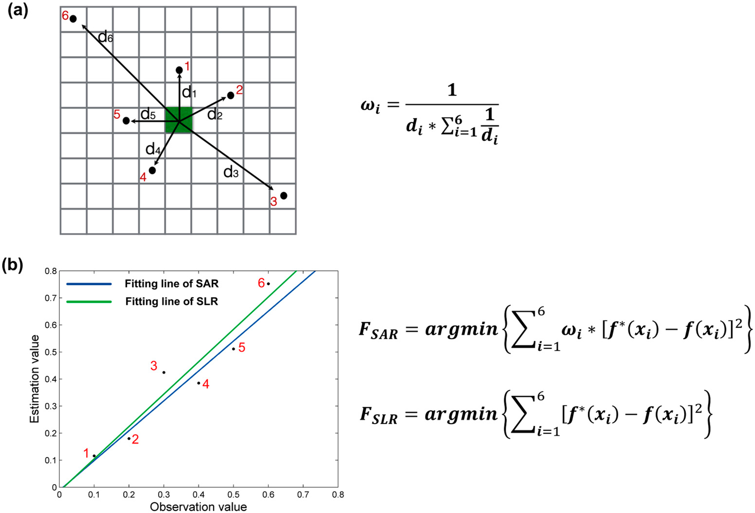
In this study, we proposed a straightforward method termed spatially adaptive regression (SAR) to accommodate the potential impact of spatial heterogeneity. Figure 4 illustrates the algorithm principle of SAR and its difference with the generalized least squares solution (LSS). As shown in Figure 4a, the green square represents the target pixel of which regression coefficients are unknown. Black points are training samples, and di indicates the Euclidean distance between training sample i and the target pixel. According to the generalized LSS approach, regression coefficients are obtained by minimizing the object function F, which is expressed by the sum of the squares of the residuals between observed results f(xi) and modeled results f*(xi). SAR, however, assumes each training sample is associated with a weight inversely proportional to the distance between the sample and the target pixel. Therefore, the object function is changed to minimize a weighted sum of squared residuals. Following this logic, sample Points 3 and 6 in Figure 4a are assigned with relatively small weights, due to their greater distance from the green square. As a result, the obtained fitting line of SAR will be different with the generalized LSS approach (see Figure 4b).
3.5. ISA Fraction Estimation Using the Spatially-Adaptive Regression Model
The linear model was selected to implement SAR because of its simplicity and reliability [23,48]. The reference ISA fraction was used as a dependent variable, and VANUI was used as an independent variable. Since generated regression coefficients vary across the image, we adopted the F-test and calculated the coefficient of determination (R2) for each validation sample to evaluate the model fitting performance. Here, the F-test was used to examine whether the regression model is significant, and R2 indicates the percentage of variation explained by the regression model.
3.6. Accuracy Assessment of ISA Fraction Estimation and Model Comparison
Three sub-pixel error metrics: root mean square error (RMSE), mean absolute error (MAE) and mean error (ME) were used to quantify the accuracy of estimated ISA fraction results. Here, RMSE and MAE measure the average levels of the absolute errors, while ME is an indicator quantifying systematic biases. Their formulae are described in Equations (2)–(4).
In order to further test the practicality of SAR, we also employed another two regression models, standard linear regression (SLR) and geographically-weighted regression (GWR), for comparison analysis. The standard linear model was developed using the same training dataset, but regression coefficients were derived from the generalized LSS approach. In contrast, GWR is a kernel-based regression technique to capture spatial variation [51]. In this study, GWR was implemented with the adaptive kernel type, and the extent of the kernel was determined by the Akaike information criterion (AICc). Readers can refer to Fotheringham et al. (2002) [52] for more details of the GWR principles.
4. Results
4.1. VANUI
A visual comparison with fine resolution images illustrates the superiority of VANUI for delineating urban ISA density. As shown in Figure 5, although both DMSP-OLS NTL and VANUI exhibit similar city outlines, we can clearly observe their differences. Saturated pixels were found in each city subset using DMSP-OLS NTL, indicating a potential loss of luminosity variability in urban cores. It was also found that this saturation effect became much more serious in large cities, such as Shanghai, with most of the areas associated with a red color. Therefore, it is inappropriate to directly use DMSP-OLS NTL for the estimation of the ISA fraction. On the contrary, VANUI utilizes NDVI as an additional scale factor to enhance intra-urban variability, which provides much finer details within urban cores. For example, it is obvious to find a hierarchical pattern of VANUI in Shanghai, with higher index values in the core urban region along the Huangpu River, while there are relatively low values around the city boundary, which is visually compatible with the spatial pattern of ISA density shown in the Landsat image. Similar results are also displayed in other two cities (Nanjing and Hangzhou), although the intra-urban variability is insignificant due to their relatively small city scales.
4.2. Accuracy Assessment of Temporally Stable Samples
Table 2 shows the accuracy assessment result of extracted temporally stable samples with the use of the MCD12Q1 product as the reference dataset. It is found that extracted stable samples provided overall satisfactory accuracy, indicated by the unchanged percentage of 88.22%. More importantly, there are various land cover change types for unstable samples, and only seven samples were identified as experiencing a natural to built-up transition, accounting for a percentage of 0.80%.
4.3. Fitting Performance of SAR
The fitting performance of SAR measured by the F-test and R2 was calculated annually and is displayed in Figure 6. It is found that all developed regression models are statistically significant at less than 0.0001 and provide average R2 greater than 0.55. In addition, we also observed no significant temporal increase or decrease trends, suggesting an acceptable robustness of the proposed model across different years.
4.4. Accuracy Assessment of ISA Fraction Estimation
A quantitative comparison of ISA fraction estimation using SAR, SLR and GWR was applied for the study site, and their results, measured by three error metrics, are displayed in Table 3. In general, all models slightly overestimated the ISA fraction, resulting in average ME values of 4.19%, 3.65% and 1.89%, respectively. Two spatially-specific models are found to provide lower average RMSE (16.18% for SAR, 16.38% for GWR) and MAE (12.41% for SAR, 13.17% for GWR) than SLR (17.95%, 15.30%, respectively), indicating enhanced model performances by incorporating spatial information. In particular, SAR outperforms the other two models measured by RMSE and MAE in all years, except for 2009, suggesting that it may offer an overall better estimation accuracy, although admittedly, its systematic bias is relatively large.
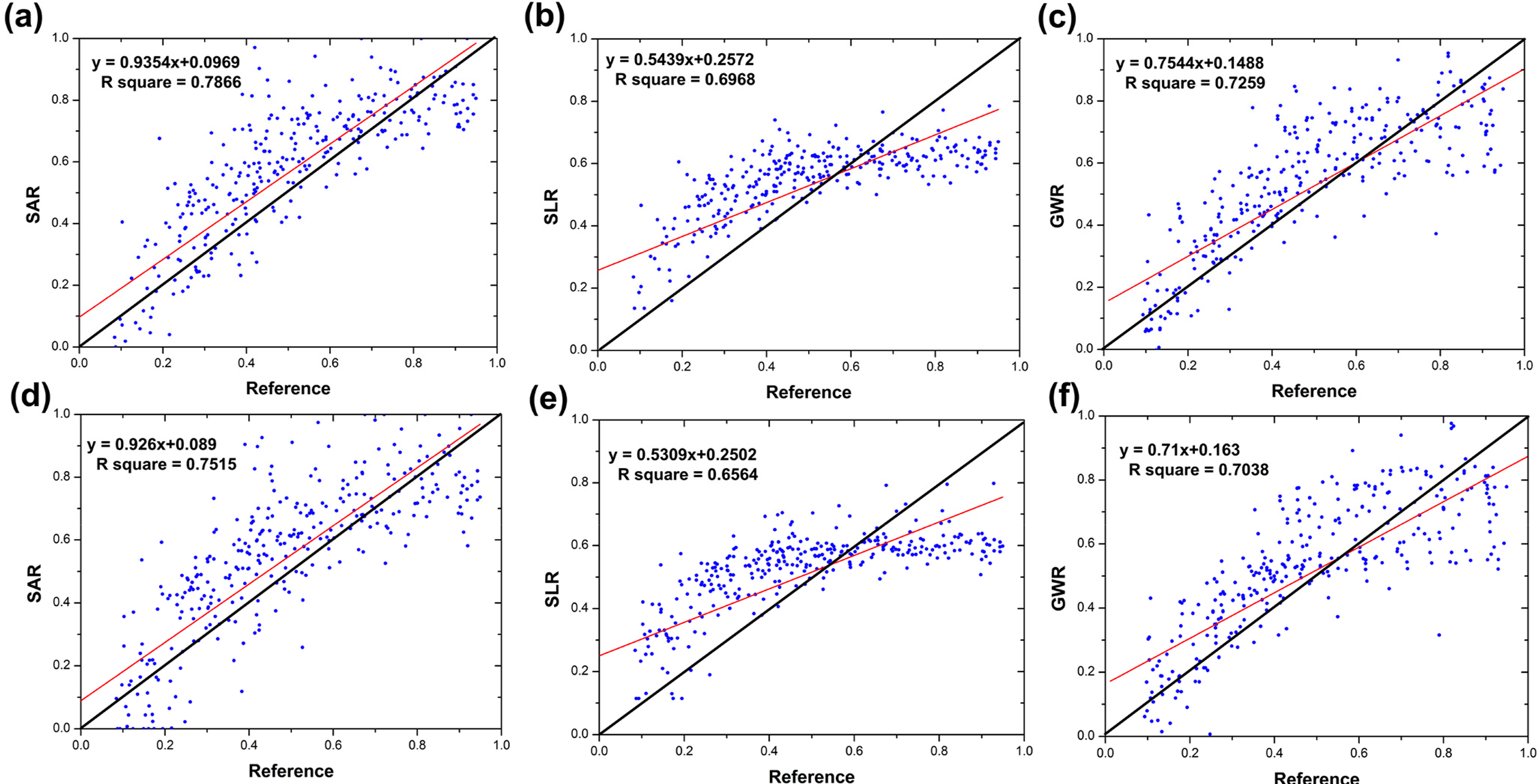
To further analyze model performances at different ISA fraction levels, we generated scatter plots between reference data and modeled results for two individual years (Figure 7). Generally speaking, both SAR and GWR display compatible distribution patterns and better agreements with reference data when compared to SLR, which tends to overestimate percentage of imperviousness at low ISA fraction levels, while underestimating it at high ISA fraction levels. Comparatively, SAR yields slightly better estimation consistency than GWR, with slopes closer to one and intersects closest to zero by comparing to the 1:1 line.
4.5. Spatial-Temporal Pattern of ISA in YRD
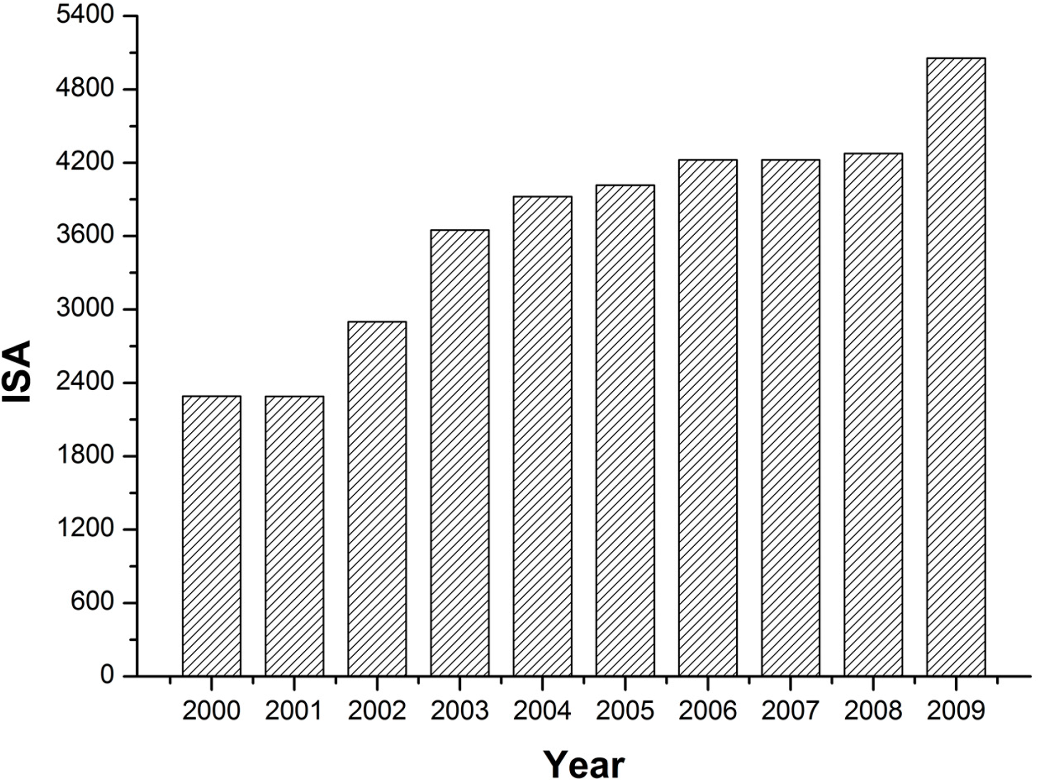
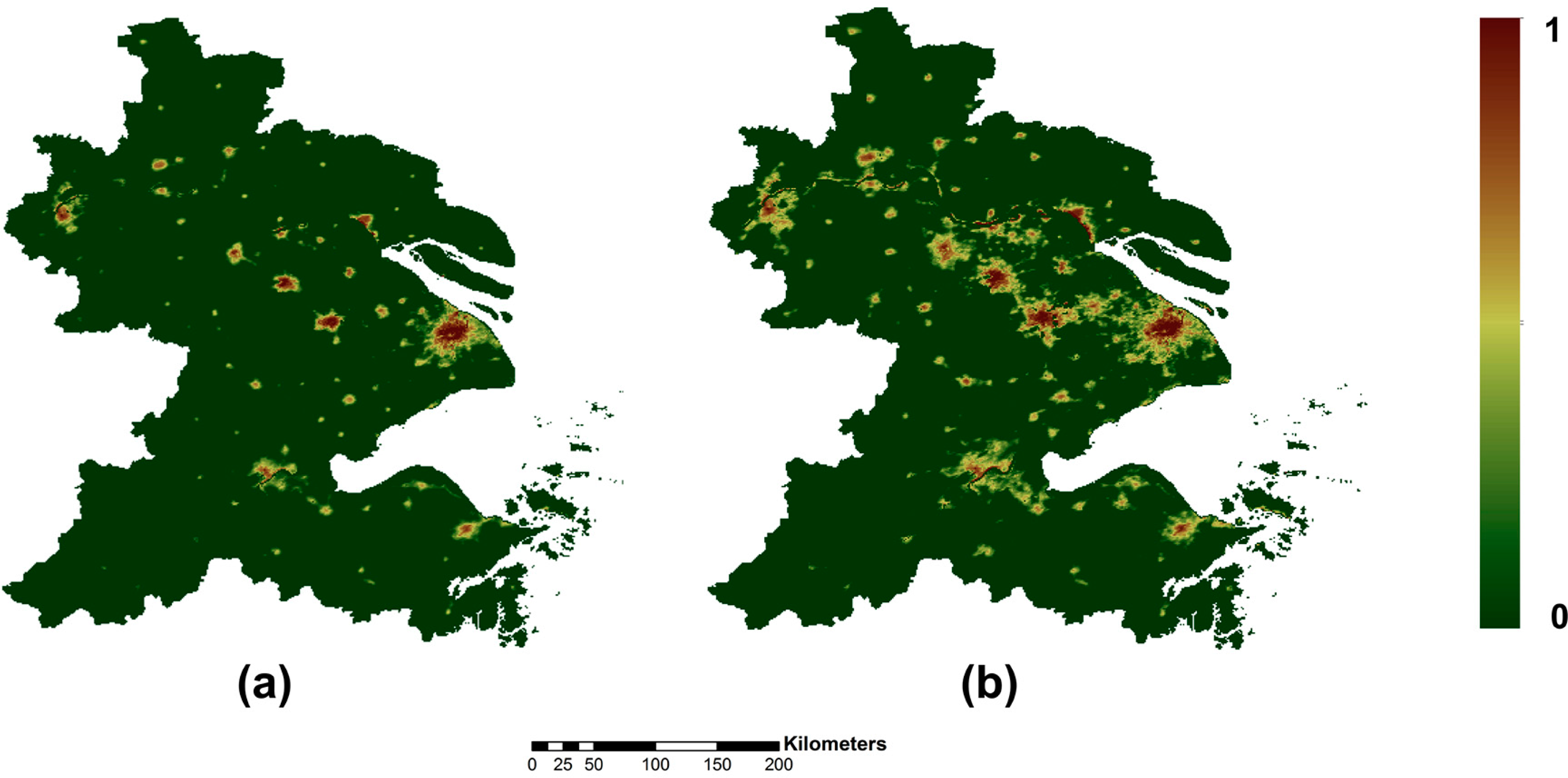
According to the multi-temporal ISA fraction estimation results with SAR, we found a rapid expansion of impervious surfaces in the Yangtze River Delta region during the decade 2000–2009, resulting in a total ISA increase of 2764.78 km2. It is also observed that the ISA growth rate varies substantially. As shown in Figure 8, two time periods, 2001–2004 and 2008–2009, account for the largest proportion of new ISA, while in other years’ increasing trends are relatively insignificant. Figure 9 displays the spatial dynamics of the ISA fraction in the YRD during 2000–2009. Through visual assessment, we can clearly find a diffusion-coalescence pattern of ISA expansion [53,54]. More specifically, in 2000, large-scale ISA was isolatedly observed in several well-developed cities, such as Shanghai, Hangzhou, Nanjing, etc., while these separated patches were then connected to each other in 2009 by filling gaps in between urban areas.
We further conducted a zonal analysis of ISA dynamics according to the administrative division of YRD, and the result is shown in Table 4. In particular, Shanghai exhibits the maximum ISA density, followed by Suzhou and Wuxi. Huzhou, Shaoxing and Zhoushan perform with the lowest average levels, with their ISA densities being less than 1% in 2000 and approaching 2% in 2009. In addition, substantial ISA expansion was found in each administrative region. Except for Shanghai and Ningbo, all other regions had more than 100% ISA growth rates during the decade. The largest growth rates are observed in Wuxi, Changzhou and Suzhou, with growth rates of 229.29%, 244.64% and 263.49%, respectively.
5. Discussion
5.1. Practical Considerations of VANUI
An important step for accurate ISA fraction estimation using regression models is the selection of independent variables. While initially developed to overcome the light saturation problem of DMSP-OLS NTL, VANUI exhibits the capacity of characterizing the intra-urban ISA fraction according to our investigation results. Compared to other indices using multiple sensor data sources, VANUI is more intuitive and easy to carry out, facilitating temporal dynamic analysis of the ISA fraction in a time and labor-efficient manner [48]. Although regarded as a powerful tool, VANUI should be used with several caveats. A primary uncertainty of VANUI may lie in the six-bit radiometric scale of DMSP-OLS. Due to the light saturation in urban cores, the utility of VANUI for the ISA fraction estimation may vary correspondingly. In addition, similar to other methods utilizing NTL data, VANUI is not capable of capturing ISA pixels with dark nighttime lights, such as low density residential areas and rural transportation pavements.
5.2. Comparison of SAR, LSR and GWR
This study also supported the utility of spatial information for ISA fraction estimation reported by previous studies. According to our investigation results, two spatially-specific models (SAR and GWR) exhibit substantial estimation improvements compared to SLR, which adopts a generalized LSS approach and assigns uniform weights to training samples. In theory, SAR and GWR are conceptually similar, because both of them assume varying model parameters at the per-pixel level and incorporate spatial information to enhance model performance. This similarity partially also explains the compatible estimation performances achieved by both models (see Table 3 and Figure 7).
Although theoretically related, there still exist distinct differences between SAR and GWR. The fundamental principle of GWR is kernel regression, through which model coefficients are determined by neighboring subsets of training samples, and therefore, the problem of spatial nonstationarity can be effectively addressed. However, careful attention should be given to the potential collinearity relationship due to the local nature of GWR [55,56]. As a result, it is usually recommended as a supplementary exploratory technique with global regression models for exploring the variability between variables within a geographical extent [52,56]. In contrast, SAR is developed using the entire training dataset, though neighboring samples are assigned with greater weights. In this sense, SAR may be regarded as a tradeoff between SLR and GWR. Furthermore, it is noteworthy that the relative performances of SAR and GWR can vary using different error metrics, highlighting more scientific efforts of the comprehensive comparison of these two models in the future.
5.3. Urban Dynamics in YRD
While it is generally accepted that there was a rapid urbanization trend in the YRD during past decades, actual quantitative results reported in the literature vary greatly. For example, Che et al. [57] provided a total urban extent of about 7000 km2 in 2007, while Hass and Ban [58] argued that the urban land in the YRD had achieved over 24,000 km2 in 2010. Although there is a time interval, it is nearly impossible to expect that the urban area tripled in three years. Actually, two primary uncertainties are associated with the disagreement indicated by previous studies. The first uncertainty comes from the lack of an unambiguous metric of urban expansion [30,31]. As previously mentioned, urban land and ISA are not theoretically equivalent. As a result, studies utilizing different metrics can lead to substantial result variations. More importantly, the selection of discrete pixel classification or sub-pixel fraction estimation can largely determine the final calculation result due to the different treatments to mixed pixels [54]. In particular, image pixels that are partially impervious may be classified as urbanized using the discrete classification, and therefore, a great uncertainty is expected. Kuang et al. [28] implemented a provincial ISA estimation in mainland China using sub-pixel fraction analysis, indicating a total urban ISA increase of 207.62 km2 in Shanghai during 2000–2008, which was similar to our result of 254.70 km2 during 2000–2009.
5.4. Limitations and Potential Improvements
In spite of the ability of estimating the multi-temporal ISA fraction at a large scale, the proposed method still has limitations. As an empirical approach, the performance of our model is largely dependent on the training data. In this study, we used the ISA fraction product from the NOAA National Geophysical Data Center, which obtained the global 1-km ISA fraction based on radiance calibrated DMSP-OLS NTL and Landscan population count [21]. It should be noted that the initial NOAA ISA fraction product in the year 2000–2001 was calibrated with the sole use of conterminous U.S. data, indicating a potential bias when the product is applied in other places. Although the 2010 product was improved by incorporating reference datasets from regions other than U.S., its accuracy is still to be further examined. This dilemma highlights the necessity of a more reliable global reference ISA fraction dataset, which can be generated from finer resolution land cover classification products. As previously discussed, the capability of VANUI would be greatly limited by the six-bit radiometric scale of DMSP-OLS. This problem can be solved by replacing DMSP-OLS NTL with the Visible Infrared Imaging Radiometer Suite (VIIRS) NTL acquired by the Suomi National Polar-orbiting Partnership (NPP) Satellite [23], which is currently available online [59]. With a wider radiometric range (14-bit) and finer spatial resolution (15 arcsec, approximately 500 m at the equator) [60,61], NPP-VIIRS NTL is expected to revolutionize scientific applications previously implemented by DMSP-OLS NTL and provides a further opportunity to improve our method.
6. Conclusions
In this study, a novel method was developed for estimating large-scale ISA fraction and analyzing its temporal dynamics with the integrated use of multiple sensor data sources. A regression model was employed to quantify the ISA fraction based on VANUI. This model allows regression coefficients to vary at the per-pixel level by incorporating spatial information in the generalized LSS approach and is capable of accommodating spatial heterogeneity in the training sample set. In order to acquire multi-temporal ISA fraction images with a mono-temporal reference dataset, we modified the AASG algorithm to extract temporally stable signatures for model training and validation. Our evaluation results indicated that the spatially adaptive regression model yielded substantial estimation improvements compared to the standard linear regression model and exhibited compatible performance with the geographically weighted regression model. According to our investigation, the Yangtze River Delta experienced a rapid ISA expansion during the decade 2000–2009, with a total increase of 2764.78 km2. The greatest ISA growth rates were found in boomtowns, including Wuxi, Changzhou and Suzhou, with their annual average growth rates being more than 20%. The proposed method is particularly valuable in large regions with a high speed of urban development, where traditional regression models suffer from spatial and temporal variance. Future improvements of the method may include the utilization of NPP VIIRS NTL for generating VANUI [23] and adopting a more reliable reference ISA fraction dataset.
Acknowledgments
The authors are grateful to four anonymous reviewers for their insightful comments and valuable suggestions. The authors also would like to thank NOAA’s National Geophysical Data Center (NGDC) and NASA’s Earth Science Data and Information System (ESDIS) Project for providing nighttime light and MODIS products. This work was supported by National Science and Technology Specific Projects (No. 2012YQ1601850 and No.2013BAH42F03), the National Natural Science Foundation of China (No. 61172174), the Program for New Century Excellent Talents in University (No. NCET-12-0426) and the Basic Research Program of Hubei Province (No. 2013CFA024).
Author Contributions
Zhenfeng Shao and Chong Liu conceived this research. Chong Liu performed experiments and wrote the manuscript. Zhenfeng Shao analyzed data and edited the manuscript.
Conflicts of Interest
The authors declare no conflict of interest.
References
- Grimm, N.B.; Faeth, S.H.; Golubiewski, N.E. Global change and the ecology of cities. Science 2008, 319, 756–760. [Google Scholar]
- Slonecker, E.T.; Jennings, D.; Garofalo, D. Remote sensing of impervious surface: A review. Remote Sens. Rev 2001, 20, 227–255. [Google Scholar]
- Arnold, C.L., Jr; Gibbons, C.J. Impervious surface coverage: The emergence of a key environmental indicator. J. Am. Plan. Assoc 1996, 62, 243–258. [Google Scholar]
- Schueler, T.R. The importance of imperviousness. Watershed Prot. Tech 1994, 1, 100–111. [Google Scholar]
- Schueler, T.R.; Fraley-McNeal, L.; Cappiella, K. Is impervious cover still important? Review of recent research. J. Hydrol. Eng 2009, 14, 309–315. [Google Scholar]
- Weng, Q. Remote sensing of impervious surfaces in the urban areas: Requirements, methods, and trends. Remote Sens. Environ 2012, 117, 34–49. [Google Scholar]
- Lee, H.L.; Bang, K.W. Characterization of urban stormwater runoff. Water Res 2000, 34, 1773–1780. [Google Scholar]
- Brun, S.E.; Band, L.E. Simulating runoff behavior in an urbanizing watershed. Comput. Environ. Urban Syst 2000, 24, 5–22. [Google Scholar]
- Paul, M.J.; Meyer, J.L. Streams in the urban landscape. Annu. Rev. Ecol. Syst 2001, 32, 333–365. [Google Scholar]
- Brabec, E.; Schulte, S.; Richards, P.L. Impervious surfaces and water quality: A review of current literature and its implications for watershed. J. Plan. Lit 2002, 16, 499–514. [Google Scholar]
- Lu, D.; Xu, X.; Tian, H.; Moran, E.; Zhao, M.; Running, S.W. The effects of urbanization on net primary productivity in Southeastern China. Environ. Manag 2010, 46, 404–410. [Google Scholar]
- Milesi, C.; Elvidge, C.D.; Nemanni, R.R.; Running, S.W. Assessing the impact of urban land development on net primary productivity in the Southeastern United States. Remote Sens. Environ 2003, 86, 401–410. [Google Scholar]
- Changnon, S.A. Inadvertent weather modification in urban areas: Lessons for global climate change. Bull. Am. Meteorol. Soc 1992, 73, 619–627. [Google Scholar]
- Mahmoud, A.H.A. Analysis of the microclimatic and human comfort conditions in an urban park in hot and arid regions. Build. Environ 2011, 46, 2641–2656. [Google Scholar]
- Moore, A.A.; Palmer, M.A. Invertebrate biodiversity in agricultural and urban headwater streams: Implications for conservation and management. Ecol. Appl 2005, 15, 1169–1177. [Google Scholar]
- Deng, C.; Wu, C. The use of single-date MODIS imagery for estimating large scale urban impervious surface fraction with spectral mixture analysis and machine learning techniques. ISPRS J. Photogramm. Remote Sens 2013, 86, 100–110. [Google Scholar]
- Lu, D.; Batistellab, M.; Morana, E.; Hetricka, S.; Alves, D.; Brondizioa, E. Fractional forest cover mapping in the Brazilian Amazon with a combination of MODIS and TM images. Int. J. Remote Sens 2011, 32, 7131–7149. [Google Scholar]
- Knight, J.; Voth, M. Mapping impervious cover using multi-temporal MODIS NDVI data. IEEE J. Sel. Topics Appl. Earth Obs 2011, 4, 303–309. [Google Scholar]
- Yang, F.; Matsushita, B.; Fukushima, T.; Yang, W. Temporal mixture analysis for estimating impervious surface area from multi-temporal MODIS NDVI data in Japan. ISPRS J. Photogramm. Remote Sens 2012, 72, 90–98. [Google Scholar]
- Li, W.; Wu, C. Phenology-based temporal mixture analysis for estimating large scale impervious surface distributions. Int. J. Remote Sens 2014, 35, 779–795. [Google Scholar]
- Elvidge, C.D.; Tuttle, B.T.; Sutton, P.C.; Baugh, K.E.; Howard, A.T.; Milesi, C.; Bhaduri, B.; Nemani, R. Global distribution and density of constructed impervious surfaces. Sensors 2007, 7, 1962–1979. [Google Scholar]
- Letu, H.; Hara, M.; Yagi, H.; Naoki, K.; Tana, G.; Nishio, F.; Shuhei, O. Estimating energy consumption from night-time DMPS/OLS imagery after correcting for saturation effects. Int. J. Remote Sens 2010, 31, 4443–4458. [Google Scholar]
- Zhang, Q.; Schaaf, C.; Seto, K.C. The Vegetation Adjusted NTL Urban Index: A new approach to reduce saturation and increase variation in nighttime luminosity. Remote Sens. Environ 2013, 129, 32–41. [Google Scholar]
- Henderson, M.; Yeh, E.T.; Gong, P.; Elvidge, C.; Baugh, K. Validation of urban boundaries derived from global night-time satellite imagery. Int. J. Remote Sens 2003, 24, 595–609. [Google Scholar]
- Cao, X.; Chen, J.; Imura, H.; Higashi, O. A SVM-based method to extract urban areas from DMSP-OLS and SPOT VGT data. Remote Sens. Environ 2009, 113, 2205–2209. [Google Scholar]
- Zhou, Y.; Smith, S.J.; Elvidge, C.D.; Zhao, K.; Thomson, A.; Imhoff, M. A cluster-based method to map urban area from DMSP/OLS nightlights. Remote Sens. Environ 2014, 147, 173–185. [Google Scholar]
- Lu, D.; Tian, H.; Zhou, G.; Ge, H. Regional mapping of human settlements in southeastern China with multisensor remotely sensed data. Remote Sens. Environ 2008, 112, 3668–3679. [Google Scholar]
- Kuang, W.; Liu, J.; Zhang, Z.; Liu, D.; Xiang, B. Spatiotemporal dynamics of impervious surface areas across China during the early 21st century. Chin. Sci. Bull 2013, 58, 1691–1701. [Google Scholar]
- Ridd, M.K. Exploring a V-I-S (vegetation-impervious surface-soil) model for urban ecosystem analysis through remote sensing—Comparative anatomy for cities. Int. J. Remote Sens 1995, 16, 2165–2185. [Google Scholar]
- Schneider, A.; Friedl, M.; Potere, D. A new map of global urban extent from MODIS data. Environ. Res. Lett 2009, 4. [Google Scholar] [CrossRef]
- Schneider, A.; Friedl, M.; Potere, D. Monitoring urban areas globally using MODIS 500 m data: New methods and datasets based on “urban ecoregions”. Remote Sens. Environ 2010, 114, 1733–1746. [Google Scholar]
- Elvidge, C.; Hsu, F.C.; Baugh, K.E.; Ghosh, T. Global Urban Monitoring and Assessment through Earth Observation, 1st ed; CRC Press: Boca Raton, FL, USA, 2014. [Google Scholar]
- Zhang, Q.; Seto, K.C. Mapping urbanization dynamics at regional and global scales using multi-temporal DMSP/OLS nighttime light data. Remote Sens. Environ 2011, 115, 2320–2329. [Google Scholar]
- Letu, H.; Hara, M.; Tana, G.; Nishio, F. A saturated light correction method for DMSP/OLS nighttime satellite imagery. IEEE Trans. Geosci. Remote Sens 2012, 50, 389–396. [Google Scholar]
- Ziskin, D.; Baugh, K.; Hsu, F.C.; Ghosh, T.; Elvidge, C. Methods used for the 2006 radiance lights. Pro. Asia-Pac. Adv. Netw 2010, 30, 131–142. [Google Scholar]
- Li, X.; Xu, H.; Chen, X.; Li, C.F. Potential of NPP-VIIRS nighttime light imagery for modeling the regional economy of China. Remote Sens 2013, 5, 3057–3081. [Google Scholar]
- Liu, C.; Shao, Z.; Chen, M.; Luo, H. MNDISI: A multi-source composition index for impervious surface area estimation at the individual city scale. Remote Sens. Lett 2013, 4, 803–812. [Google Scholar]
- Deng, C.; Wu, C. A spatially adaptive spectral mixture analysis for mapping subpixel urban impervious surface distribution. Remote Sens. Environ 2013, 133, 62–70. [Google Scholar]
- Shi, C.; Wang, L. Incorporating spatial information in spectral unmixing: A review. Remote Sens. Environ 2014, 149, 70–87. [Google Scholar]
- Gray, J.; Song, C. Consistent classification of image time series with automatic adaptive signature generalization. Remote Sens. Environ 2013, 134, 333–341. [Google Scholar]
- Gu, C.; Hua, L.; Zhang, X.; Wang, X.; Guo, J. Climate change and urbanization in the Yangtze River Delta. Habitat Int 2011, 35, 544–552. [Google Scholar]
- Version 4 DMSP-OLS Nighttime Lights Time Series. Available online: http://ngdc.noaa.gov/eog/dmsp/downloadV4composites.html (accessed on 06 May 2014).
- NASA Earth Observing System Data and Information System. Available online: https://earthdata.nasa.gov/ (accessed on 07 May 2014).
- Global Distribution and Density of Constructed Impervious Surfaces. Available online: http://ngdc.noaa.gov/eog/dmsp/download_global_isa.html (accessed on 07 May 2014).
- Potere, D.; Schneider, A.; Angel, S.; Civco, D.L. Mapping urban areas on a global scale: Which of the eight maps now available is more accurate? Int. J. Remote Sens 2009, 30, 6531–6558. [Google Scholar]
- Sutton, P.C.; Elvidge, C.D.; Bough, K.E.; Ziskin, D. Mapping the constructed surface area density for China. Proc. Asia-Pac. Adv. Netw 2011, 31, 69–78. [Google Scholar]
- Elvidge, C.D.; Ziskin, D.; Bough, K.E.; Tuttle, B.T.; Ghosh, T.; Pack, D.W.; Erwin, E.H.; Zhizhin, M. A fifteen year record of global natural gas flaring derived from satellite data. Energies 2009, 2, 595–622. [Google Scholar]
- Ma, Q.; He, C.; Wu, J.; Liu, Z.; Zhang, Q.; Sun, Z. Quantifying spatiotemporal patterns of urban impervious surfaces in China: An improved assessment using nighttime light data. Landsc. Urban Plan 2014, 130, 36–49. [Google Scholar]
- Fortier, J.; Rogan, J.; Woodcock, C.E.; Runfola, D.M. Utilizing temporally invariant calibration sites to classify multiple dates and types of satellite imagery. Photogramm. Eng. Remote Sens 2011, 77, 181–189. [Google Scholar]
- Tobler, W. A computer movie simulating urban growth in the Detroit region. Econ. Geogr 1970, 46, 234–240. [Google Scholar]
- Brunsdon, C.; Fotheringham, A.S.; Charlton, M.E. Geographically weighted regression: A method for exploring spatial nonstationarity. Geogr. Anal 1996, 28, 281–298. [Google Scholar]
- Fotheringham, S.; Brunsdon, C.; Charlton, M.E. Geographically Weighted Regression: The Analysis of Spatially Varying Relationships; Wiley: New York, NY, USA, 2002; p. 269. [Google Scholar]
- Dietzel, C.; Oguz, H.; Hemphill, J.J.; Clarke, K.C.; Gzaulis, N. Diffusion and coalescence of Houston Metropolitan Area: Evidence supporting a new urban theory. Environ. Plan. B Plan. Des 2005, 32, 231–246. [Google Scholar]
- Gao, F.; de Colstoun, E.B.; Ma, R.; Weng, Q.; Masek, J.G.; Chen, J.; Pan, Y.; Song, C. Mapping impervious surface expansion using medium resolution satellite image time series: A case study in the Yangtze River Delta, China. Int. J. Remote Sens 2012, 33, 7609–7628. [Google Scholar]
- Wheeler, D.; Tiefelsdorf, M. Multicollinearity and correlation among local regression coefficients in geographically weighted regression. J. Geogr. Syst 2005, 7, 161–187. [Google Scholar]
- Windle, M.J.S.; Rose, G.A.; Devillers, R.; Fortin, M.-J. Exploring spatial non stationarity of fisheries survey data using geographically weighted regression (GWR): An example from the Northwest Atlantic. ICES Mar. Sci 2010, 67, 145–154. [Google Scholar]
- Che, Q.; Duan, X.; Guo, Y.; Wang, L; Cao, Y. Urban spatial expansion process, pattern and mechanism in Yangtze River Delta. Acta Geogr. Sin 2011, 66, 446–456. [Google Scholar]
- Haas, J.; Ban, Y. Urban growth and environmental impacts in Jing-Jin-Ji, the Yangtze, River Delta and the Pearl River Delta. Int. J. Appl. Earth Obs 2014, 30, 42–55. [Google Scholar]
- VIIRS DNB Cloud Free Composites. Available online: http://ngdc.noaa.gov/eog/viirs/download_monthly.html (accessed on 10 May 2014).
- Elvidge, C.D.; Baugh, K.E.; Zhizhin, M.; Hsu, F.-C. Why VIIRS data are superior to DMSP for mapping nighttime lights. Proc. Asia-Pac. Adv. Netw 2013, 35. [Google Scholar] [CrossRef]
- Liao, L.B.; Weiss, S.; Mills, S.; Hauss, B. Suomi NPP VIIRS day-night band on-orbit performance. J. Geophys. Res 2013, 118, 12705–12718. [Google Scholar]


| Abbreviation | Data Description | Spatial Resolution | Time Coverage |
|---|---|---|---|
| NTL | DMSP-OLS nighttime lights time series version 4 a | 1 km | 2000–2009 |
| MOD13A3 | MODIS monthly NDVI | 1 km | 2000–2009 |
| MOD44W | Land Water Mask | 250 m | NA |
| MCD12Q1 | Land cover product (IGBP classification scheme) | 500 m | 2001, 2009 |
| NOAA ISA | Global Impervious Surface Area | 1 km | January–June 2010 |
aSatellite F15 was used for the years 2000–2007, and satellite F16 was used for the years 2008–2009.
| Land Cover Change Type | Number of Samples | Percentage (%) |
|---|---|---|
| Unchanged | 771 | 88.22 |
| Crop to natural vegetation | 43 | 4.92 |
| Crop/natural vegetation to built-up | 7 | 0.80 |
| Others | 53 | 6.06 |
| 2000 | 2001 | 2002 | 2003 | 2004 | 2005 | 2006 | 2007 | 2008 | 2009 | Mean | ||
|---|---|---|---|---|---|---|---|---|---|---|---|---|
| SAR | RMSE | 15.09 | 14.66 | 15.42 | 16.37 | 17.08 | 16.98 | 15.95 | 17.15 | 16.97 | 16.15 | 16.18 |
| MAE | 11.44 | 11.33 | 11.76 | 12.42 | 13.1 | 13.06 | 12.28 | 13.28 | 13.17 | 12.24 | 12.41 | |
| ME | 3.89 | 3.49 | 3.67 | 4.11 | 5.00 | 4.68 | 4.31 | 4.43 | 4.69 | 3.63 | 4.19 | |
| SLR | RMSE | 16.64 | 16.96 | 17.5 | 18.16 | 18.34 | 18.57 | 18.09 | 18.61 | 18.85 | 17.8 | 17.95 |
| MAE | 14.15 | 14.48 | 14.9 | 15.48 | 15.65 | 15.86 | 15.45 | 15.81 | 16.07 | 15.13 | 15.30 | |
| ME | 3.65 | 3.44 | 3.25 | 3.54 | 3.89 | 3.91 | 3.72 | 3.65 | 3.65 | 3.84 | 3.65 | |
| GWR | RMSE | 15.19 | 15.18 | 16.06 | 16.54 | 17.33 | 17.18 | 16.65 | 16.80 | 16.99 | 15.91 | 16.38 |
| MAE | 11.85 | 12.16 | 12.88 | 13.27 | 14.11 | 14.06 | 13.44 | 13.59 | 13.69 | 12.60 | 13.17 | |
| ME | 2.07 | 1.99 | 1.78 | 1.96 | 2.60 | 2.32 | 1.75 | 1.89 | 1.51 | 1.07 | 1.89 | |
| Administrative Region | 2000 | 2009 | Dynamic Change | ||||
|---|---|---|---|---|---|---|---|
| Total ISA (km2) | ISA Density (%) | Total ISA (km2) | ISA Density (%) | Total ISA (km2) | ISA Density (%) | Growth Rate (%) | |
| Shanghai | 780.31 | 12.24 | 1,035.01 | 16.20 | 254.70 | 3.96 | 32.64 |
| Nanjing | 192.65 | 2.64 | 396.14 | 5.83 | 203.49 | 3.19 | 105.63 |
| Wuxi | 157.93 | 3.39 | 520.04 | 10.93 | 362.11 | 7.54 | 229.29 |
| Changzhou | 91.24 | 1.87 | 314.44 | 7.04 | 223.20 | 5.17 | 244.63 |
| Taizhou | 65.12 | 1.00 | 157.58 | 2.63 | 92.46 | 1.63 | 141.98 |
| Suzhou | 240.03 | 2.95 | 872.49 | 10.07 | 632.46 | 7.12 | 263.49 |
| Nantong | 101.54 | 1.12 | 253.87 | 2.87 | 152.33 | 1.75 | 150.02 |
| Yangzhou | 83.24 | 1.05 | 213.71 | 3.11 | 130.47 | 2.06 | 156.74 |
| Zhenjiang | 53.76 | 1.21 | 129.36 | 3.28 | 75.60 | 2.07 | 140.63 |
| Hangzhou | 192.10 | 1.22 | 430.10 | 2.54 | 238.00 | 1.32 | 123.89 |
| Ningbo | 174.49 | 2.13 | 327.49 | 3.78 | 153.00 | 1.65 | 87.68 |
| Jiaxing | 48.00 | 1.28 | 141.59 | 3.52 | 93.59 | 2.24 | 194.98 |
| Huzhou | 36.89 | 0.58 | 81.31 | 1.38 | 44.42 | 0.80 | 120.41 |
| Shaoxing | 64.12 | 0.80 | 161.24 | 2.02 | 97.12 | 1.22 | 151.47 |
| Zhoushan | 9.47 | 0.76 | 21.27 | 1.74 | 11.80 | 0.98 | 124.60 |
© 2014 by the authors; licensee MDPI, Basel, Switzerland This article is an open access article distributed under the terms and conditions of the Creative Commons Attribution license (http://creativecommons.org/licenses/by/4.0/).
Share and Cite
Shao, Z.; Liu, C. The Integrated Use of DMSP-OLS Nighttime Light and MODIS Data for Monitoring Large-Scale Impervious Surface Dynamics: A Case Study in the Yangtze River Delta. Remote Sens. 2014, 6, 9359-9378. https://doi.org/10.3390/rs6109359
Shao Z, Liu C. The Integrated Use of DMSP-OLS Nighttime Light and MODIS Data for Monitoring Large-Scale Impervious Surface Dynamics: A Case Study in the Yangtze River Delta. Remote Sensing. 2014; 6(10):9359-9378. https://doi.org/10.3390/rs6109359
Chicago/Turabian StyleShao, Zhenfeng, and Chong Liu. 2014. "The Integrated Use of DMSP-OLS Nighttime Light and MODIS Data for Monitoring Large-Scale Impervious Surface Dynamics: A Case Study in the Yangtze River Delta" Remote Sensing 6, no. 10: 9359-9378. https://doi.org/10.3390/rs6109359