Study of the Penetration Bias of ENVISAT Altimeter Observations over Antarctica in Comparison to ICESat Observations

Abstract
: The aim of this article is to characterize the penetration bias of the ENVIronmental SATellite (ENVISAT) radar altimeter over the Antarctic ice sheet through comparison with the more accurate measurements of the Ice, Cloud and land Elevation Satellite (ICESat) altimeter at crossover points. We studied the difference between ENVISAT and ICESat fluctuations over six years. We observed the same patterns between the leading edge width and the elevation difference. Both parameters are linked, and the major bias is due to the lengthening of the leading edge width due to the radar penetration. We show that the elevation difference between both altimeters and the leading edge width are linearly well-linked with a 0.8 Pearson correlation coefficient, whereas the slope effect over the coasts is difficult to analyze. When we analyze each crossover point temporal evolution locally, the linear correlation between the leading edge width and the elevation difference is between −0.6 and −1. Fitting a linear model between them, we find a reliability index greater than 0.7 for the Antarctic Plateau and Dronning Maud Land, which confirms that the penetration effect has a linear influence on the retrieved height. Moreover, we present results from SARAL/AltiKa (launched in February 2013) that confirm SARAL/AltiKa accuracy and the promising information it will provide.1. Introduction
Altimetry is one of the most powerful tools for detecting ice sheet surface changes, allowing us to estimate the contribution of ice sheets to sea-level rise. Since 1991, continental ice sheets, such as Greenland and Antarctica, have been observed and studied by altimetric satellites on the same orbit, including European Remote Sensing Satellite 1 and 2 (ERS1 and ERS2) [1]. The ENVIronmental SATellite (ENVISAT) was launched in 2002 by the European Space Agency (ESA) to link up with ERS1 and ERS2, covering latitudes between 81.5°S and 81.5°N with a 35-day repeat cycle, and it successfully supplied eight years of measurements until the end of its nominal orbit [2].
The biggest limitations to obtaining accurate results over ice sheets are the geophysical factors that affect radar altimeters measurements and the post-processing called retracking: the slope error due to the large footprint, the penetration into the snowpack and the surface roughness at different scales [2]. All of these effects are mixed together and produce a biased retrieved height. Several methods have been proposed to estimate elevation changes, and discrepancies exist between each bias found in the estimates [3–5]. These disagreements are a major limitation in the improvement of our understanding of ice sheet evolution and thus require further investigation. This paper focuses specifically on one of the effects: the penetration that occurs and its influence on the retrieved height with the post-processing taken into account. We first explain the principle of altimetry: the measurement and the post-processing, called retracking, and we describe the geophysical effects that alter the estimates to understand how to study the induced bias.
The return radar echo received by the altimeter is recorded through time, producing an altimetric waveform with three major parameters: the backscatter, the return power, and the leading edge width and trailing edge slope, which are estimated by the retracking algorithm [6,7]. Retracking consists of finding the point within the waveform where the height can be deduced. Over oceanic surfaces, the altimetric range is deduced from the mid-height of the leading edge width. Unfortunately, over ice sheets, this process is not always reliable because of various geophysical phenomena, the retracking algorithm estimates are biased. First, the approximately 15-km footprint does not efficiently sample the surface topography, which is less flat than ocean surfaces; slopes and centimeter/meter-scale (sastrugi) or kilometer-scale (megadunes) features affect the signal waveform [8]. Moreover, at the frequency used by the ENVISAT, ERS1 and ERS2 altimeters, i.e., 13.6 GHz, the radar wave penetrates into the snowpack [9]. Previous studies have shown a penetration depth of approximately ten meters [10,11]. The waveform signal over ice sheets is, thus, considered to be composed of a surface echo and a subsurface echo [12,13]. Specific retracking models exist in the scientific community and depend on the observed surface and the parameters chosen to create the algorithms. Some algorithms are based on the Brown model or use a threshold of the waveform peak amplitude or deduce the center of gravity [14–17]. Consequently, the surface elevation estimate depends on the retracking model chosen and the inaccuracy of the model is considered an error. This topic will be discussed later. In this paper, the Ice-2 retracking algorithm is used. It is based on the Brown model, fitting the altimetric waveform with an error function (erf) for the leading edge and an exponential decrease for the trailing edge slope and deduce the waveform integration, thus providing the parameter estimates [7]. Moreover, from these waveform parameters, we can extract geophysical information on the surface properties, helping to understand the whole waveform signal and the retrieved height as well. The backscatter coefficient in dB is influenced by the surface or subsurface echo (consequently providing information on the surface roughness and snowpack properties), and the leading edge width (considered to be the amplitude of the width) is sensitive to the differently scaled features of the surface and volume [2]. The trailing edge slope characterizes the slope and the volume/surface ratio [18].
One of the major problems of this remote sensing method is that these snow parameters described above fluctuate through time. Consequently, the bias in the retrieved elevation is not constant and it affects the trend estimate, which leads to errors of up to 5 cm per year in the elevation trend [11]. Moreover, the penetration prevents us from directly comparing two altimeters with different frequencies. For instance, the ENVISAT follow-up, the 35-day orbit altimeter Satellite with ARgos and ALtika (SARAL or “simple” in hindi) with its Altimeter in Ka-band (AltiKa) works in the Ka-band; thus, both the volume scattering and the penetration depths are different. However, we show in this paper that a comparison between the Ku- and Ka-bands provides information.
Generally, the surface elevation change bias is corrected via the backscatter change [19]. This error is considered linearly dependent on the backscatter; thus, this is corrected by fitting temporal elevation series with the backscatter series. In 2012, Rémy et al. showed that the error could be better corrected if other waveform parameters were used, specifically the leading edge width [12]. This paper investigates this result by using a different six-year data set of laser altimetry to characterize the penetration effect on the retracking algorithm and the retrieved height, effect we call the penetration bias. Most of the studies based on the estimation of surface elevation changes have managed solely to reduce the induced noise but have not been able to estimate the absolute errors. Because the laser altimeter aboard the Ice Cloud and land Elevation Satellite (ICESat) is free from the systematic errors associated with radar altimetry over ice sheets, we decided to compare both measurements to characterize the radar altimeter’s biased height. The goal of this paper is to understand and help correct the penetration bias by exploiting the entire temporal data set from ICESat and the initial results from SARAL/AltiKa.
2. Data and Methods
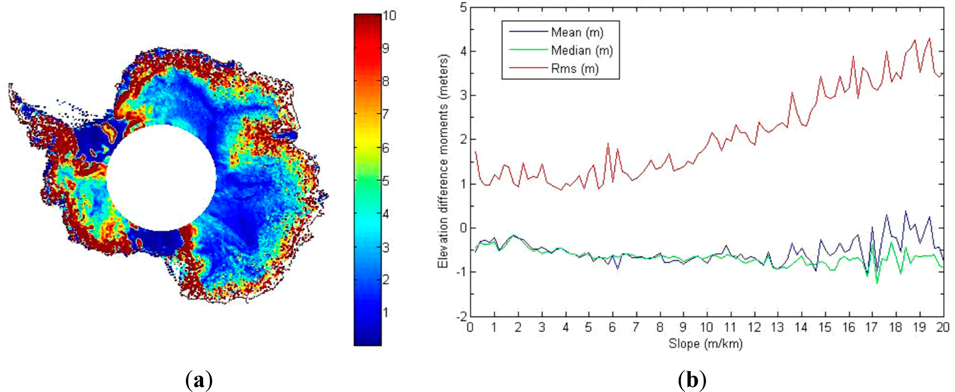
In 2003, ICESat, with the Geoscience Laser Altimeter System (GLAS) onboard, was launched by the National Aeronautics and Space Administration (NASA). GLAS is a laser altimeter (1064 and 532 nm wavelengths) that, with respect to Radar-Altimeter 2 (RA-2), more accurately retrieves elevation due to a narrower footprint (approximately 70 m instead of approximately 20 km for ENVISAT) and a non-penetration into the snowpack [3]. It also has a 40 Hz measurement frequency, which equates to a measurement every 170 m along the track, whereas the ENVISAT features a 20 Hz measurement frequency, or every 330 m. The saturation of the laser gain and the presence of clouds bias the elevation by preventing a global observation, but these biases are not as prevailing as the ones in radar altimetry and we are able to better characterize them [3]. To do so, we chose a crossover analysis between GLAS and RA-2. The ENVISAT and ICESat satellites observed the ice sheets at the same time, from 2002 to 2010 for ENVISAT and from 2003 to 2009 for ICESat. ENVISAT has a 35-day cycle, while ICESat has a 91-day cycle with 30- to 35-day campaigns. The elevation difference between ICESat and ENVISAT has been previously investigated, notably by Brenner et al. (2007), who found a 40 cm value with a 98 cm standard deviation (std) for flat surfaces and a 0.05 m value with a 25 m std for high slopes [3]. Brenner et al. found that the elevation difference is retracker-dependent [3]. We will discuss this later in the paper. The data we use are the height retrieved from ENVISAT with the Ice-2 algorithm, the height retrieved from ICESat with the Goddard Space Flight Center (GSFC-4) algorithm (the only algorithm used for ICESat data). The backscatter, the leading edge width and the trailing edge slope are all retrieved from ENVISAT with the Ice-2 algorithm. The first step in our processing is the correction of the slope effect for the six-year data from ENVISAT. Before performing the crossover analysis, we correct the RA-2 observations for the slope effect to compare more accurate radar altimetry elevations. Unlike oceanic surfaces (as mentioned in the Introduction part), ice sheets are sloped surfaces, over which the slope decreases from the coasts to the domes. Due to the slope and the 10- to 20-km footprint, the radar altimeter does not sample the surface well. The measured point is not necessarily located directly at the nadir, but is shifted in an upslope direction and is the closest point to the satellite. This shift induces a non-negligible bias that can add up to several meters to the retrieved height; this bias is known as slope-induced error [20]. The slope-induced error due to a large footprint can be corrected via three methods called relocation, slope correction (direct method), and the intermediate method [21,22]. The first method, used here, consists of finding the slope of the nadir and relocating the impact location to the estimated surface point closest to the altimeter antenna. To further analyze the slope-induced error, we map the mean slope at crossover points in m/km (Figure 1a) and the mean, std and median values of the elevation difference between ICESat and ENVISAT depending on the slope (Figure 1b). In Figure 1a, the slope is plotted across the entire Antarctic continent. The slope increases with increasing proximity to the coasts. Over the Plateau (Central Antarctica), the slope is mainly less than 2 m/km, but the slope is greater than 9 m/km (0.5°) along the coasts. Because ENVISAT has an antenna aperture of 1.35° (equivalent to a 18-km diameter footprint), the measurement is biased. Indeed, if the slope angle is higher than the mid-aperture, i.e., approximately 0.65°, the impact point of the altimeter will be on the edge of the footprint [23]. The altimeter impact is out of the gain pattern for ENVISAT; thus, the impact point might be closer and the slope correction greater than first thought, which explains the positivity of the elevation difference. We conclude that if the slope is greater than 9 m/km, the analysis cannot be as accurate as that of flat surfaces. In Figure 1b, we observe the different moments like the mean, and the std but also the median of the elevation difference in meters depending on the slope range. As evidence, we see that the greater is the slope; the greater is the elevation difference in absolute value. Until 9 m/km, the median and the mean are in good agreement and the std rather constant until 8m/km. The high std value between 0 and 1 m/km is due to the ice shelves. After 9 m/km we are out of the antenna gain, so no analysis can be done. The elevation difference is about −0.5 m. The std increases with the slope due to the residual slope error. The relation between the elevation difference and the slope is due to several effects. Note that it can be due to the slope error, because the Digital Elevation Models (DEMs) used to estimate the slope and relocate the position are not accurate enough or because we suffer from a limitation in the resolution [21,22]. Here, the slope is deduced from the across-track slope, which is derived from the whole ENVISAT cycles [23]. In addition, one cannot exclude the difference between both satellites footprints: the aperture of 1.35° explains a part of the measurement bias, which will be higher on the coasts indeed. As the error budget increases as the slope does, we do not take into account the highest slopes in our analysis. The data corrected from the slope error over flat surfaces is accurate enough to process it further so we deduce the crossover points between each measurement from both altimeters, the second step in our methodology.
Seventeen consecutive ICESat cycles were processed and compared to the measurements of the ENVISAT cycles (from cycle 20 to cycle 83, i.e., from September 2003 to November 2009) interpolated at the crossover intersection. The largest difference between each crossover point is 17 days, and the differences feature a uniform distribution and a std and a mean of eight days. We examined six years of observations, which has never been performed. The ICESat data are publicly available from the National Snow and Ice Data Center (NSIDC) website. We used the Level 2 product GLA12 (Antarctica and Greenland Surfaces). Several articles have been published on the biases involved with laser altimetry, especially the intercampaign bias associated with the Gaussian-Centroid (G-C) offset that potentially affects the elevation trend [24,25]. Because we do not compute any elevation trends in this paper (we study the quantitative differences between ENVISAT and ICESat elevations), it is not necessary to take this error into account.
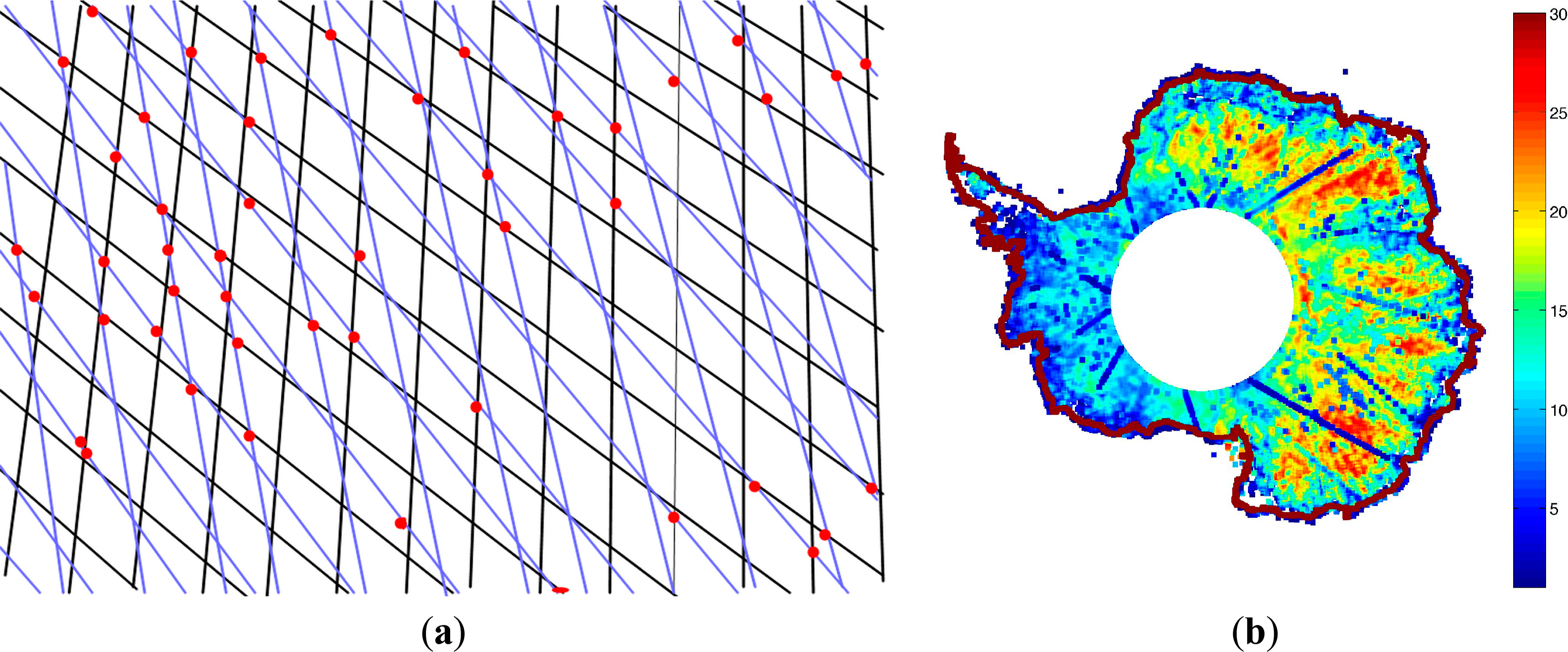
In Figure 2a,b, the crossover analysis is schematized (a) and the sampling plotted (b). In Figure 2a, we illustrate how the crossover method works, and we analyze the measurements provided by both altimeters at the same location. For the mean elevation difference, we analyzed all the crossover points spatially and temporally. For the temporal study, we chose to process locally, meaning we separated each crossover point and their evolution over six years and analyzed only the crossover points that were visited at least ten times a greater accuracy. By studying the evolution of a crossover point, we know that only both the surface undulations and the penetration influence the evolution measurement. In Figure 2b, we plot the number of measurements per each crossover point for the six-year duration. We confirm the sparser sampling over the coasts and West Antarctica, the reliability of the processing for the evolution is questionable. However, there is a denser sampling (more than ten times) over the Plateau. The third step in our methodology is attempting to fit a linear model between the elevation difference between ENVISAT and ICESat and the leading edge width. This relationship is as follows:
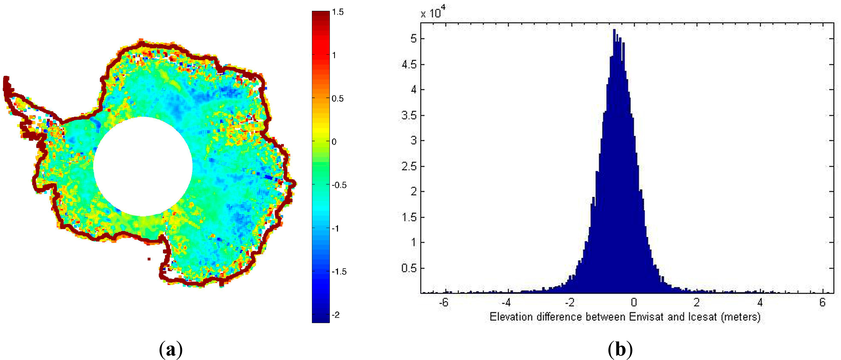
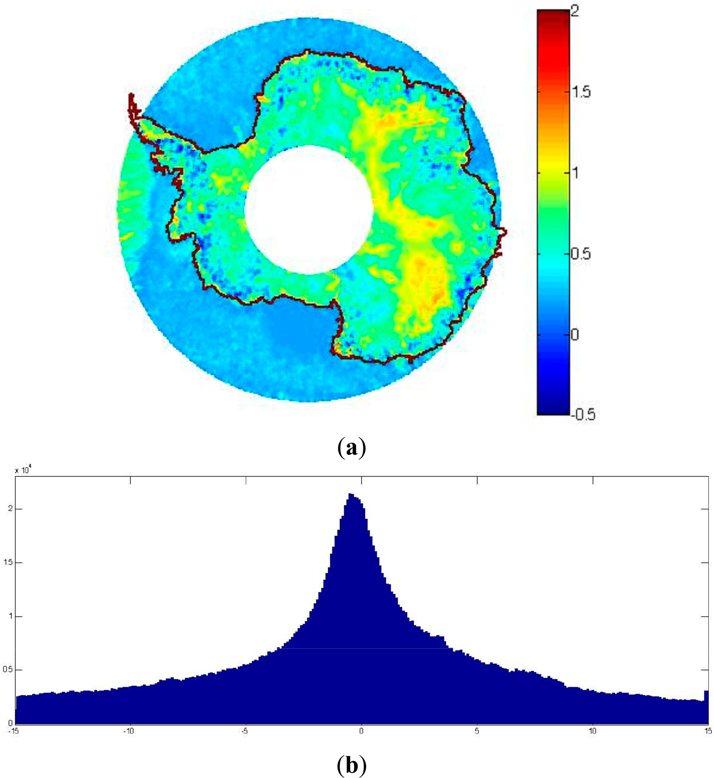
As a result after this three-part processing, we map the mean elevation differences corrected for the slope effect at the crossover points for the six-year duration that both ENVISAT and ICESat were in orbit in Figure 3a. Because of the penetration into the snowpack, the deduced radar elevation is lowered and the surface elevation value is lower than the laser one. Because ICESat is free from the penetration effect, the elevation difference is negative. This pattern is observed in the central part of Antarctica; the elevation difference is between −0.5 m and −1 m. However, the elevation is positive in the megadunes region. The slope is approximately 4 m/km in this region (in agreement with the Figure 1a) and the roughness is macro-scale; thus, the slope correction might be over-estimated, which explains the positive result. Figure 3b is the histogram showing the elevation difference between ICESat and ENVISAT when the slope is less than 9 m/km, a value chosen to keep measurements within the central part of Antarctica, according to Figure 1a,b, in which 9 m/km is the value at which the std increases. The mean and median are both approximately −0.53 m, and the std is 1.22 m. If we compare these results to the values of slopes greater than 9 m/km (not plotted), we find a mean of −0.61 m, a median of −0.63 m and a std of 2.77 m. The plot is coherent, the measurement error is lower, and there are fewer outliers in the data set when the slope is less than a given value, as the lower std value and nearly identical mean and median prove.
Consequently, due to the large uncertainties induced by the slope and the sparser sampling, we decided to remove the coasts and the Peninsula from the processing of the elevation differences between ICESat and ENVISAT and focus on a more reliable and valid data set.
If we do not take into account the residual slope error, the roughness at various scales, such as sastrugi or megadunes, and the penetration biases still affect the waveform [27]. In 2001, Arthern et al. showed the influence of surface undulations and microwave penetration using ERS1 and ERS2 measurements. Surface undulations are not the prevailing effect on the Plateau [7]. First, we focused our temporal analysis on areas that had been described by in situ measurements (for the geophysical information such as temperature or wind, surface characteristics) and satellites images located in the less steep areas of the Antarctic ice sheet. The surface roughness is considered to no effect on the retrieved elevation, as we will discuss later.
3. Results
3.1. Temporal Evolution across All of Antarctica
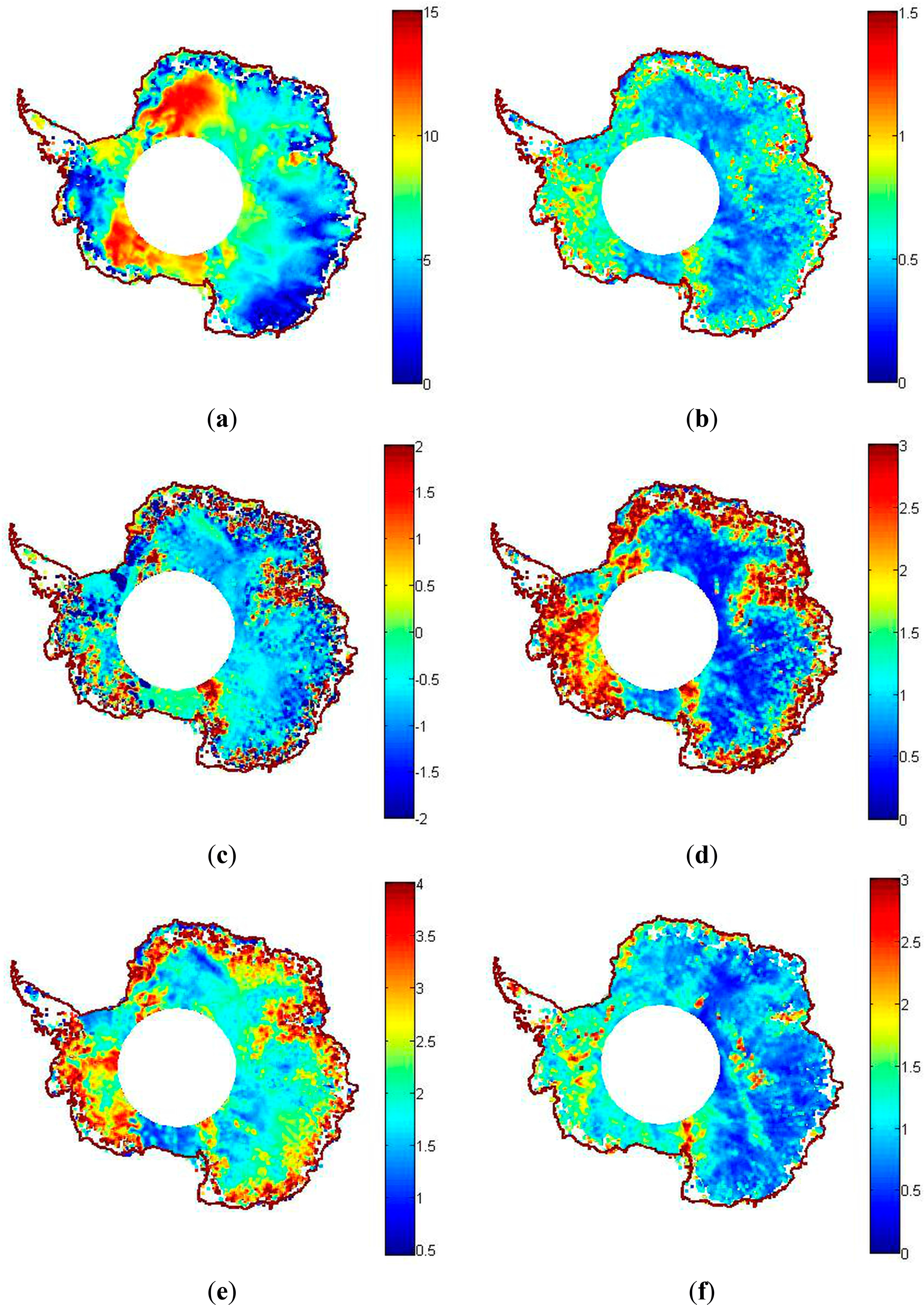
Up to 3,200,000 measurements, over six years, are available for the study of the variability in the evolution differences. Figure 4a–f contain the mean values over the entire period for the backscatter (a), the leading edge width (b) and the elevation difference (c) between both altimeters, as well as the std values (d–f). Note that we observed the evolution of the elevation difference, the backscatter coefficient from ENVISAT and the leading edge width from ENVISAT for the entire period, i.e., for each different ENVISAT cycle. We observed recurring patterns in the elevation difference every 10 ENVISAT cycles, occurring in February, March and April. The elevation difference decreases in the north of the Australian Antarctic Territory. There are also similar patterns between the mean values of the leading edge width and the elevation difference fluctuations (Figure 4b,c), especially in the East Antarctica Plateau and Dronning Maud Land. These values are negatively correlated in the non-mountainous areas and the coasts, which are very steeply sloped. For instance, this pattern is especially true for the northern part of Dronning Maud Land, the Ross Ice Shelf, and the southern part of the Plateau. It has been shown that the variations are not due to a change in the snowpack height but by a seasonal density change that influences the waveform parameters, such as the backscatter and the leading edge width [27].
Indeed, it seems that a higher leading edge width corresponds to a higher absolute value of the elevation difference, whereas the backscatter coefficient does not seem to have a clear pattern associated with the elevation difference (Figure 4a,c). The backscatter has a dB peak in the northwestern part of Dronning Maud Land, but it not as high as the elevation difference and the leading edge width. The backscatter coefficient definitely influences the retrieved height, but if we observe the patterns, its influence does not seem to be as strong, or at least not as explicit, as that of the leading edge width. The backscatter is influenced by the snowpack properties and the penetration into the snowpack [17]. This paper’s hypothesis investigates whether the leading edge is directly impacted by the penetration and studies the effect of the penetration bias on the retrieved height.
We suggest that the penetration depth fluctuations, and, thus, the biases, might be linearly linked with the elevation difference between ICESat and ENVISAT. If we examine the std values of the same variables (Figure 4d–f), the similarity between the leading edge width and the elevation difference is found once again. In Dronning Maud Land and the Plateau, the std values are low for both the height and the leading edge width, except for certain clear patterns in which they both increase. Along the coasts, the std increases for both the leading edge width and the elevation difference but not for the backscatter.
After a general overview, we focus on different locations in Dronning Maud Land, Mac. Roberston Land and the Plateau to validate our preliminary observations.
3.2. Focus on Four Specific Locations
To understand the retrieved height error, we attempt to link it with the waveform parameters to determine whether the penetration effect influences one or more waveform parameters, as has been previously suggested. The consensus up to now is that the variations in the backscatter are linked to the variations in the height [19]. The innovative idea here is to investigate whether the bias on the retrieved height is associated with the leading edge width (because the height is deduced from this parameter), and we did observe similar patterns through time. Moreover, Legrésy and Rémy showed that the leading edge is influenced by penetration and roughness at a micro-scale [17]. We selected data that were within 15 km of each location. We then analyzed the relationship between the leading edge width and the elevation difference. One such method is a scatter plot; by analyzing the shape, we can determine if the variables are linearly correlated or not. We also examined the values of the trailing edge and the backscatter between the leading edge width and the elevation difference in each scatter plot to determine whether we could separate the influence of surface undulations from the subsurface scattering [28–30]. The backscatter is influenced by the penetration via the snowpack properties but also by the surface properties. At the contrary, the leading edge width is solely affected by this effect. The trailing edge features positive values, indicating a volume echo. Because the trailing edge slope characterizes the volume/surface ratio, a higher ratio means a higher volume scattering.
3.2.1. Investigation of the Plateau Area
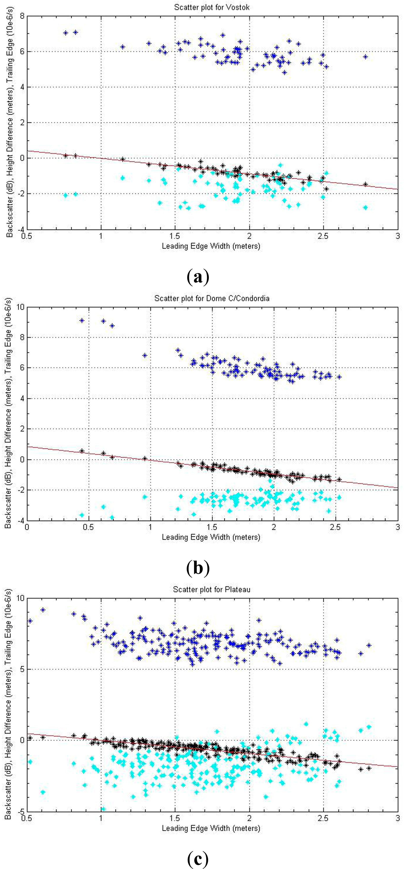
The Vostok area (106.837328°, −78.464422°) located in the Antarctic Plateau is characterized by a relatively flat surface. In Figure 5a, we show the scatter plot obtained for Vostok. One of the main observations is that correlation is clearly linear. The leading edge width ranges from 0.5 to 3 m, the difference ranges from −2 to 0.5 m, and these ranges are coherent with flat topography (the difference is mainly negative). Furthermore, when the elevation difference is close to zero, the leading edge value is close to one meter. This is, in general, a sign of a typical surface echo [6]. A larger absolute value of the elevation difference corresponds to a larger leading edge width, as was observed from the temporal evolution. A closer look at the values for the backscatter and the trailing edge reveals that when the elevation difference is close to zero, the backscatter is at its highest and the trailing edge slope is negative, which is indicative of a typical return echo from the surface [6]. The backscatter values are always above 5 dB. The trailing edge slope has values close to zero but negative, the surface is flat and the difference is low (−0.8 m), for sure there is a volume echo. The main observation is the dispersion of the different scatter plots. The leading edge width is the least dispersed scatter plot, which indicates a more intuitive linear relationship with the elevation difference, whereas the link is implicit and not necessarily linear for other parameters. By computing the Pearson correlation coefficient, we found a value of −0.9 between the elevation difference and the leading edge width in this particular location, statistically confirming the linear link. Furthermore, we fitted the linear relationship explained in the methodology part of Equation (1), and we obtained an alpha value of −0.87 and beta value estimate of 0.85. A linear relationship between the leading edge and the elevation difference is implied by these statistics. Note that we investigated the same type of relationship in this location between the backscatter and the elevation difference and found nothing significant. As a first empirical observation, this observation confirms that the fluctuation in the leading edge width and the penetration bias are linear in these two areas.
Dome C is also located on the Antarctic Plateau (123.35°, −75.1°). With no katabatic winds, the surface is less rough and can be considered flat. In Figure 5b, we show the scatter plot between the elevation difference and the leading edge width for Dome C. We find the same trends as for Vostok: the difference ranges from nearly 1 to −1.5 m and the leading edge ranges from 0.5 to 2.5 m. The Pearson correlation coefficient produces a value of −0.94, which is very high and proves that a fluctuation in the leading edge directly impacts the height estimate of flat surfaces. For the backscatter and trailing edge values, the backscatter is still above 5 dB, and the values almost never exceed −2 10−6·s−1 for the trailing edge, except when the difference is −0.91 m and the trailing edge is −1.4 10−6·s−1. This can be explained by a higher volume/surface ratio. The prevailing bias in this area is the penetration bias. Thus, we can link this effect linearly with the height bias, which has not been observed previously. The alpha and beta values are −0.9 and 0.84, respectively.
The Plateau station area is located in the central Plateau (40.56042°, −79.25082°). In Figure 5c, we clearly see a linearly shaped scatter plot. The leading edge width ranges from 0.5 to 2.8 m and the elevation difference from 0.2 to −2 m. The backscatter is always above 5 dB and decreases as the elevation difference increases, similar to the other areas. The trailing edge slope is high so there is volume scaterring. The Pearson coefficient between the leading edge width and the elevation difference is relatively high at −0.87, and the estimates for alpha and beta are −0.93 and 0.95, respectively, confirming the former observations.
3.2.2. Investigation of the Dronning Maud Land Area
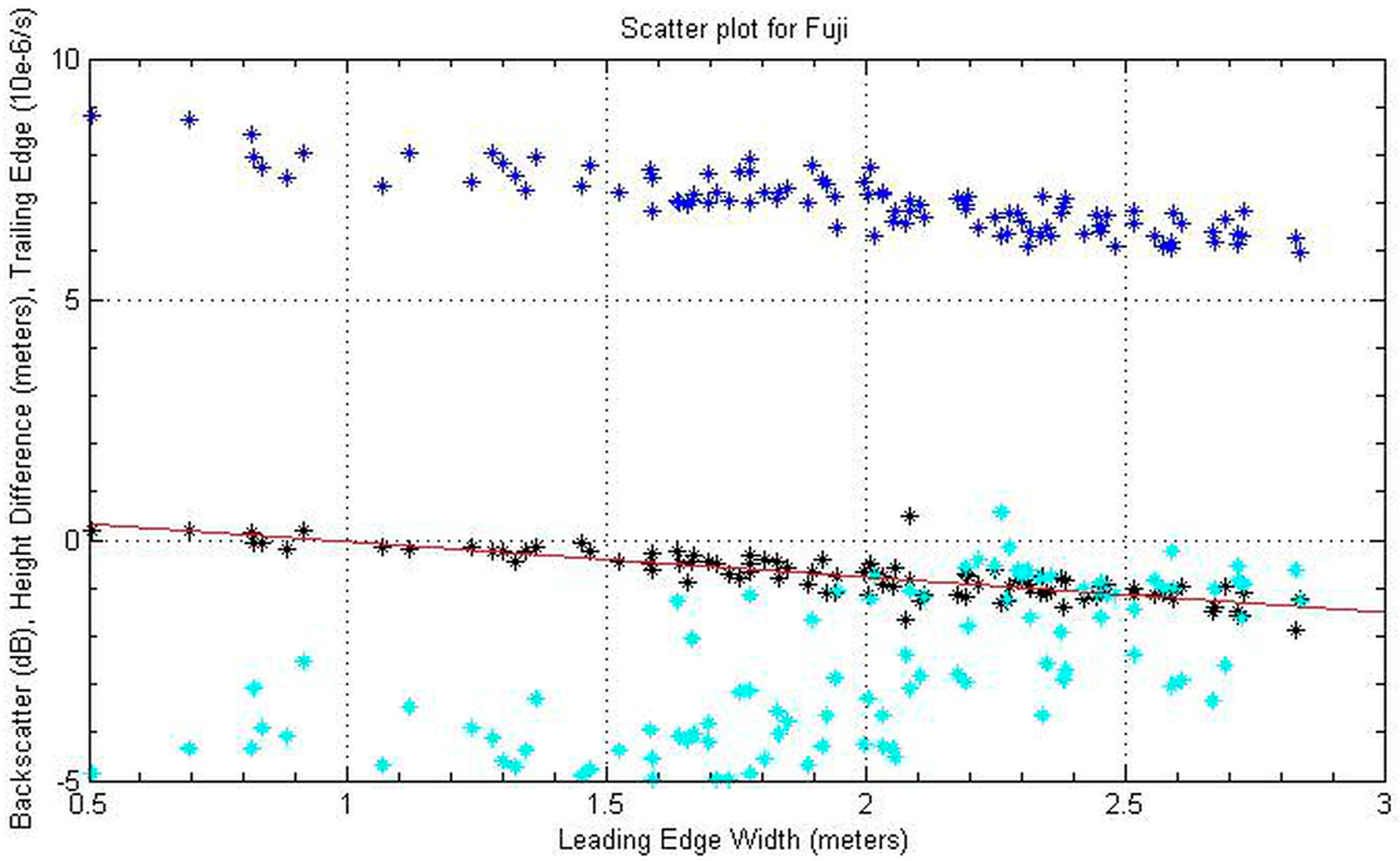
We next examined observations from near the Dome Fuji station (37.5°, −77.5°) in the Queen Maud Land (Northeastern Antarctica), which has been studied previously. In 2001, Arthern et al. showed through deconvolution that the surface undulations were not the prevailing effect in this area [7]. Legrésy and Rémy qualified Dronning Maud Land as a smooth surface [17].
The scatter plot in Figure 6 shows that the leading edge width ranges to 0.5 to 2.8 m and the elevation difference ranges from 0.3 m to −1.86 m. It is worth noting that the leading edge values are relatively stable in all the analyzed areas. Thus, the same effects seem to affect the leading edge width. The ratio between the volume and surface scattering can change, but the ratio features the same values here. This relationship is why we try to discriminate between the backscatter and the trailing edge. The backscatter values are greater than 6 dB, and the trailing edge is always negative when the leading edge is low and the backscatter is high. Thus, we have a pure surface echo [6]. However, once the leading edge width is greater than 1.5 m, the trailing edge features values near zero, and the penetration into the snowpack is clearly noticeable. Because the trailing edge has low absolute values as the elevation difference increases, we confirm the volume/surface ratio also has a high impact on the altimetric signal. Similar to the other flat areas, the scatter plot indicates a linear relationship between the leading edge width and the elevation difference. The Pearson correlation coefficient is −0.84 and the least-squares method produces values of −0.73 and a 0.69 for alpha and beta, respectively.
Table 1 summarizes the results of the study for all four areas. The values are concordant: the differences are approximately the same value as the backscatter and the leading edge width. The trailing edge slope is more variable. The trailing edge is a volume/surface ratio index; hence, we can interpret our values as a penetration depth modulated by the surface state. We conclude that there is a linear link between the leading edge width from ENVISAT and the elevation difference between ICESat and ENVISAT in the Antarctic Plateau and Queen Maud Land, where surface undulations are not the prevailing effects. Thus, we assume that it is the penetration effect, which includes a linear bias in the retrieved height: the penetration bias. The last column from Table 1 summarizes the std value of the differences once the model has been fitted. The results are satisfying because the std decreases.
We next examine if such a linear model can be fit to the entire Antarctic ice sheet instead of particular areas.
3.3. Fitting the Temporal Evolution to the Entirety of Antarctica
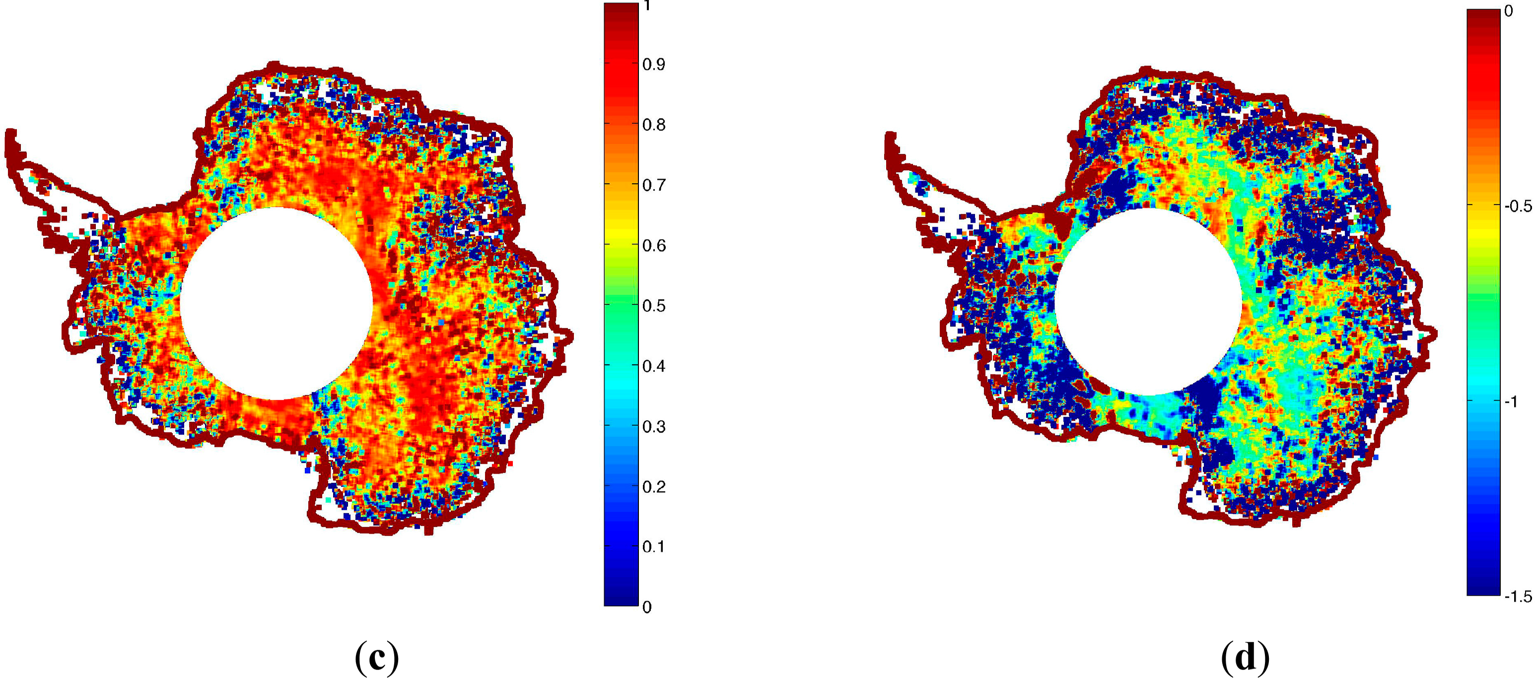
After observing a good linear fit between the leading edge and the elevation difference for various flat surfaces, we expand our study zone and process data from the entire Antarctic ice sheet. For computational reasons, we changed the reference to ENVISAT minus ICESat elevations instead of the former Equation (1), but this alteration changes only the sign of the estimated parameters. First, we plotted the linear correlation coefficient (as in the Pearson definition) between the leading edge width and the elevation difference between ENVISAT and ICESat in Figure 7a. There is a strong linear correlation between the elevation difference and the leading edge. On the Antarctic Plateau and Queen Maud Land, the absolute value is always higher than 0.6 for the Plateau and in very good agreement with the areas studied previously. Note that certain spots suggest a poor correlation, especially within the coasts as the first section described. In Figure 7b–d, we first see the SRC (b), then the estimates for alpha and beta using the linear regression explicited in the Equation (1). In places such as Vostok, Dome C and the Antarctic Plateau, the SRC coefficient is rather high, between 0.6 and the maximum value 1; thus, our model is reliable, and the linearity is not an incorrect hypothesis. However, the closer the observations are to the coasts, the lower the SRC becomes, decreasing to less than 0.4. Certain other effects alter the waveform signal and reduce the linearity between the leading edge and the penetration bias. We know that the penetration effect prevails on flat surfaces, whereas the slope effect and variously scaled roughness occur together, thus, making the retracking estimates more difficult. In Figure 7b, the values for alpha always have an amplitude higher than 0.6 in the central part. These values are in good agreement with the estimates made for Vostok and Dome C. Figure 7d shows the plot of the beta estimates, which have a wider range than the alpha values. However, for the Plateau, both parameters seem to be negatively proportional (the ratio between the alpha and beta parameters, figure not shown, is close to the unit over the Antarctica Plateau). This relationship is coherent with the findings of the temporal observations. The alpha and beta values, when separated, cannot explain the entire model. The intercept parameter (beta) is necessary because the leading edge width value cannot physically be zero if there is no difference between both altimeters. Furthermore, the beta parameter can be considered to be the mean value for the penetration depth, and alpha corrects for its variability by fluctuating along with the leading edge width. One way to check the model reliability is to analyze the residuals e(t) from Equation (1). The residuals have to be independent from the leading edge width and fit a Gaussian distribution, as the hypothesis of the model fitting suggests. We verified these factors by generating the scatter plot between the leading edge width and the residuals and confirmed the independence of these parameters. Moreover, the histogram of the residuals fits a Gaussian distribution. The linearity is satisfactory. The correction required to retrieve an accurate height can be considered to be a portion of the leading edge in meters. We study this hypothesis in the Discussion section.
4. SARAL/AltiKa, the First Preliminary Results
SARAL, with AltiKa aboard, is a joint mission between the French Space Agency (CNES) and the Indian Space Agency (ISRO) that was successfully launched in February 2013. It is the follow-up to ERS1, ERS2 and ENVISAT, operating in the same orbit [31]. SARAL has the same altitude and the same 35-day cycle as ENVISAT and its predecessors. The great difference resides in the use of a new frequency in the Ka-band: 35.75 GHz instead of the former 13.6 GHz in the Ku-band. The benefits are large. The footprint is smaller, meaning a smaller slope error and a less intense waveform distortion due to topography. However, the initial results show that SARAL/AltiKa has less reliable measurements over the coasts, and the retracking provides un-exploitable waveforms. Moreover, the Ka bandwidth is 480 MHz instead of 320 MHz; thus, the leading edge will be better sampled. In addition, we benefit from less penetration into the snowpack; theoretical calculations estimate less than one meter of penetration depth instead of 5 to 10 m in the Ku-band [31]. For the first time ever, AltiKa observes the surfaces at nadir in a simultaneously active/passive manner. The main drawback is a poor return signal due to the effects of clouds and rain, but the models predict a low data loss rate [32]. AltiKa provides continuity in the observations, and it has proven essential to understanding the ice sheets’ dynamics and evolution, improving the electromagnetic models, and discerning the interaction of microwaves with the snowpack [25].
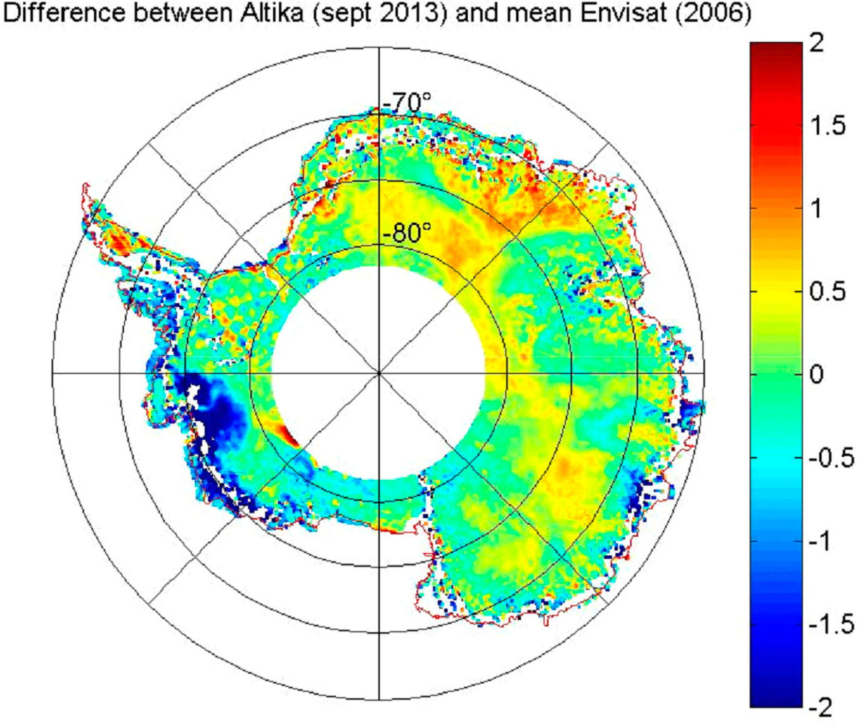
Figure 8 shows the difference between the mean profile from ENVISAT in 2006 and the along-track profile from SARAL in September 2013, when a maneuver to get SARAL on the same orbit as ENVISAT was performed. When Figures 3a and 8 are compared, we observe similar patterns. In the Dronning Maud Land, the elevation difference is the greatest in absolute value for both figures. Everywhere else, the elevations from SARAL/AltiKa are 0 to 0.5 m, higher than those of ENVISAT. This pattern confirms that the penetration depth in the Ka-band is lower than in the Ku-band [31]. However, because SARAL/AltiKa and ENVISAT have a different frequency, gain pattern, and crossover points in radar altimetry, the polarization of the antenna is a problem [33]. Moreover, they were not exactly in the same orbit for the first six months; thus, more observations need to be made. Note that occasionally the elevation differences are negative, which highlight the mass loss of the Amundsen Sea glaciers (West Antarctic Ice Sheet) [34]. Indeed, the elevation trend for the mass loss is 2 m per year, which leads to 6 m per year between the first cycle from SARAL and the last one from ENVISAT. Thus, the signal coming from the penetration is completely negligible.
5. Discussion
After having observed a dense data set between both altimeters and having studied the observations with signal processing methods, we can discuss our results.
The performed studies are retracker-dependent, as Brenner et al. demonstrated [3]. By using an algorithm based on a fitting function, the study showed that the GSFC-4 retracker is more efficient at calculating absolute elevations because it is less sensitive to the volume scattering than a threshold algorithm. It is known that a threshold-retracking algorithm is better suited to calculating elevation changes, but this is not the focus of this paper. In 1996, Davis studied different retracking algorithms, investigating the threshold level tuning for the threshold algorithms [11,35]. In Figure 9a, we plot the difference between two retracking algorithms for the Antarctic ice sheet: Ice-1 retracking uses the Offset Center of Gravity (OCOG) method, and Ice-2 is based on the Brown model. The difference is mainly positive, between 0.25 m to 1.25 m, suggesting that the Ice-2 retracking algorithm is more sensitive to volume scattering. However, the retracking algorithm Ice-1 uses a threshold value that is arbitrary and is not based on a physical model; thus, it can be more sensitive to surface properties [11]. In Figure 9b, the distribution of the elevation difference between the elevations derived from ICESat and the retracking algorithm Ice-1 is plotted for Antarctica, based on the 72nd cycle of ENVISAT. Interestingly, the elevation difference between both altimeters is not close to zero but is on the same magnitude as the difference between ICESat and Ice-2. This suggests that other error sources bias the Ice-1 retracking algorithm, and further investigation is needed. We suggest with this assumption that Ice-1 is less sensitive than Ice-2 to volume scattering, but note that every retracking algorithm has advantages and disadvantages. Furthermore, the Ice-2 retracking algorithm estimates the leading edge width, whereas the Ice-1 retracking algorithm uses a threshold to deduce the height [16,17]. The focus of this paper is to determine the effect of the penetration on the retrieved height, and the use of the leading edge width is essential for this purpose.
Finally, all of the studies we performed for this paper suggest a linear relationship between the penetration bias and the leading edge width. We confirmed that a simple linear model is suitable in the central East Antarctic Ice Sheet (EAIS). The spatial coherence between alpha and beta is due to the natural correlation between surface roughness, volume scattering, ice grain size or temperature that vary altogether with the altitude, explaining why a lot of parameters are geographically correlated. We calculated the corrected difference elevation in meters and plotted the portion of the leading edge width that we subtracted from the leading edge value estimated by the retracking algorithm in Figure 10. To calculate the percentage of the leading edge needed to retrieve the right surface elevation, it is assumed that the entire correction (right part of Equation (1)) is a portion of the leading edge, not taking into account the measurement errors (if not, the model cannot be simplified). By applying this empirical correction, the difference is approximately 0 m, except along the coasts (not shown because it is obvious). The std of the elevation difference is only 0.32 m instead of 2 m before fitting the linear model.
Former studies suggested a fixed position to compute the retracking algorithm. We estimated the mean value of the penetration bias in the retrieved height for the Ku-band over Antarctica to be approximately 1 m, which is in accordance with the first results from SARAL/AltiKa. This value is an empirical result represented by the beta value. The alpha value represents the fluctuations of the penetration depths that directly affect the lengthening of the leading edge width; we made corrections afterwards by shifting the position according to the location. Indeed, the location is important to understanding how the surface is observed by the altimeter due to the physical conditions. Note that the roughness is thought to have no effect on the altimetric signal. One argument in favor of a low surface roughness effect is that the linear relationship between the leading edge width and the elevation difference between ICEsat and ENVISAT is visible across the whole Antarctica Plateau, whereas the parameters for the surface roughness at the continental scale vary depending on the location. By comparing Figure 10 with the mean elevation difference between SARAL/AltiKa and ENVISAT (Figure 8), we observe that the portion of the leading edge width has higher values when the difference between SARAL/AltiKa is high. This suggests the same geophysical patterns but observed at a different frequency. We can keep up to 60% of the leading edge width and generally approximately 40%, in accordance with the elevation difference between ENVISAT and ICESat. Indeed, if we subtract 40% of the leading edge value, we keep 60% of the retracked value, which means we are close to the right retracking position. If we subtract more, we obtain a lower leading edge value, in accordance with the higher penetration depth. The greater the penetration effect is, the less we have to retrack in the leading edge width to avoid obtain a retrieved elevation below the height surface. Obviously, further studies need to be made to determine whether we can completely discriminate the different effects. One easily assumes that the effects of the slope, the penetration and the roughness are mixed together in the altimetric waveform; thus, the understanding of the retracked parameters is made more complex, especially along the coasts.
6. Conclusions
A six-year data set from ICESat and ENVISAT was processed to better understand a known bias that has been less studied and is still under investigation: the penetration bias on the retrieved height. The comparison between six years of observation from ICESat and ENVISAT was made because a study had already been conducted over a shorter period to assess the accuracy of laser altimetry [3]. This paper presents the longest period of comparison between laser altimetry and radar altimetry in the Ku-band. Similar patterns between the leading edge width and the elevation difference fluctuations are observed, suggesting a direct influence of the penetration effect over the leading edge width, i.e., the deduced height. To confirm this observation, a simple linear model between the leading edge width and the elevation difference between both altimeters was calculated and first performed for flat surfaces before applying it to the entirety of Antarctica, save for the more sloped areas, which are more complex to analyze and do not have a data set as dense as the flatter areas. The empirical penetration depth and its fluctuations of the ENVISAT altimeter were investigated to constrain the penetration bias. It is shown that it has a high variability combined with the mean penetration depth at each location, providing the penetration bias. The variability is approximately 0.6 m, and the mean penetration depth at each location is approximately 1 m. It is important to notice we constrained the penetration bias by observing the empirical penetration depth observed by the altimeters and not the theoretical penetration depth that can be higher but depending on the snowpack characteristics, its influence will not be as large as thought in the altimetric waveform. These observations are supported by the reliability of the model, which was studied with a model sensitivity analysis. Over the areas where the slope is less than 9 m/km and over ice shelves, the leading edge width has a strong influence on the retrieved height. Furthermore, this model is used to correct the penetration bias of the leading edge width, i.e., the retrieved height. Our observations show that the std of the corrected height is lower than before the correction. As the study is retracker-dependent, we focused on the algorithm we used and made an empirical observation of the leading edge tuning by calculating the portion of the leading edge width needed to retrack at the point corresponding to the first echo from the surface. The results are in agreement with previous studies on retracking algorithms; the leading edge needs to be lowered depending on the penetration effect and the lengthening can be as high as 80% in locations where the penetration depth effect is the strongest. Furthermore, the model implies a pure geometrical relation, through the lengthening the leading edge width. The issue previously was that when the elevation series are corrected with the backscatter series, it evolves with time. In this study, we just correct the leading edge geometrically, this relationship is stable with time.
Indeed, it is widely known that all the waveform parameters are influenced by the penetration of the radar wave into the snowpack (the penetration effect), but this study highlights the fact that the leading edge is influenced only by it. The other influences on the other waveform parameters are more difficult to model. Consequently, this study provides an estimate of the penetration bias that can be corrected solely for the leading edge width for the majority of the Plateau just by fitting a least-square model between the elevation difference and the leading edge width. For the coasts, the prevailing bias is not the penetration effect but the slope-induced error, which needs further studies to be ameliorated.
SARAL/AltiKa is the first altimetric mission operating on the Ka-band, which, by comparing with the Ku-band, allows us to better constrain the retracking algorithms inaccuracies and the physics of both frequencies. SARAL/AltiKa does not operate in the same frequency or even the same period, but it is the only way to compare former satellites on the same orbit. The first preliminary results provide a lower elevation difference between ENVISAT and SARAL/AltiKa, which tends to prove a lower penetration depth than in Ku-band, depth valuing approximately 0.3 m. SARAL/AltiKa is still under investigation, and as long as it is exploited, the studies will provide interesting results. Without any doubt, a comparison between ICESAT-2, due in 2017, and SARAL/AltiKa will be valuable to compare the Ka-band with laser altimetry, possibly to investigate the stability of the model according to the instrumental characteristics.
Acknowledgments
The author was granted CNES/CLS PhD funding. The altimetric data were provided by CTOH/Legos. The author is grateful to the four anonymous reviewers for their very relevant comments and the colleagues that helped with the English.
Author Contributions
Aurélie Michel wrote the article, implemented the methodology and the signal processing methods and made the data processing and analyzed them. Thomas Flament acquired the initial data and generated the crossover points. Frédérique Rémy did the article editing and helped with the analysis.
Conflicts of Interest
The authors declare no conflict of interest.
References
- Féménias, P.; Rémy, F.; Raizonville, P.; Minster, J.F. Analysis of satellite altimeter height measurements above ice sheets. J. Glaciol 1993, 133, 591–600. [Google Scholar]
- Rémy, F.; Parouty, S. Antarctic ice sheet and radar altimetry: A review. Remote Sens 2009, 1, 1212–1239. [Google Scholar]
- Brenner, A.C.; DiMarzio, J.R.; Zwally, H.J. Precision and accuracy of satellite radar and laser altimeter data over the continental ice sheets. IEEE Trans. Geosci. Remote Sens 2007, 45, 321–331. [Google Scholar]
- Cazenave, A.; Rémy, F. Sea level and climate: Measurements and causes of changes. Wiley Interdiscip. Rev. Clim. Chang 2011, 2, 647–662. [Google Scholar]
- Shepherd, A.; Ivins, E.R.; Geruo, A.; Barletta, V.R.; Bentley, M.J.; Bettadpur, S.; Briggs, K.H.; Bromwich, D.H.; Forsberg, R.; Galin, N.; et al. A reconciled estimate of ice-sheet mass balance. Science 2012, 338, 1183–1189. [Google Scholar]
- Hayne, G.S. Radar altimeter mean return waveforms from near-normal-incidence ocean surface scattering. IEEE Trans. Antennas. Propag 1980, AP-28, 687–692. [Google Scholar]
- Arthern, R.J.; Wingham, D.J.; Ridout, A.L. Controls on ERS altimeter measurements over ice sheets: Footprint-scale topography, backscatter fluctuations, and the dependence of microwave penetration depth on satellite orientation. J. Geophys. Res. Atmos 2001, 106, 33471–33484. [Google Scholar]
- Ridley, J.K.; Partington, K.C. A model of satellite radar altimeter return from ice sheets. Int. J. Remote Sens 1988, 9, 601–624. [Google Scholar]
- Legrésy, R.; Rémy, F. Using the temporal variability of satellite radar altimetric observations to map surface properties of the Antarctic ice sheet. Int. J. Glaciol 1998, 44, 197–206. [Google Scholar]
- Davis, H.C.; Poznyak, V.I. The depth of penetration in Antarctic firn at 10 Ghz. IEEE Trans. Geosci. Remote Sens 1993, 31, 1107–1111. [Google Scholar]
- Davis, H.C. A robust threshold retracking algorithm for measuring ice-sheet surface elevation change from satellite radar altimeters. IEEE Trans. Geosci. Remote Sens 1993, 35, 974–979. [Google Scholar]
- Rémy, F.; Flament, T.; Blarel, F.; Benveniste, J. Radar altimetry measurements over Antarctic ice sheet: A focus on antenna polarization and change in backscatter problems. Adv. Space Res 2012, 50, 998–1006. [Google Scholar]
- Brown, G.S. The average impulse response of a rough surface and its applications. IEEE Trans. Antennas Propag 1977, 25, 67–74. [Google Scholar]
- Laxon, S. Sea ice altimeter processing scheme at the EODC. Int. J 1994, 15, 915–924. [Google Scholar]
- Wingham, D.J.; Rapley, C.G.; Griffiths, H. New techniques in satellite altimeter tracking systems. In Proceedings of IGARSS’86 Symposium, Zürich, Switzerland, 8–11 September 1986; ESA Publications: Noordwijk, The Netherlands, 1986. [Google Scholar]
- Bamber, J.L. Ice sheet altimeter processing scheme. Int. J. Remote Sens 1994, 15, 925–938. [Google Scholar]
- Legrésy, B.; Papa, F.; Rémy, F.; Vinay, G.; van den Bosch, M.; Zanife, O.Z. ENVISAT radar altimeter measurements over continental surfaces and ice caps using the ICE-2 retracking algorithm. Remote Sens. Environ 2005, 95, 150–163. [Google Scholar]
- Legrésy, B.; Rémy, F. Surface characteristics of the Antarctic ice sheet and altimetric observations. J. Glaciol 1997, 43, 265–275. [Google Scholar]
- Zwally, J.H.; Giovinetto, M.B.; Li, J.; Cornejo, H.G.; Beckley, M.A.; Brenner, A.C.; Saba, J.L.; Yi, D.H. Mass changes of the Greenland and Antarctic ice sheets and shelves and contributions to sea-level rise: 1992–2002. J. Glaciol 2005, 51, 509–527. [Google Scholar]
- Brenner, A.C.; Bindschadler, R.A.; Thomas, R.H.; Zwally, H.J. Slope-induced errors in radar altimetry over continental ice sheets. J. Geophys. Res. Ocean. Atmos 1983, 88, 1617–1623. [Google Scholar]
- Hurkmans, R.T.W.L.; Bamber, J.L.; Griggs, J.A. Brief communication: Importance of slope-induced error correction in elevation change estimates from radar altimetry. Cryosphere 2012, 6, 447–451. [Google Scholar]
- Rémy, F.; Legrésy, B.; Bleuzen, S.; Vincent, P.; Minster, J.F. Dual-frequency TOPEX altimeter observation above Greenland. J. Electromagn. Waves Appl 1996, 10, 1505–1523. [Google Scholar]
- Rémy, F.; Flament, T.; Michel, A.; Verron, J. Ice sheet survey over Antarctica with satellite altimetry: ERS1/2, Envisat, Saral/AltiKa, the key importance of continuous observations along the same repeat orbit. Int. J. Remote Sens 2014, 35, 5497–5512. [Google Scholar]
- Borsa, A.A.; Moholdt, G.; Fricker, H.A.; Brunt, K.M. A range correction for ICESat and its potential impact on ice-sheet mass balance studies. Cryosphere 2014, 8, 345–357. [Google Scholar]
- Hofton, M.A.; Luthke, S.B.; Blair, J.B. Estimation of ICESat intercampaign elevation biases from comparison of lidar data in East Antarctica. Geophys. Res. Lett 2013, 40, 5698–5703. [Google Scholar]
- Jacques, J.; Lavergne, C.; Devictor, N. Sensitivity analysis in presence of model uncertainty and correlated inputs. Reliab. Eng. Syst. Saf 2006, 91, 1126–1134. [Google Scholar]
- Lacroix, P.; Dechambre, M.; Legrésy, B.; Blarel, F.; Rémy, F. On the use of the dual-frequency Envisat altimeter to determine snowpack properties of the Antarctic ice sheet. Remote Sens. Environ 2007, 112, 1712–1729. [Google Scholar]
- Champollion, N.; Picard, G.; Arnaud, L.; Lefebvre, E.; Fily, M. Hoar crystal development and disappearance at Dome C, Antarctica. Cryosphere 2013, 7, 1247–1262. [Google Scholar]
- Picard, G.; Royer, A.; Arnaud, L.; Fily, M. Influence of meter-scaled wind-formed features on the variability of the microwave brightness temperature around Dome C in Antarctica. Cryosphere 2013, 7, 3675–3716. [Google Scholar]
- Macelonni, G.; Brogioni, M.; Pampaloni, P.; Cagnati, A. Multifrequency microwave emission from the Dome C area on the East Antarctic Plateau temporal and spatial variability. IEEE Trans. Geosci. Remote Sens 2007, 45, 2029–2039. [Google Scholar]
- Vincent, P.; Steunou, N.; Caubet, E.; Phalippou, L.; Rey, L.; Thouvenot, E.; Verron, J. AltiKa: A Ka-band altimetry payload and system for operational altimetry during the GMES period. Sensors 2006, 6, 208–234. [Google Scholar]
- Tournadre, J.; Lambin-Artru, J.; Steunou, N. Cloud and rain effects on AltiKa/SARAL Ka-band radar Altimeter—Part I: Modeling and mean annual data availability. IEEE Trans. Geosci. Remote Sens 2009, 47, 1806–1817. [Google Scholar]
- Rémy, F.; Legrésy, B.; Benveniste, J. On the azimuthally anisotropy effects of polarization for altimetric measurements. IEEE Trans. Geosci. Remote Sens 2006, 44, 3289–3296. [Google Scholar]
- Flament, T.; Rémy, F. Dynamic thinning of Antarctic glaciers from along-track repeat radar altimetry. J. Glaciol 2012, 58, 830–840. [Google Scholar]
- Davis, C.H. A comparison of ice-sheet satellite altimeter retracking algorithms. IEEE Trans. Geosci. Remote Sens 1997, 34, 229–236. [Google Scholar]


| Location | Mean Leading Edge Width (m) | Mean Difference (m) | Std Leading Edge Width (m) | Std Difference (m) | Pearson Correlation Coefficient | Alpha Estimation | Beta Estimation |
|---|---|---|---|---|---|---|---|
| Plateau: 111 measurements | 1.71 | −0.66 | 0.45 | 0.48 | −0.87 | −0.93 | 0.95 |
| Vostok: 62 measurements | 1.92 | −0.81 | 0.38 | 0.36 | −0.90 | −0.87 | 0.85 |
| Dome C: 57 measurements | 1.79 | −0.77 | 0.40 | 0.38 | −0.94 | −0.90 | 0.84 |
| Dome Fuji: 78 measurements | 1.98 | −0.76 | 0.53 | 0.46 | −0.84 | −0.73 | 0.69 |
| Location | Mean Backscatter (dB) | Mean Trailing edge slope (10−6 s−1) | Std Backscatter (dB) | Std Trailing edge slope (10−6 s−1) | |||
| Plateau: 111 measurements | 6.82 | −1.74 | 0.72 | 1.08 | |||
| Vostok: 62 measurements | 5.87 | −1.66 | 0.51 | 0.62 | |||
| Dome C: 57 measurements | 6.01 | −2.63 | 0.74 | 0.40 | |||
| Dome Fuji: 78 measurements | 7.01 | −2.66 | 0.60 | 1.55 | |||
| Location | Std value for the elevation difference after the correction in meters | ||||||
| Plateau: 111 measurements | 0.23 | ||||||
| Vostok: 62 measurements | 0.31 | ||||||
| Dome C: 57 measurements | 0.32 | ||||||
| Dome Fuji: 78 measurements | 0.39 | ||||||
Note that the trailing edge values are more or less close to the nominal value, with no slope and no volume contribution, which is −3.2. The areas of our observations are relatively flat. The contribution comes from the volume echo.
© 2014 by the authors; licensee MDPI, Basel, Switzerland This article is an open access article distributed under the terms and conditions of the Creative Commons Attribution license (http://creativecommons.org/licenses/by/4.0/).
Share and Cite
Michel, A.; Flament, T.; Rémy, F. Study of the Penetration Bias of ENVISAT Altimeter Observations over Antarctica in Comparison to ICESat Observations. Remote Sens. 2014, 6, 9412-9434. https://doi.org/10.3390/rs6109412
Michel A, Flament T, Rémy F. Study of the Penetration Bias of ENVISAT Altimeter Observations over Antarctica in Comparison to ICESat Observations. Remote Sensing. 2014; 6(10):9412-9434. https://doi.org/10.3390/rs6109412
Chicago/Turabian StyleMichel, Aurélie, Thomas Flament, and Frédérique Rémy. 2014. "Study of the Penetration Bias of ENVISAT Altimeter Observations over Antarctica in Comparison to ICESat Observations" Remote Sensing 6, no. 10: 9412-9434. https://doi.org/10.3390/rs6109412