GPR Signal Characterization for Automated Landmine and UXO Detection Based on Machine Learning Techniques


Abstract
: Landmine clearance is an ongoing problem that currently affects millions of people around the world. This study evaluates the effectiveness of ground penetrating radar (GPR) in demining and unexploded ordnance detection using 2.3-GHz and 1-GHz high-frequency antennas. An automated detection tool based on machine learning techniques is also presented with the aim of automatically detecting underground explosive artifacts. A GPR survey was conducted on a designed scenario that included the most commonly buried items in historic battle fields, such as mines, projectiles and mortar grenades. The buried targets were identified using both frequencies, although the higher vertical resolution provided by the 2.3-GHz antenna allowed for better recognition of the reflection patterns. The targets were also detected automatically using machine learning techniques. Neural networks and logistic regression algorithms were shown to be able to discriminate between potential targets and clutter. The neural network had the most success, with accuracies ranging from 89% to 92% for the 1-GHz and 2.3-GHz antennas, respectively.1. Introduction
Mine detection is an ongoing and increasing problem that affects millions of people around the world, because of the enormous danger that mines represent to humans. Due to the long lifetime of these objects, the victims are often unrelated to the original conflict during which the mines were emplaced. Currently, millions of mines remain buried underground, are in the arsenals of governments or are under the control of armed groups around the world [1]. These mines kill or maim someone every 20 min [2]. Mines can be rapidly placed in large quantities by unqualified personnel, but demining involves difficult and dangerous activities that require highly qualified personnel. United Nations (UN) statistics indicate that nearly two deminers are killed for every 1000 removed mines [3]. The use of non-invasive methods to detect and remove mines and unexploded ordnance (UXOs) could decrease the threat of mines to human life.
Ground penetrating radar (GPR), which has proven to be suitable for subsoil investigations, is a technique that has been recognized by the scientific community for mine and UXOs detection [4,5]. GPR has been proposed as a solution for mine clearance and the removal of unexploded ordnance because of its speed, safety and suitability as a non-invasive technique compared to more invasive methods that are commonly used in demining operations, such as excavations or traditional detection methods, such as metal detectors, which may be dangerous. GPR has significant advantages over the standard electromagnetic induction (EMI) technique, because it allows improved discrimination of small metal fragments [6]. Military organizations, universities and private companies have developed specific research programs, such as the International Advanced Robotics Programme (IARP), that are based on the design of vehicles that are focused exclusively on the problem of humanitarian demining [5,7]. Examples of demining robots that use GPR detection sensors are the MHV (Mine Hunter Vehicle) and the ALIS (Advanced Landmine Imaging System), which were both developed by the University of Tohoku (Japan), FORESIGHT (Landmine detection system, Canada), NIITEK GPR (part of the Chemring Group, USA), the MINDER (Mine detection, Neutralization and Route marking system, U.K.) and the U.S. AN/PSS-14 HSTAMIDS (Handheld Standoff Mine Detection System) [8].
The aim of this paper is to propose a real-time mine detection procedure and application to locate buried UXOs for the Marine Corps of the Spanish Navy. A commercial GPR system was used to acquire data over a sandy soil that simulates beach conditions. The data were simultaneously processed by the proposed machine learning application to provide accurate real-time probabilities of buried hazardous objects.
An experimental minefield scenario was simulated using different types of landmines (anti-personnel and anti-tank mines in addition to mortar and hand grenades), as well as other materials, such as stone, plastic and wood. The explosives in real minefields and former battlefields are buried at different depths depending on their specific functions and can be found according to different orientations due to erosion; therefore, the targets were buried at several depths and configurations. Two high frequencies (2.3 and 1 GHz) were tested using a GPR system to define their appropriateness in detecting landmines and UXOs under the simulated mining conditions and to characterize the GPR signal responses. An exhaustive sample set composed of more than 28,000 GPR traces was obtained and was used to train a powerful and fast machine learning application that will improve the probability of automated UXO detection, while reducing the number of false positives.
Two machine learning algorithms were tested: logistic regressions and neural networks. Logistic regressions have been widely used for classification tasks in many applications [9–11]. However, they have several limitations when dealing with complex signals and numerous input variables (commonly called input features), such as in this case. To optimize the procedure, a neural network was also implemented, which provided better results than the logistic regression.
Both proposed machine learning algorithms use more than 4000 input features, in contrast with the 9160 or 200 features used in previous studies [12–14]. In addition to the number of input features, an important difference from other studies (e.g., [15]) is the use of the trace as the input feature for the learning system instead of the 3D radargram. 3D radar techniques imply that the entire study area must be analyzed a priori before sending the full dataset to the neural network; therefore, no real-time constraints apply. Additionally, most previous studies (e.g., [12,16]) were carried out under controlled laboratory conditions, which could lead to excessively optimistic results, and the learning algorithm will be prone to failure in realistic environments.
2. Materials and Methods
2.1. Experimental Scene
Two experimental grids, A (4 m × 2.5 m) and B (4 m × 1 m) (Figure 1), were designed to characterize the GPR signal for mine detection. The field test was performed in a long-jump trench on the property of the Spanish Naval Academy in Marín, Galicia (Northern Spain). A homogeneous sandy soil environment was selected to simulate a common minefield situation encountered by Marine Infantry Corps troops when landing on a beach. Due to the extremely rainy conditions of Galicia during the study period, the experimental area was covered by a waterproof cover for the two days before the data collection to isolate it from rain and to prevent pooling of water on the surface. Otherwise, it would have been impossible for the personnel and the equipment to work properly under the extreme weather conditions. In addition, high water content in the subsoil was avoided, because of the attenuation of the radar wave propagation. As other authors have demonstrated [17], the success of mine detection decreases as the soil moisture increases.
Grid A included the most representative items that are found in minefields and unexploded ordnance scenarios. The targets were selected by considering their dimensions, casing materials and designations, as described in Table 1. Moreover, different depths and orientations of the targets were considered, so that their influence on detection by GPR could be observed. To simulate a large variety of situations, several types of landmines were buried, such as AP-SB33 anti-personnel mines and AT-SB81 anti-tank mines. In addition, several mortar grenades (INSTALAZA II-M63, GM-ECIA) were used to recreate UXOs (unexploded ordnance) emplacements. One of these mortar grenades (No. 12 in Table 1) was intended to simulate the case of a buried projectile that had been previously exploded, and therefore, it was buried without the fuse. Two different types of hand grenades (M-67, ALHAMBRA-EJ) were also buried. Table 1 shows the geometrical dimensions, compositions and burial conditions of all of the tested items.
A second scenario (Grid B, Figure 1) that contained non-explosive items (such as wooden planks, stones and plastic bottles) was also designed. The objective for including these “false” targets was to compare their reflection patterns with those obtained from the explosive targets. “False” anomalies are also needed to properly train the automatic mine detection application. If these false positives did not exist, the machine learning algorithms may converge on an undesirable solution in which all of the detected targets would be classified as potential targets. To be conservative, this could be a valuable option, because all anomalies would be detected. However, the aim of the application is not only to detect anomalies, but also to be able to discriminate potential targets from different types of clutter, such as stones, subsoil layers and moisture, tree roots and changes in subsoil materials.
2.2. Methods: Theoretical Background
2.2.1. Ground Penetrating Radar
GPR is a geophysical method that is based on the propagation of very short electromagnetic pulses (1–20 ns) in the frequency band from 10 MHz to 2.5 GHz. Additional information on the basic principles of GPR can be found in [18,19]. In the GPR method, a transmitting antenna emits an electromagnetic pulse into the ground that is partially reflected when it encounters media with different dielectric properties and is partially transmitted into deeper layers. The reflected signal is recorded by a receiving antenna. When operated in the common-offset (CO) mode, one or two antennas (shielded or unshielded antennas, respectively) are moved over the area of investigation along a specific direction while maintaining a constant distance between the transmitter and receiver. An image of the shallow subsurface under the survey line is displayed. These two-dimensional (2D) images, which are called radargrams, are XZ graphical representations of the detected reflections. The X-axis represents the antenna displacement along the survey line, and the Z-axis represents the two-way travel time of the radar wave (in nanoseconds). If the time required for the GPR signal to travel from the transmitting antenna to the reflector and return to the receiving antenna is measured and the velocity of this wave in the subsurface medium is known, then the position, or depth, of the reflector (d) can be determined.
An important parameter that controls the depth range of GPR is the frequency of the transmitting antenna. The antenna frequency used for a GPR survey should be carefully chosen, because a balance must be maintained between a low frequency, which provides deeper signal penetration, but poorer resolution, and a higher frequency, which provides better resolution, but shallower penetration. Table 2 shows the maximum penetration depths (under optimum conditions) and spatial resolutions of the most common frequencies used in explosive remnants of war (ERW) detection.
The spatial resolution of the GPR system appears to be the most important factor that influences the success of the technique to obtain an appropriate image [20]. The spatial resolution of a radargram is commonly referred to by its horizontal and vertical resolutions. The horizontal resolution indicates the minimum distance between two reflectors that can be detected as separate events and depends on the number of traces adjusted before data acquisition, the beam width and the depth of the reflector [21]. The vertical spatial resolution, which allows for the differentiation of two adjacent reflections as different events, mainly depends on the central frequency of the antenna and the radar wave velocity [22]. An average radar wave velocity of 13.5 cm/ns was considered, as was reported by other authors [19] for loamy sand soils.
2.2.2. Automated Detection Tool
The raw GPR signal usually requires computationally expensive digital signal processing. Commonly used techniques in landmine detection include correlation functions [23], cross-correlation with simulated samples [24] and least mean squares (LMS) methods or their variants, 2D LMS or 3D LMS [25]. Many researchers have begun to use statistical approaches [26], AdaBoost classifiers [27], hidden Markov models [4] and other techniques for landmine detection. Although these methods can provide significant improvements, most GPR signal processing in the literature involves classical static methods. Machine learning systems that are able to automatically extract patterns from data are no longer computationally expensive and could be used successfully to detect buried objects.
Several types of machine learning systems could be applied. In this paper, we present a novel approach that is based on supervised learning techniques. This approach requires a series of input data coming from the GPR and its labeled output, which can serve as examples to feed the system, so it can learn the patterns that characterize the clutter, the background noise and the targets being studied (e.g., explosive artifacts).
We use logistic regression and neural network techniques to calculate the probability that buried explosives are present in a given area. Because the desired information is whether an ERW is located in a particular region, the problem can be understood as a classification problem with two classes: 0 (safe region) and 1 (dangerous region, meaning that there is a high probability of targets).
Logistic regressions were selected, because they are widely used and acknowledged by the scientific community as universal classifiers and are one of the most commonly used techniques in medical applications, bioinformatics and genetics. A neural network was also applied to determine if it is a more robust and accurate classifier. The formulations of both methods are beyond the scope of this paper, but they are described in detail in [28]. We will focus on a qualitative description so that a simple comparison can be performed.
2.3. Survey Methodology and Computing Approaches
2.3.1. GPR Survey
This study considered different types of mines at different depths. As shown in Table 1, some of the targets are quite small and are buried at very shallow depths (7–10 cm). Lower vertical resolutions (Table 2) are therefore required to avoid the influence of near-field antenna coupling induction effects and to ensure detection. If the depth of the target is less than the vertical resolution, the reflection from the object is combined with the direct coupling signal and is not identified. The 1-GHz and 2.3-GHz antennas were used, because both frequencies provide the proper vertical resolution, as well as sufficient penetration to reach all of the objects.
The GPR survey was performed using a ProEx Control Unit from MALÅ Geosciences with High-Frequency HF (2.3 GHz) and optical (1 GHz) connections. The data acquisition was carried out using the CO mode with the antenna polarization perpendicular to the data collection direction (X direction in Figure 1), and the acquisition parameters were a 2-cm trace-distance interval and a total time window of 14 ns and 43 ns for the 2.3- and 1-GHz antennas, respectively. To cover the entire grid and to ensure the detection of the smallest items, parallel 2D profiles were recorded at regular intervals of 5-cm spacing in the Y direction (Figure 1).
All of the collected profiles were filtered before interpretation to correct the down shifting of the signal caused by the air-ground interface and to amplify the received signal, as well as to reduce clutter and unwanted noise in the raw data (both low- and high-frequency noise in the temporal and spatial directions). The objective was to enhance the extraction of information from the received signals and to produce a subsurface image that includes all of the features and/or targets of interest, which simplifies the interpretation of the GPR data. The data were processed with the ReflexW v.5.6 software [29]. The filters and parameters used to process the 2.3- and 1-GHz data are shown in Table 3.
2.3.2. Machine Learning Tool for Pattern Recognition
The physical input signal of the machine learning system is based on the raw and real-time GPR data (i.e., the amplitude trace signal acquired by the GPR at each point). However, several transformations must be performed to convert the raw amplitude samples from the GPR into input features for the system. This section explains how the GPR output is converted into input features for the machine learning system and how the model for each system was chosen.
GPR provides an amplitude trace every 2 cm with the antenna polarization perpendicular to the data collection direction. Each 2.3-GHz and 1-GHz trace is composed of a set of 292 or 500 samples, respectively. In general, the traces are strongly correlated in time and space with the nearest traces, especially those containing targets; therefore, analyzing the traces independently will lead to a loss of information. To take advantage of all of the available data, a sliding window of several consecutive traces was set as the input signal for the machine learning system.
The size of the window is related to the size of the targets that we want to detect, and the sliding increment refers to the spatial resolution of the system. Therefore, the window must be large enough to contain all of the traces that define the largest target possible and short enough to be able to discriminate between adjacent targets. On the other hand, the sliding increment must be short enough to be able to provide a real-time probability of detecting ERW.
A sliding increment of 1 trace and a window of 15 traces were set, which provide the maximum spatial resolution of 2 cm, while being large enough to detect all of the targets being studied. However, both parameters are fully configurable to adapt the application to any other targets.
Each amplitude point within a window (i.e., each pixel of a window) will be an input feature for the system. For a simple window that contains only one trace, there will be 292 and 500 input features for the 2.3-GHz and 1-GHz data, respectively. Therefore, a window composed of 15 traces will include 4380 or 7500 input features, depending on the frequency, which dramatically increases the dimensionality of the problem. To decrease the dimensionality, two additional parameters can be established: the minimum and maximum depths to be analyzed. Both parameters are critical for demining applications, because a poor choice might lead to severe consequences for the demining personnel. In this example, no limits on the depth are applied, and all of the features are analyzed.
Depending on the application, the polarization can be included as an additional input feature. However, in this case, the polarization does not provide any information, because it will be the same for all of the acquired data (because the antenna polarization is perpendicular to the data collection direction). Both learning algorithms will be trained only for this polarization, which is the most commonly used polarization in demining applications.
Following this schema, all of the radargrams obtained in the measurement campaign were sliced into several windows, which will be used to train the two supervised learning algorithms. To validate the models obtained in the training process, the samples were divided into three independent sets. A radargram window can only belong to one set. The bagging technique follows a rule of thumb in which 60% of the samples are used in the training set and will be used to train the model, 20% of the samples are in the cross-validation set, which will help to choose the model, and 20% of the samples are in the test set, which will be used to measure the quality of the predictions of the system. It is important to note that all of the sets, but especially the training set, must contain samples of each case being studied; i.e., every set must include windows that contain targets, as well as clutter and noise, so the sets will not be skewed.
To remove some of the noise and clutter from the GPR signal, several pre-processing steps were performed on each window. Because the application is real-time constrained, the pre-processing cannot delay the output and must be applied only to the window being studied and not to the entire radargram. The pre-processing was performed in two steps. First, a background removal was applied to remove some of the noise [30]. Second, to improve the contrast and highlight the pattern of the targets, histogram equalization [31] was implemented to increase the SNR ratio of the input signal, which leads to a higher probability of detection of the machine learning system. By combining the two preprocessing steps, an increase in the SNR of approximately 9 dB was obtained for both frequencies. Both pre-processing techniques appear to be simple when compared to other complex algorithms used in the literature [19,32]. However, the aim of this paper is to present an accurate real-time application that can be used in a real demining context, so computationally expensive methods were dismissed. To compensate for this, a complex training stage was applied, because the training procedure can be performed at any time that is convenient for the demining personnel, and therefore, it is not real-time constrained.
After the pre-processing step, all of the features must be normalized, so they will have values within the same range. This is a mandatory and important step in every machine learning algorithm; it does not increase the signal-to-noise ratio (SNR), but it is needed to ensure the convergence of the machine learning system. If normalization is not applied, the system might “learn” that the features with greater values are more important than the others, and it might converge to an improper solution or even diverge. The normalization parameters are extracted from the samples of the training set and will be applied to all of the samples in the sets of the system.
Once the input features have been established, the models of the two systems must be chosen. The goal is to obtain a system that is able to generalize properly with a low error rate. This means that the model cannot “overlearn” the patterns that are provided by the training set, so when new samples are applied (test set), they will also provide accurate predictions. Two machine learning algorithms were selected for this application: logistic regressions and neural networks. Thus, selecting the model means selecting the regularization parameter that controls the “overlearning” (called overfitting) and the number of neurons of the neural network. The method for choosing those parameters is beyond the scope of this paper, but is described in detail in [10,28].
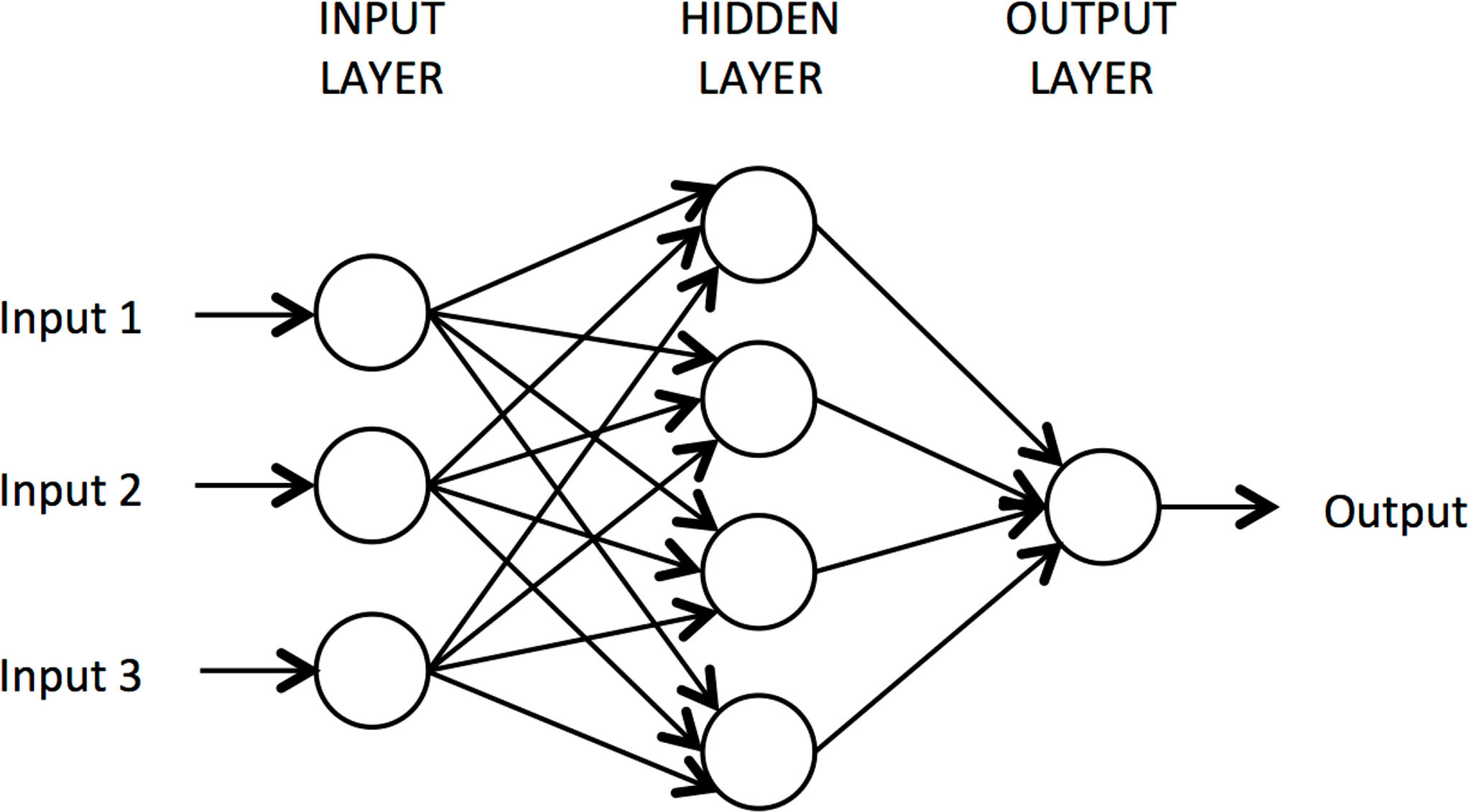
The detailed architecture of the neural network is shown in Figure 2, where the activation function of all of the neurons is the sigmoid function. The number of neurons in the input layer is fixed by the number of input features (one neuron per feature); the same applies for the number of neurons in the output layer, which is one; i.e., the desired probability. For this application, several simulations showed that 10 neurons in the hidden layer provide good accuracy, while also being computationally efficient.
Both the logistic regression and the neural network will provide an output value between 0 and 1 that will represent the probability that a target is located within the sliding window being studied. Thus, a threshold that will determine if an explosive artifact is actually present in each window must also be established. Due to the nature of the problem, the threshold for this application was set very low (0.25), because it is more important to detect everything, even at the cost of an increased rate of false positives, than to obtain false negatives, which would imply that an explosive was not detected and would be dangerous for the demining personnel.
3. Results and Discussion
3.1. Field GPR Data
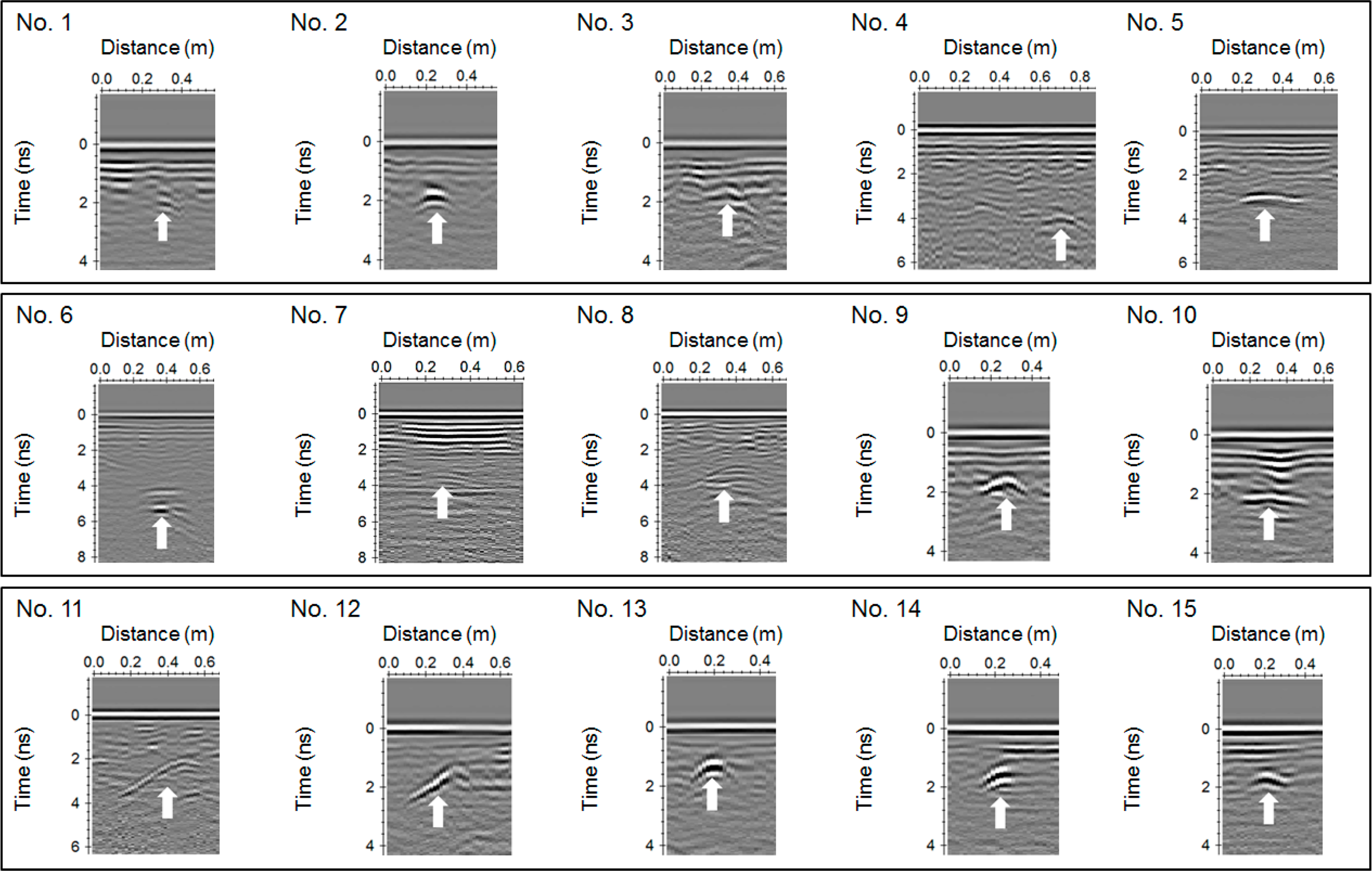
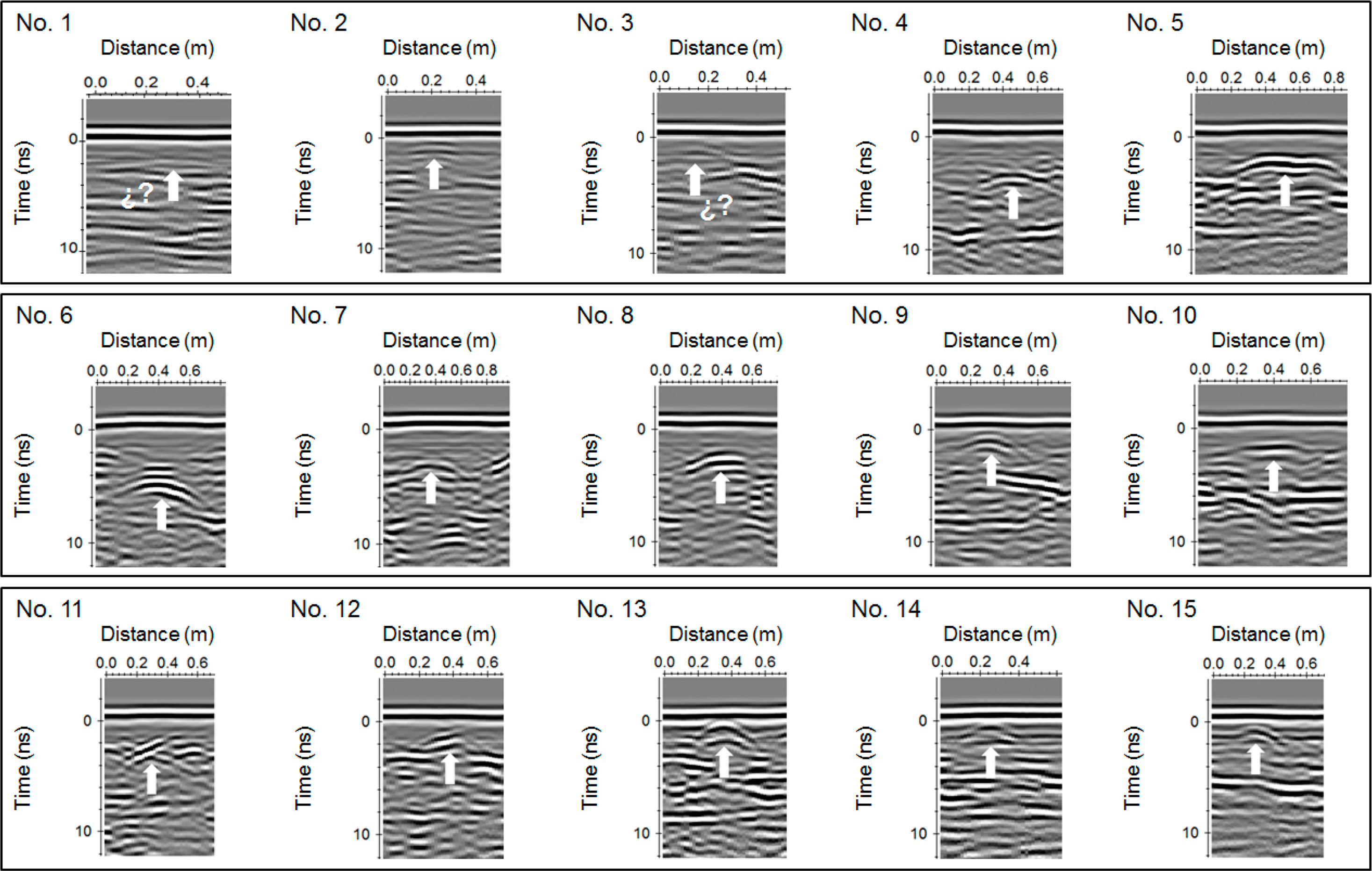
Due to the large number of GPR profile lines that were collected, only the radargrams that show the most interesting reflection from each type of target are shown. Figures 3,4 present the individual portions of the radargrams produced with the 2.3-GHz and 1-GHz antennas, respectively, for each target type.
For the detection of anti-personnel (AP) mines, the signal reflections showed different responses depending on the burial characteristics and the frequency used. The AP mine oriented vertically at a 10-cm depth was identified from the 2.3-GHz data (No. 1 in Figure 3). Nevertheless, the reflection is quite small and is not easily distinguished, due to the minimal thickness of the object, which produces a smaller reflection surface. On the other hand, this object was not identified using the 1-GHz antenna (No. 1 in Figure 4), because of the small size of the object, as well as the lower spatial resolution of the frequency (Table 2) and the near-field antenna coupling induction effects.
For the AP mine that was buried horizontally, hyperbolic reflections were recognized in both the 2.3-GHz and 1-GHz frequencies (No. 2 in Figures 3 and 4, respectively). The reflection pattern is stronger when the target is horizontal, because the reflection surface is larger. The same result is observed for the case of the horizontal anti-tank (AT) mine (No. 6 in Figures 3 and 4). Moreover, in this case, diffractions produced by the presence of air voids can be observed. The experimental scene was created using inert material, which was already exploded and, thus, contained an empty interior space. Reflections generated from the AP mine buried obliquely (No. 2 in Figures 3 and 4) were also detected, but the hyperbolic shape was not perfect, as it was in the previous case. Similar results were found with both vertical AT (No. 7 in Figures 3 and 4) and oblique AT mines (No. 8 in Figures 3 and 4), where the reflection hyperbolas were detected, but were not perfect.
Continuous flat reflections were distinguished for the oblique (Object 4) and horizontal (Object 5) mortar grenades (No. 4,5 in Figures 3 and 4, respectively). The difference in length between the grenades (Table 1) is clearly observed in the radargrams. Similar continuous flat reflections were also obtained with both frequencies from the horizontally buried INSTALAZA II M-63 mortar grenade (No. 10 in Figures 3 and 4). A half-hyperbolic reflection related to the oblique M-63 mortar grenade was obtained using the 2.3-GHz antenna (No. 11 in Figure 3). In contrast, a somewhat continuous reflection was obtained using the 1-GHz antenna (No. 11 in Figure 4). As expected, these results are similar to those obtained for the mortar grenade arranged without the fuse (No. 12 in Table 1), as illustrated in Figures 3 and 4 No. 12.
Hyperbolic reflections were observed for the M-67 metal hand grenade (No. 9 in Figures 3 and 4). The ALHAMBRA-EJ hand grenades, which were buried at depths of 7–10 cm, were also affected by coupling induction effects when surveyed with the 1-GHz antenna. Although this object is mainly composed of plastic, the presence of thin sheet metal produces a stronger signal that facilitates identification (No. 13–15 in Figure 4). Both the vertical (No. 13 in Figures 3 and 4) and horizontal (No. 15 in Figures 3 and 4) grenades showed perfect hyperbolic reflections that were clearly recognized. On the other hand, the obliquely buried grenade showed a half-hyperbola reflection (No. 14 in Figure 3) with the 2.3-GHz data that was not clearly observed in the 1-GHz data (No. 14 in Figure 4).
The metal (perfect reflector) objects showed the strongest signal reflections, due to the greater dielectric contrast with the sandy soils (dielectric constant or K-value of five [19]). However, the plastic objects (K-value of three [33]) were also perfectly detected, although with a lower dielectric contrast. It is important to note that detection of real plastic mines will be better, because they contain metal components; however, real mines were not considered in this study for safety reasons.
3.2. Automated Detection Tool Using Machine Learning Techniques
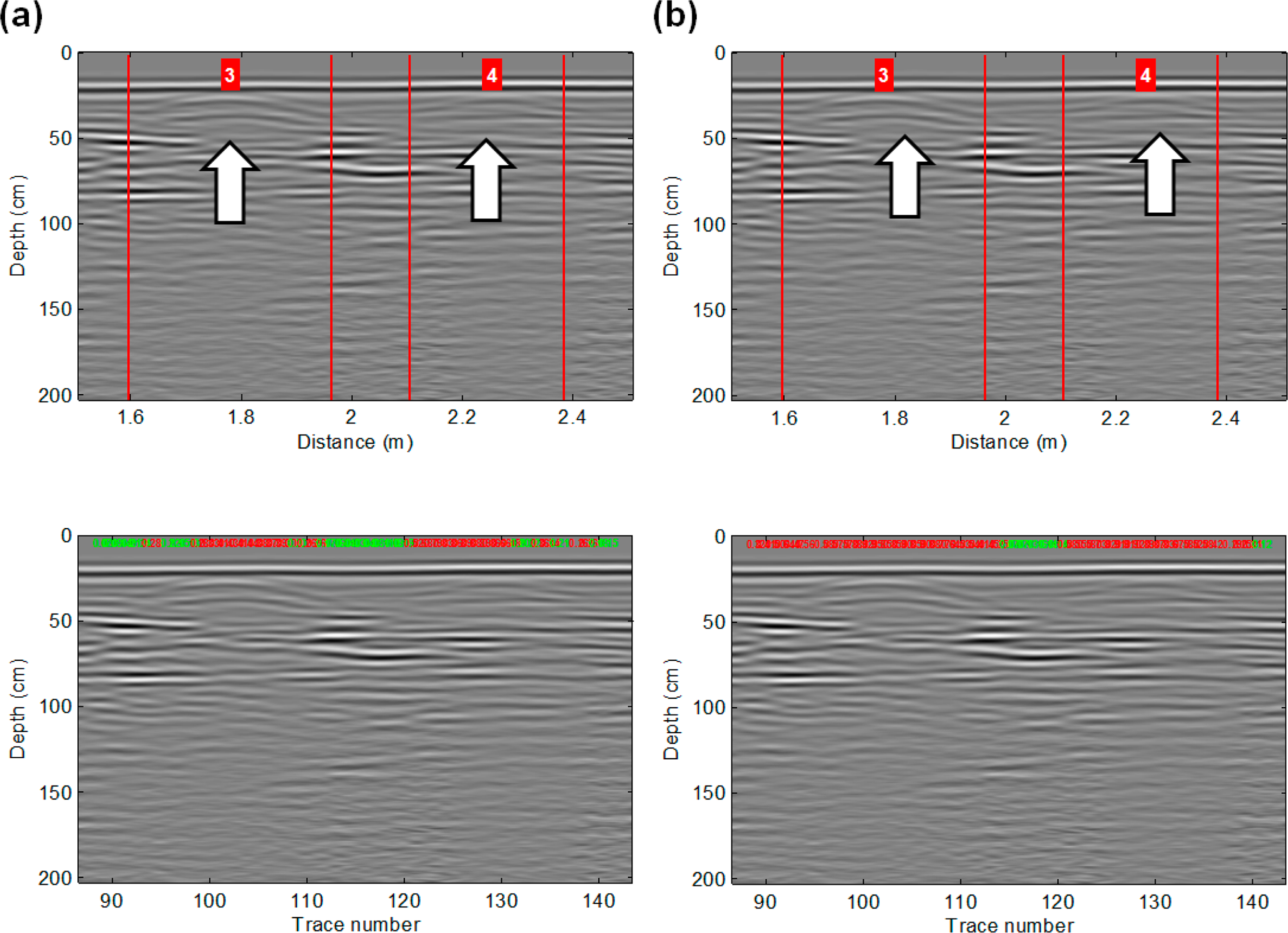
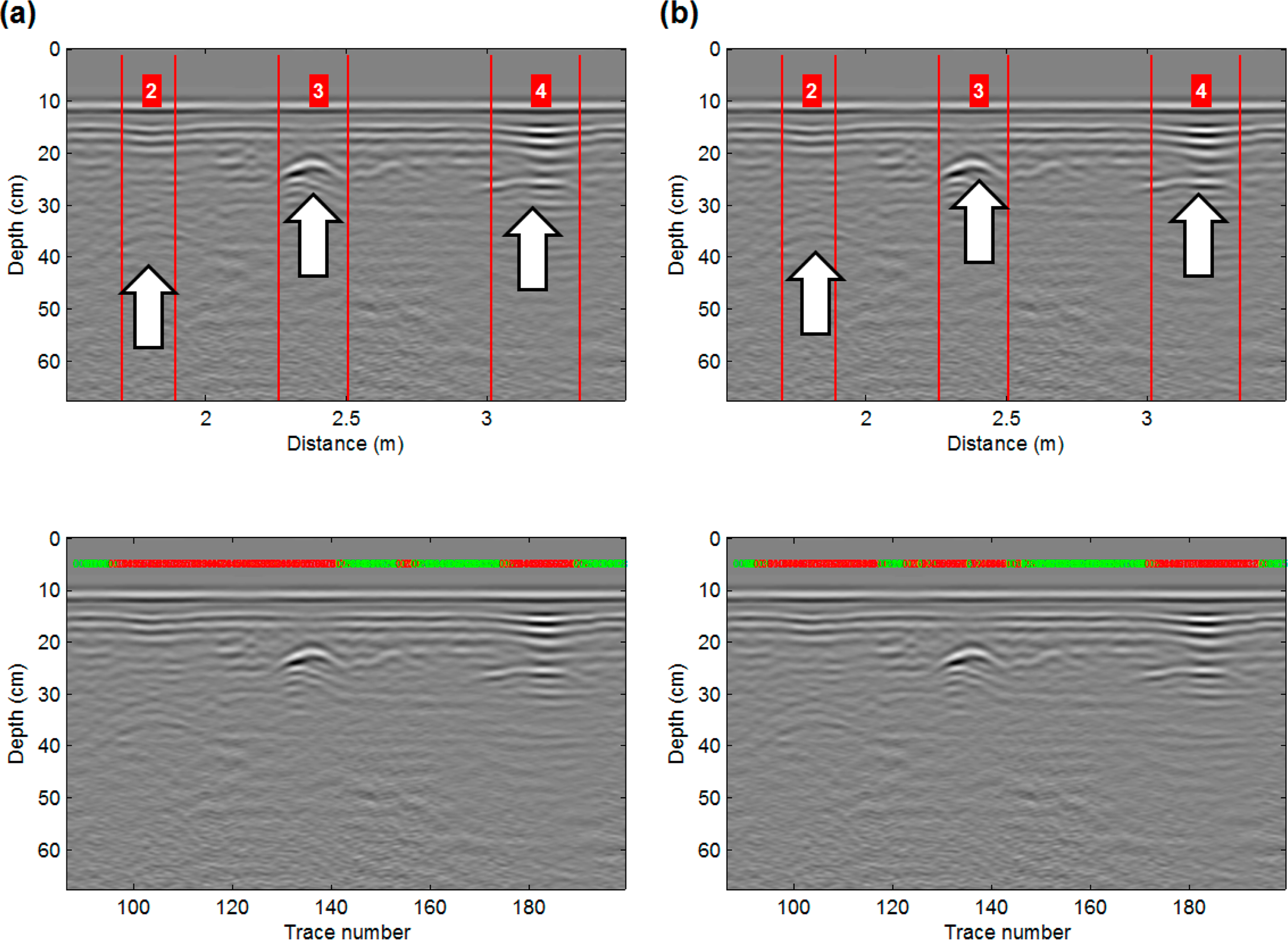
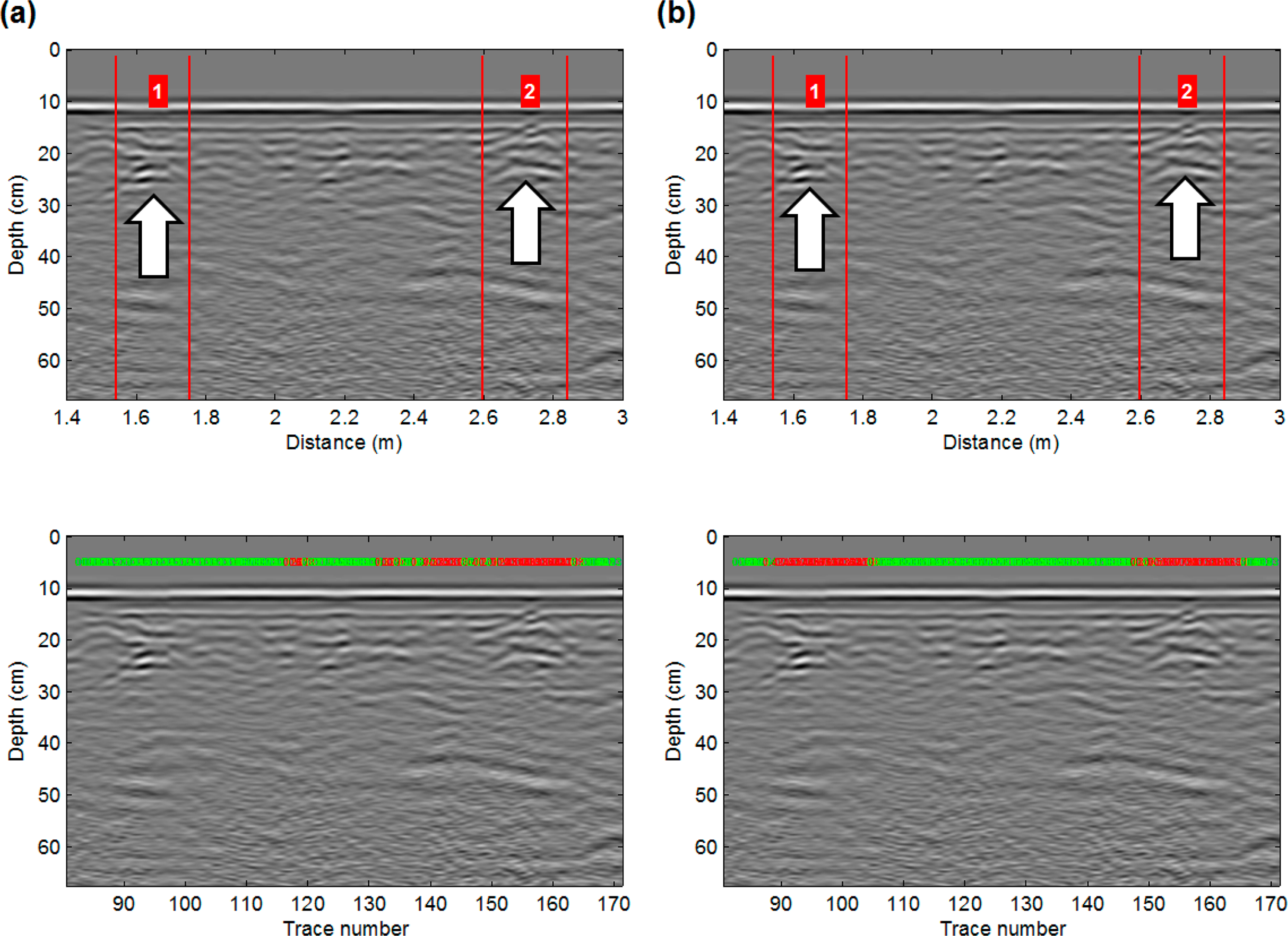
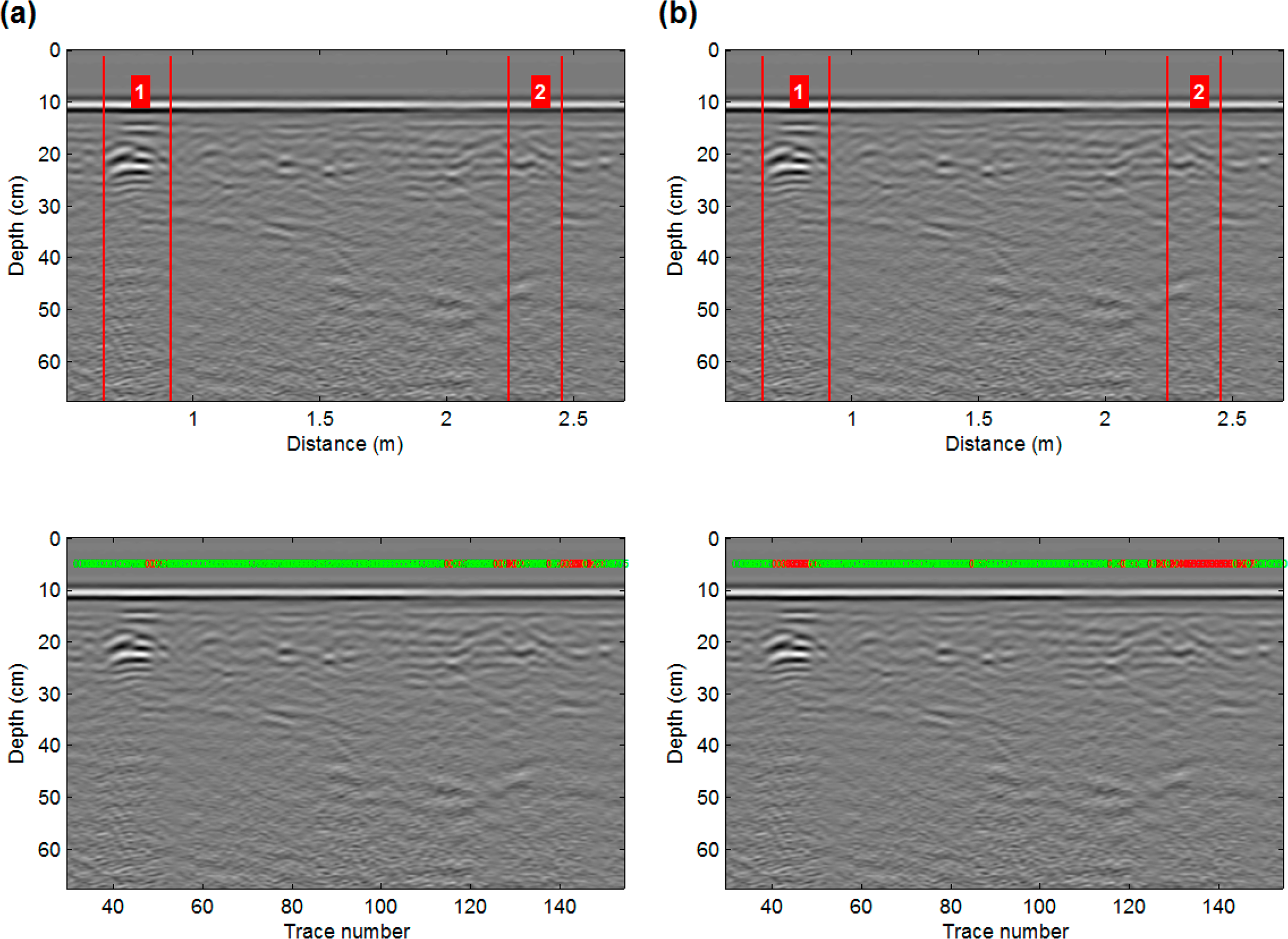
Once systems have been trained, they must be validated by comparing the predictions obtained from the test set with the experimental data. Figure 5 shows an example of how the results are displayed, and Figures 6 and 10 show the results for both the logistic regression and neural network systems for some of the radargrams.
Each figure shows two radargrams; the upper radargram shows where the targets were located, and the lower one shows the outcome of the system for each sliding window; i.e., the probability of an existing target being present within that window. To provide a rapid visual overview, each probability is displayed over its window with a color code that corresponds to the threshold (0.25). Therefore, probabilities displayed in red are those whose values are higher than the threshold, which indicates a high probability of containing a potential target, while green means a low probability.
By comparing the two algorithms, the neural networks were demonstrated to be more accurate and robust than the logistic regressions for both detecting potential explosives and detecting clutter. Figure 6 shows the radargrams of the same profile provided by the two systems with the 1-GHz data, while Figure 7 shows the results for the 2.3-GHz data. The results show that whenever the signal is clear, logistic regression works well.
However, whenever the input signal becomes blurry, the error rate of the logistic regression increases dramatically (Figure 8a). Nevertheless, the neural network remains accurate, even with fuzzy and faint signals (Figure 8b). Remarkably, the neural network provides better spatial resolution and less uncertainty than the logistic regression; i.e., the windows that contain the targets are not as wide as in the regression cases.
Figure 9 shows the outcomes from both systems when dealing with cluttered signals. In these cases, because the clutter provides a fuzzy signal, logistic regression has a high probability of failure (Figure 9a). The neural network remains accurate in these cases, although the probability might experience more spreading among the sliding windows than when detecting solid targets, so the area of high probability will be larger.
Despite the good results, the developed neural network does not have 100% accuracy and might fail in some cases. Figure 10a shows an example of the poor behavior of the network when dealing with a Type 2 target. This target represents an INSTALANZA II M-63 mortar grenade, which happens to be a rare target that appeared in only a few training samples. Because it has a pattern that is completely different from the AP and AT mines, the neural network appears to require additional training samples to be able to recognize it. This is not a failure of the algorithm itself, but is rather a failure of the training set, which is skewed for this type of target.
However, although the network showed some uncertainty in the detection of this type of target (because the area is not completely marked as red), the entire area is not green. This means that the network “has intuition” that something dangerous might be buried in these windows. Thus, coloring the area of uncertainty red serves the final goal of this tool, which is to advise demining personnel of potentially dangerous areas.
The accuracy of the system therefore depends strongly on the quality of the training set. An ideal initial training set should contain as many of the possible targets of interest as possible or at least as many target geometries as possible. If not, the system will be initially skewed, as in this case. However, the system has the ability to learn as it is being used, so a nearly perfect system could be obtained once the network has “seen and learned” the patterns of interest.
On the other hand, when the training samples are not skewed, the neural networks have shown the ability to learn beyond the scope of the targets that were labeled by the programmer. Figure 10b illustrates how the network is able to recognize the faint patterns of an anti-tank mine and a mortar grenade in this profile, even when the programmer discarded them for not being sufficiently clear. This demonstrates how these techniques might be useful for demining technicians to locate and identify potentially dangerous areas where ERW might be buried.
The behaviors of both algorithms in terms of detection percentages are presented in Table 4. The accuracy represents the samples that were properly predicted, including samples that were labeled as targets, noise and clutter. The error rate refers to the samples that were misclassified both as targets and as noise or clutter. The error itself does not provide much information, so it has been divided into two error rates, the false positive rate and the false negative error rate, which are the critical parameters for demining applications.
The false positive rate is composed of those samples that contain noise and that are labeled as potential explosives. This misclassification would lead to additional work for the demining personnel, because they might have to investigate more areas than are needed, but this is not dangerous, because the areas are actually safe. However, the false negative rate represents the percentage of windows that contain an explosive artifact, but are classified as safe. This is the most important parameter for this application, because an area that has been labeled as safe when it is not represents a potential danger during the demining process.
As is shown in Table 4, neural networks are more suitable for this type of problem. They show a high probability of detection, while reducing the probability of false positives and, more importantly, false negatives. The probability of a false positive remains at 4% for both frequencies. This might be due to the limited size of the training set, especially in terms of windows that contain the different types of clutter and special explosive remains, such as the INSTALAZA II M-63 mortar grenade described previously. This means that this problem could be easily solved by adding more samples to the training set to reduce the false positive rate.
However, one of the advantages of machine learning systems over traditional programming is the ability to dynamically learn new features as they are used. Thus, this false negative rate should be considered a maximum-error rate that will only decrease with continued use of the system, thus validating the goal of this paper of using these techniques to automatically detect buried explosives.
The probabilities obtained demonstrate that this system could be useful in a true demining context, especially with the 2.3-GHz antenna, and demonstrate the superiority of the neural network method over other machine learning algorithms, such as logistic regressions.
To improve the results, additional research could be conducted to characterize each type of clutter signal. This study focused on the mine detection algorithm, but to be able to distinguish among different types of UXOs, a more extensive measurement campaign should be carried out.
One limitation of the developed system is that it was only trained with one type of soil. Therefore, an interesting improvement of the learning algorithm might consider the type of soil as an input feature for the system, which could be configured by the user.
A possible solution to the lack of samples and targets might be using finite-difference time-domain (FDTD) simulation methods to increase the diversity (and quantity) of the training set by artificially creating targets and samples on-demand. However, this was not done in this study, because the main goal was to demonstrate how a system that is trained with real samples might be useful in a real demining scenario (Table 4). Because the FDTD signal is cleaner than real signals, better detection probabilities and lower error rates might be expected.
4. Conclusions
This study analyzed the effectiveness of a GPR system in detecting landmines and UXOs. Experimental grids were designed to simulate the most common landmine field scenarios. High-frequency antennas (2.3 GHz and 1 GHz) were used to characterize the most appropriate radar wave responses. In addition, an artificial intelligence approach based on machine learning techniques was considered with the goal of automatically detecting the targets.
Using a methodical, but simple data processing technique, the GPR method is shown to be a suitable method for demining research. The obtained results demonstrate that the combination of 2.3-GHz and 1-GHz frequencies allows for the best evaluation procedure. The 2.3-GHz antenna is the ideal choice for detecting shallow anti-personnel landmines. Deeper anti-tank mines are identified more clearly using the 1-GHz antenna. The experiment was carried out using inert material that did not contain ammunition and any metal components. Therefore, the detection and identification of the targets would increase in real scenarios, due to the larger dielectric contrast between the metal and the sandy soil environment.
Although promising, this technology has limitations, because the resolution required to detect small objects involves GHz frequencies that have low soil penetration and high levels of image clutter. Therefore, the main challenge for detection is further reducing the rate of false alarms. In this sense, this paper presents a novel approach in GPR signal processing by using machine learning techniques to detect buried ERW. Our goal was to develop an automated, fast and real-time detection tool to reduce the false alarm rates and increase the probability of detection to improve the efficiency of demining operations. The ability to extract patterns of clutter and explosive artifacts was tested using logistic regressions and neural networks. Both algorithms showed the ability to discriminate among potential targets and clutter, but the neural network technique is a more robust algorithm in terms of the accuracy and the false positive and false negative error rates. The results also showed the limitations of logistic regressions when dealing with GPR signals, although it is a commonly used classification technique in biostatistics and medicine.
The study also showed that a larger set of training samples is needed to be able to discriminate between the different types of targets and clutter and to reduce the error rate. Finally, the accuracies of both machine learning techniques might improve as they are used, so the percentages shown in Table 4 should be regarded as the lower limits of the capabilities of the algorithms, which addresses the goal of this paper.
Finally, it must be noted that the main focus of this research was in developing a methodology specifically for sandy soil. In the future, this approach will be extended for other common environments involving mining and UXO clearance, namely mountainous terrain, marshy ground, clayey soil, etc.
Acknowledgments
The Defense University Center and the Spanish Military Naval Academy are acknowledged for the facilities and human resources that made this research possible. The authors would also like to acknowledge the support provided by the Applied Geotechnologies Research Group of the University of Vigo. This study is a contribution to the EU-funded Cooperation in Science and Technology COST Action TU-1208 “Civil Engineering Applications of Ground Penetrating Radar”.
Author Contributions
All authors contributed extensively to the work presented in the manuscript.
Conflicts of Interest
The authors declare no conflict of interest.
References
- Banks, E. Brassey’s Essential Guide to Anti-Personnel Landmines; Recognising and Disarming; Brassey’s Ltd.: London, UK, 1997. [Google Scholar]
- Kowalenko, K. Saving lives, one land mine at a time. IEEE Inst 2004, 28, 10–11. Available online: http://theinstitute.ieee.org/ns/quarterly_issues/timar04.pdf (accessed on 21 May 2014). [Google Scholar]
- Joynt, V.P. Mobile metal detection: A field perspective. In Proceedings of 1998 the 2nd International Conference on the Detection of Abandoned Land Mines, Edinburgh, UK, 12–14 October 1998; pp. 14–18.
- Gader, P.D.; Mystkowski, M.; Zhao, Y. Landmine detection with ground penetrating radar using hidden Markov models. IEEE Trans Geosci Remote Sens 2001, 36, 1231–1244. [Google Scholar]
- Daniels, D.J. A review of GPR for landmine detection. Sens Imaging 2006, 7, 90–123. [Google Scholar]
- Daniels, D.J.; Curtis, P. MinehoundTM Trials in Cambodia, Bosnia, and Angola. In Proceedings of 2006 Defense and Security Symposium, Orlando, FL, USA, 17–23 April 2006; p. 62172N.
- Armada, M.; Fernández, R.; Montes, H.; Sarria, J.; Salinas, J.; Salinas, C. Robots Móviles para tareas de desminado humanitario; Universidad Nacional de Educación a Distancia: Madrid, España, 2013; pp. 109–123. [Google Scholar]
- Doheny, R.C. Handheld Standoff Mine Detection System (HSTAMIDS) field evaluation in Namibia. In Proceedings of 2006 Defense and Security Symposium, Orlando, FL, USA, 17–23 April 2006; p. 62172K.
- Dreiseitla, S.; Ohno-Machadob, L. Logistic regression and artificial neural network classification models: A methodology review. J Biomed Inform 2002, 35, 352–359. [Google Scholar]
- Komarek, P. Logistic Regression for Data Mining and High-Dimensional Classification; Carnegie Mellon University: Pittsburgh, PA, USA, 2004; pp. 22–25. [Google Scholar]
- Joseph, P.J.; Vaswani, K.; Thazhuthaveetil, M.J. Construction and use of linear regression models for processor performance analysis. In Proceedings of 2006 Symposium on High Performance Computer Architecture, Austin, TX, USA, 11–15 February 2006; pp. 99–108.
- Plett, G.L.; Doi, T.; Torrieri, D. Mine detection using scattering parameters and an artificial neural network. IEEE Trans. Neural Networks 1997, 8, 1456–1467. [Google Scholar]
- Sheedvash, S.; Azimi-Sadjadi, M.R. Structural adaptation in neural networks with application to land mine detection. In Proceedings of 1997 International Conference on Neural Networks, Houston, TX, USA, 9–12 June 1997; pp. 1443–1447.
- Abdelbaki, H.; Gelenbe, E. Random neural network filter for land mine detection. In Proceedings of 1999 National Radio Science Conference, Cairo, Egypt, 23–25 February 1999; pp. C43/1–C4310.
- Filippidis, A.; Jain, L.C.; Martin, N.M. Using genetic algorithms and neural networks for surface land mine detection. IEEE Trans. Signal Process 1999, 47, 176–186. [Google Scholar]
- Abujarad, F.; Nadim, G.; Omar, A. Clutter reduction and detection of landmine objects in ground penetrating radar data using Singular Value Decomposition (SVD). In Proceedings of 2005 International Workshop on Advanced Ground Penetrating Radar, Delft, The Netherlands, 2–3 May 2005; pp. 37–42.
- Miller, T.W.; Borchers, B.; Hendrickx, J.M.H.; Hong, S-H.; Dekker, L.W.; Ritsema, C.J. Effects of soil physical properties on GPR for landmine detection. In Proceedings of 2001 International Symposium on Technology and the Mine Problem, Monterey, CA, USA, 21–25 April 2002; p. 10.
- Annan, P. Ground Penetrating Radar Principles, Procedures & Applications; Sensors & Software Inc.: Mississauga, ON, Canada, 2003; p. 286. [Google Scholar]
- Daniels, D.J. Ground Penetrating Radar; Institution of Electrical Engineering: London, UK, 2004. [Google Scholar]
- Rial, F.I.; Pereira, M.; Lorenzo, H.; Arias, P.; Novo, A. Resolution of GPR bowtie antennas: An experimental approach. J. Appl. Geophys 2009, 67, 367–373. [Google Scholar]
- Pérez-Gracia, V.; Di Capua, D.; González-Drigo, R.; Pujades, L. Laboratory characterization of a GPR antenna for high-resolution testing: Radiation pattern and vertical resolution. NDT & E International 2009, 42, 336–344. [Google Scholar]
- Jol, H.M. Ground Penetrating Radar: Theory and Applications; Elsevier: Amsterdam, The Netherlands, 2009; pp. 3–40. [Google Scholar]
- Tesfamariam, G.T.; Dilip, M. Application of advanced background subtraction techniques for the detection of buried plastic landmines. Int J Emerg Technol Adv Eng 2014, 4, 318–323. [Google Scholar]
- Gonzalez-Huici, M.A.; Giovanneschi, F. A combined strategy for landmine detection and identification using synthetic GPR responses. J Appl Geophys 2013, 99, 154–165. [Google Scholar]
- Dyana, A.; Rao, C.H.; Kuloor, R. 3D segmentation of ground penetrating radar data for landmine detection. In Proceedings of 2012 International Conference on Ground Penetrating Radar, Shanghai, China, 4–8 June 2012; pp. 858–863.
- Deiana, D.; Anitori, L. Detection and classification of landmines using AR modeling of GPR data. In Proceedings of 13th International Conference on Ground Penetrating Radar, Lecce, Italy, 21–25 June; 2010. [Google Scholar] [CrossRef]
- Shi, Y.; Song, Q.; Jin, T.; Zhou, Z. Landmine detection using boosting classifiers with adaptive feature selection. In Proceedings of 2011 International Workshop on Advanced Ground Penetrating Radar, Aachen, Germany, 22–24 June 2011; pp. 1–5.
- Bishop, C.M. Neural Networks for Pattern Recognition; Clarendon Press: Oxford, UK, 1995; pp. 116–161. [Google Scholar]
- Sandmeier, K.J. ReflexW Manual. Available online: http://www.sandmeier-geo.de (accessed on 21 May 2014).
- Khan, U.S.; Al-Nuaimy, W. Background removal from GPR data using eigenvalues. In Proceedings of 2010 the 13th International Conference on Ground Penetrating Radar, Lecce, Italy, 21–25 June 2010. [CrossRef]
- Abdullah-Al-Wadud, M.; Hasanul-Kabir, M.; Ali-Akber-Dewan, M.; Chae, O. A dynamic histogram equalization for image contrast enhancement. IEEE Trans Consum Electron 2007, 53, 593–600. [Google Scholar]
- Van der Merwe, A.; Gupta, I.J. A novel signal processing technique for clutter reduction in GPR measurements of small, shallow land mines. IEEE Trans Geosci Remote Sens 2000, 38, 2627–2637. [Google Scholar]
- Pérez-Gracia, V. Radar de Subsuelo. Evaluación para aplicaciones en arqueología y en patrimonio artístico. Ph.D. thesis, Polytechnic University of Catalonia, Barcelona, Spain. 2001. [Google Scholar]


| Nº | Object | Designation | Image | Dimensions | Casing | Depth | Orientation |
|---|---|---|---|---|---|---|---|
| 1 | Anti-personnel mine | AP-SB33 |  | t = 3.23 cm Ø = 8.46 cm | Plastic | 10 cm | Vertical |
| 2 | Horizontal | ||||||
| 3 | Oblique | ||||||
| 4 | Mortar grenade | GM-ECIA |  | L = 26 cm Ø = 5.98 cm | Metal | 20 cm | |
| 5 |  | L = 38 cm Ø = 7.86 cm | Horizontal | ||||
| 6 | Anti-tank mine | AT-SB81 |  | t = 10 cm Ø = 22 cm | Plastic | 30 cm | |
| 7 | 25 cm | Vertical | |||||
| 8 | Oblique | ||||||
| 9 | Hand grenade | M-67 |  | L = 9.31 cm Ø = 6.14 cm | Metal | 12 cm | Horizontal |
| 10 | Mortar grenade | INSTALAZA II M-63 |  | L = 34.5 cm Ø = 3.56 cm | Metal | 15 cm | Horizontal |
| 11 | Oblique | ||||||
| 12 |  | L = 31 cm Ø = 3.56 cm | 10 cm | ||||
| 13 | Hand grenade | ALHAMBRA-EJ |  | L = 7.54 cm Ø = 6.37 cm | Plastic | Vertical | |
| 14 | 7 cm | Oblique | |||||
| 15 | Horizontal | ||||||
| GPR Antenna | Max Depth (m) | Δt (ns) | Vertical Resolution (Rv) (cm) | Horizontal Resolution (Rh) (cm) | ||
|---|---|---|---|---|---|---|
| 10 cm | 20 cm | 30 cm | ||||
| 2.3 GHz | 0.5 | 0.435 | 4 | 17 | 23 | 27 |
| 1 GHz | 1.5 | 1 | 9 | 28 | 36 | 43 |
| 800 MHz | 2.5 | 1.25 | 12 | 31 | 41 | 48 |
| 500 MHz | 6.0 | 2 | 19 | 43 | 55 | 63 |
| 2.3 GHz | 1 GHz |
|---|---|
| 1. Time-zero correction | 1. Time-zero correction |
| 2. Dewow filtering (time window: 0.5 ns) | 2. Dewow filtering (time window: 1 ns) |
| 3. Gain function (linear: 5; exponential: 4) | 3. Gain function (linear: 2; exponential: 1) |
| 4. Subtracting average (average traces: 200) | 4. Subtracting average (average traces: 200) |
| Accuracy | Error Rate | |||
|---|---|---|---|---|
| False Positive | False Negative | |||
| Logistic Regression | 1 GHz | 57% | 28% | 15% |
| 2.3 GHz | 65% | 17% | 18% | |
| Neural Network | 1 GHz | 89% | 7% | 4% |
| 2.3 GHz | 92% | 4% | 4% | |
© 2014 by the authors; licensee MDPI, Basel, Switzerland This article is an open access article distributed under the terms and conditions of the Creative Commons Attribution license (http://creativecommons.org/licenses/by/4.0/).
Share and Cite
Núñez-Nieto, X.; Solla, M.; Gómez-Pérez, P.; Lorenzo, H. GPR Signal Characterization for Automated Landmine and UXO Detection Based on Machine Learning Techniques. Remote Sens. 2014, 6, 9729-9748. https://doi.org/10.3390/rs6109729
Núñez-Nieto X, Solla M, Gómez-Pérez P, Lorenzo H. GPR Signal Characterization for Automated Landmine and UXO Detection Based on Machine Learning Techniques. Remote Sensing. 2014; 6(10):9729-9748. https://doi.org/10.3390/rs6109729
Chicago/Turabian StyleNúñez-Nieto, Xavier, Mercedes Solla, Paula Gómez-Pérez, and Henrique Lorenzo. 2014. "GPR Signal Characterization for Automated Landmine and UXO Detection Based on Machine Learning Techniques" Remote Sensing 6, no. 10: 9729-9748. https://doi.org/10.3390/rs6109729
APA StyleNúñez-Nieto, X., Solla, M., Gómez-Pérez, P., & Lorenzo, H. (2014). GPR Signal Characterization for Automated Landmine and UXO Detection Based on Machine Learning Techniques. Remote Sensing, 6(10), 9729-9748. https://doi.org/10.3390/rs6109729