An Analysis of the Side Slither On-Orbit Calibration Technique Using the DIRSIG Model

Abstract

Pushbroom-style imaging systems exhibit several advantages over line scanners when used on space-borne platforms as they typically achieve higher signal-to-noise and reduce the need for moving parts. Pushbroom sensors contain thousands of detectors, each having a unique radiometric response, which will inevitably lead to streaking and banding in the raw data. To take full advantage of the potential exhibited by pushbroom sensors, a relative radiometric correction must be performed to eliminate pixel-to-pixel non-uniformities in the raw data. Side slither is an on-orbit calibration technique where a 90-degree yaw maneuver is performed over an invariant site to flatten the data. While this technique has been utilized with moderate success for the QuickBird satellite [1] and the RapidEye constellation [2], further analysis is required to enable its implementation for the Landsat 8 sensors, which have a 15-degree field-of-view and a 0.5% pixel-to-pixel uniformity requirement. This work uses the DIRSIG model to analyze the side slither maneuver as applicable to the Landsat sensor. A description of favorable sites, how to adjust the maneuver to compensate for the curvature of “linear” arrays, how to efficiently process the data, and an analysis to assess the quality of the side slither data, are presented.

1. Introduction

Traditional line scanners used on space-borne platforms (e.g., MODIS and ETM+) contain a handful of detectors that collect data of a scene in the cross-track direction as the satellite flies over in the along-track direction [3,4]. Minimal effort is required to perform a relative calibration of their data as the simplicity of their focal plane design minimizes non-uniformities in the raw data [5]. However, these sensors require moving parts, which have the potential to fail on-orbit, and exhibit relatively low signal-to-noise ratios (SNR) compared to modern pushbroom systems. The focal plane design of pushbroom-style architectures is advantageous as it eliminates the need for cross-track motion when collecting data. As a result, the need for moving parts is reduced and SNR is enhanced due to longer dwell times [6]. To take full advantage of these potential benefits, much more effort is required to perform a relative calibration as pushbroom sensors typically contain tens-of-thousands (if not hundreds-of-thousands) of detectors arranged on several focal plane modules (FPMs) that are staggered across the focal plane [7].

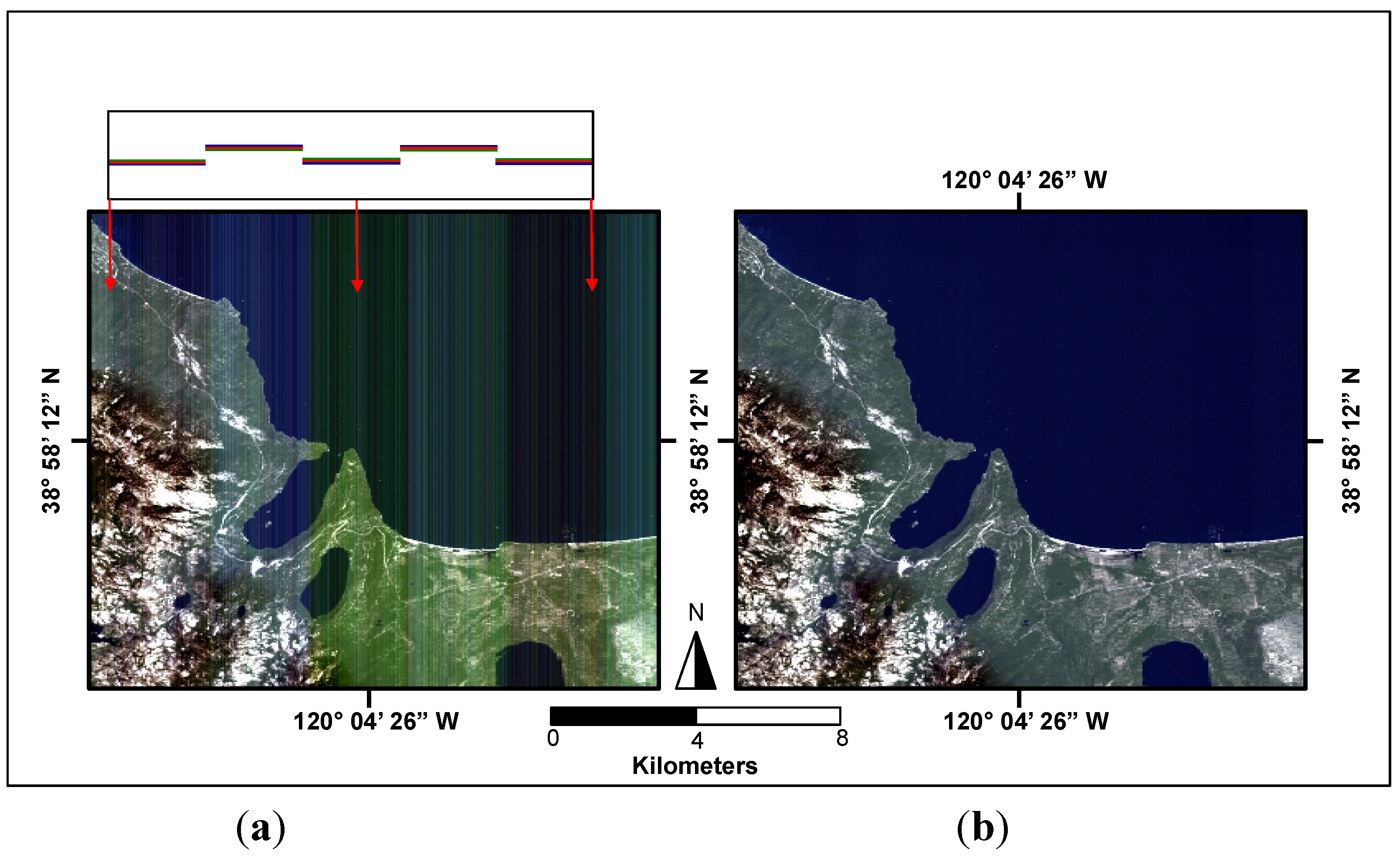
Figure 1 shows a generic focal plane design for a pushbroom sensor and the raw data (simulated in this case) that is collected from this type of system. Each detector on the focal plane will have a unique radiometric response due to the doping process used to fabricate the detector arrays, variability in electronic gains and biases, and lens fall-off. As a result, banding and streaking will be apparent in the raw data and must be corrected, so as to take full advantage of the enhanced SNR exhibited by these modern imaging systems. Figure 1a shows the raw simulated image data prior to calibration while Figure 1b shows the processed data after flat-fielding.

Figure 1. Focal plane design of a typical pushbroom sensor used to simulate data of Lake Tahoe, California with all non-uniformity effects applied (i.e., per detector gains, biases, spectral response functions, nonlinearities, noise, etc.) (a) Shows the raw data and (b) shows data after flat-fielding.

Figure 1. Focal plane design of a typical pushbroom sensor used to simulate data of Lake Tahoe, California with all non-uniformity effects applied (i.e., per detector gains, biases, spectral response functions, nonlinearities, noise, etc.) (a) Shows the raw data and (b) shows data after flat-fielding.

The nine-band Operational Land Imager (OLI) and the dual band Thermal Infrared Sensor (TIRS) are the latest sensors in the Landsat series and, in a departure from traditional sensor design, use pushbroom-style architectures. They were launched onboard Landsat 8 (formerly LDCM) on 11 February 2013. OLI is equipped with dual full-aperture solar diffusers and multi-bulbed tungsten lamp assemblies that are used for on-orbit detector-to-detector radiometric calibration. The primary solar diffuser is deployed every eight days to determine flat-fielding coefficients and the pristine diffuser every six months to monitor the primary diffuser’s degradation. Tungsten lamp assemblies will provide an additional source of calibration coefficients; a working lamp set will be used daily, a reference lamp set monthly, and a pristine lamp set every six months [8]. TIRS is equipped with a scene select mechanism that is deployed regularly to view deep space and its onboard blackbody to enable an on-orbit detector-to-detector radiometric calibration [9].

To perform a relative calibration as illustrated in Figure 1, a governing calibration equation relating radiance at the focal plane to digital counts for each detector must be defined. For each detector within an array,

$$D{N}_i=Q\left[G_i·f_i\left(L\right)+B_i\right]; for i=0, 1, \dots , n$$

(1)

where DN_i is the raw detector response in digital counts for detector i, f_i(L) is the radiometric response function of the detector i to the incident radiance, G_i is the gain for detector i, B_i is the bias measured in the absence of light for detector i, n is the total number of detectors in the array, and Q[] indicates the quantization process. Although detectors may have a nonlinear radiometric response, these effects are not directly addressed in this work. Additionally, the bit-depth of most modern sensors is at least 12-bit so Equation (1) can be simplified to,

$$D{N}_i=G_i·L+B_i;fori=0,1,\dots ,n$$

(2)

To perform a relative calibration on-orbit, per-detector biases from Equation (2) can be obtained by imaging deep space or by closing the shutter. Then by sampling a uniform bright source (L_f), per-detector gains can be derived for each detector,

$$\widehat{G_i}=\frac{D{N}_i-B_i}{L_f}; for i=0, 1, \dots , n$$

(3)

The gains from Equation (3) can be divided by the average gain across the entire array to derive the relative gains that get applied during the flat-field correction.

$${\hat{G}}_{r_i}=\frac{{\hat{G}}_i}{\raisebox{1ex}{${{\displaystyle \sum }}^{\text{}}{\hat{G}}_i$}\!\left/ \!\raisebox{-1ex}{$n$}\right.}; for i=0, 1, \dots , n$$

(4)

A flat-field correction can then be obtained in image data by applying Equation (5) for each detector i.

$$D{N}_{ff}=\frac{D{N}_i-B_i}{{\hat{G}}_{r_i}}; for i=0, 1, \dots , n$$

(5)

Note that this procedure must be applied for all arrays on the focal plane. For satellite systems equipped with a solar diffuser, a uniform bright source (L_f) can be achieved by introducing the solar-diffuser into the field-of-view (FOV) of the sensor to flood the focal plane with diffuse, reflected sunlight. However, diffuser panels can degrade over time causing a non-uniform illumination of the focal plane. This is evident with Terra’s MODIS (The Moderate Resolution Imaging Spectroradiometer) sensor where an anomaly forcing its solar diffuser door to remain open has led to an accelerated degradation of its solar diffuser [10]. As a result, the proper performance of the Terra MODIS solar diffuser stability monitor is critical to a well-calibrated system. The OLI is equipped with a pristine diffuser that may be used to monitor the primary diffuser’s degradation but the need for a vicarious method to flat-field the data is desirable for systems not equipped with on-board calibrators.

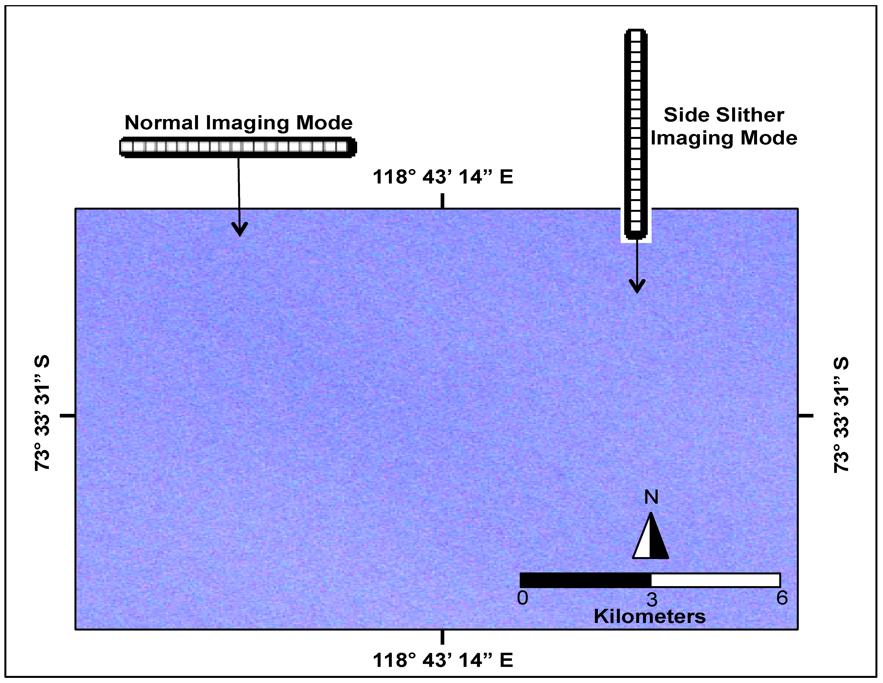
The side slither calibration technique is an on-orbit maneuver that has been used to flat-field image data for the QuickBird and RapidEye pushbroom systems [1,2]. The Earth’s surface exhibits excessive variability to enable a relative calibration in normal imaging mode with wide FOV pushbroom instruments. However, a 90-degree yaw maneuver can be applied to the spacecraft (thus the focal plane) forcing each detector to image a similar spot on the ground. This concept is illustrated in Figure 2 which shows an ideal linear array imaging over Dome Concordia (Dome C), Antarctica in both normal imaging mode (left) and in side slither imaging mode (right).

When the satellite is yawed 90 degrees, each detector on the idealized focal plane array will scan over the same area on the ground. This is a favorable scenario for relative calibration, as each detector should receive the same illumination. However, pushbroom-style imaging systems with wide fields-of-view (e.g., Landsat sensors) are not perfect linear arrays but more closely resemble the array illustrated in Figure 1.

Figure 2. Illustration of a perfect linear array imaging over Dome Concordia, Antarctica in both normal imaging mode and side slither mode.

Figure 2. Illustration of a perfect linear array imaging over Dome Concordia, Antarctica in both normal imaging mode and side slither mode.

This article presents the results of simulated studies designed to investigate the potential to use the side slither maneuver to perform a relative calibration for pushbroom-style imaging systems such as Landsat 8 (i.e., systems with a wide field-of-view). While this technique has been previously applied to other systems, the sources of potential errors in the flat-field process have not been convincingly identified. This work uses simulation and modeling to identify sources that will introduce errors into the calibration process, to assist in developing metrics to evaluate the efficacy of the side slither maneuver, and to provide recommendations for future side slither missions.

Section 2 introduces techniques that enable an enhanced side slither calibration to be performed. Illustrations of how side slither data are obtained, how it can be interpreted, and how it is processed to calculate relative gains are presented. Preprocessing techniques intended to minimize scene-induced error are then presented and a simulated case study designed to identify uniform regions on Earth suitable for the side slither maneuver is introduced. In Section 3, potential issues associated with performing a relative calibration using side slither are identified and on-orbit modifications to the technique suggested. Additionally, a qualitative characterization of how to identify uniform regions that are suitable for the maneuver is provided. The site identification study is revisited and re-designed for sensors with a wide field-of-view. Finally, a summary of the side slither recommendations made for Landsat 8 during its commissioning phase is presented.

2. The Side Slither Maneuver

Before describing the processing chain that can be applied to effectively flat-field an image using the side slither maneuver, a basic knowledge of the data is required. To develop an understanding of the difference between data collected in normal imaging mode and side slither mode, simulation and modeling can be utilized. The DIRSIG (Digital Imaging and Remote Sensing Image Generation) model was used to support this work. DIRSIG is a well-developed physics-based model created at the Rochester Institute of Technology to simulate the spectral radiance images produced by sensors that observe the reflective and emitted energy from the Earth’s surface [11]. DIRSIG supports scenes developed from complex geometries or can use radiance data directly as input to describe the synthetic landscape. Recent enhancements to DIRSIG support the development of a sophisticated data-driven sensor model [12]. If the user is able to make lab measurements, DIRSIG accepts line-of-sight measurements to define the focal plane layout, platform jitter, and can handle inputs of gains, biases, relative spectral response functions, noise, etc. on a per-detector basis [13,14,15].

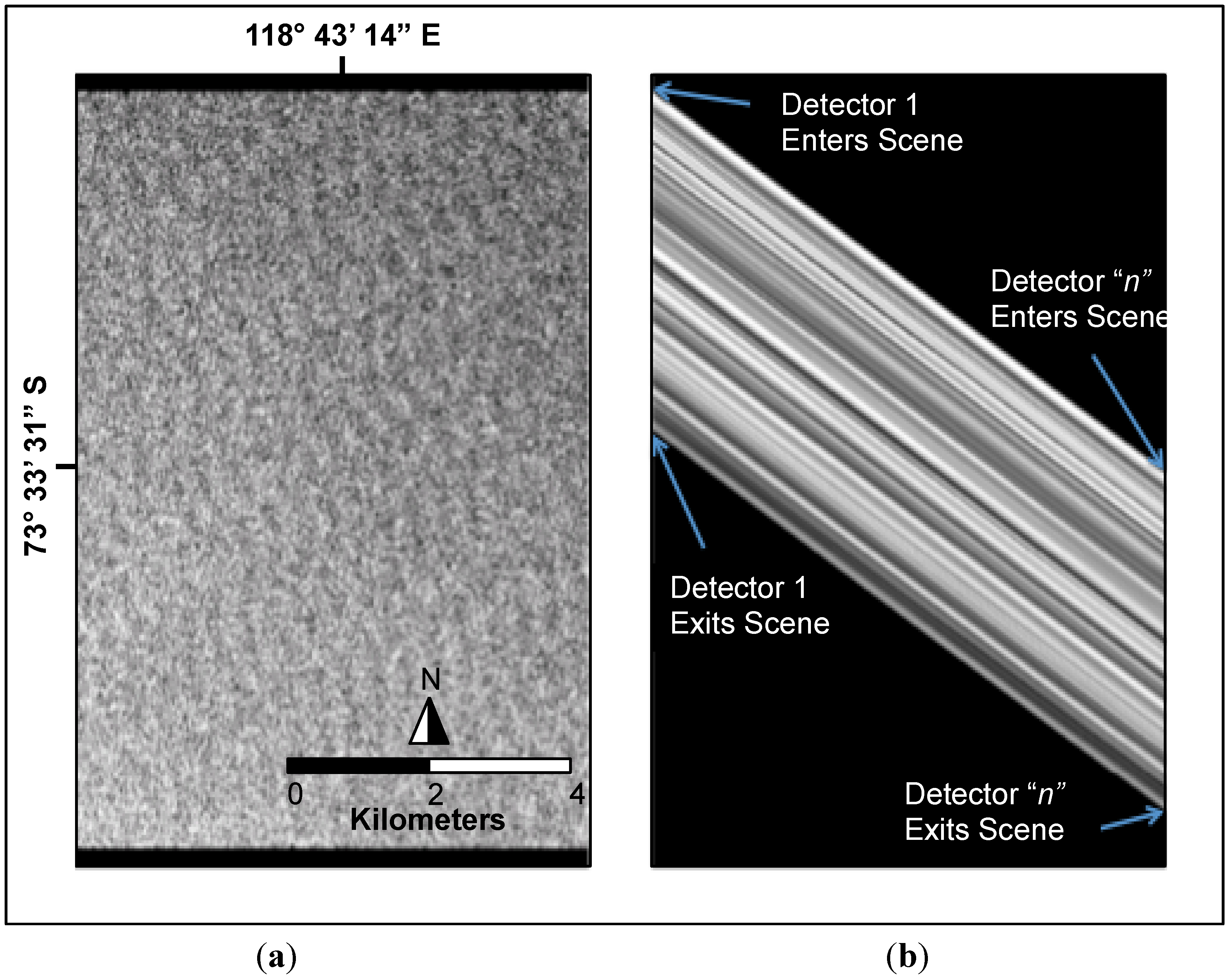
To generate the simulated data shown in Figure 3, Landsat 7 radiance data of the Dome C (from Figure 2) was provided directly as input to the DIRSIG model and imaged using a simple linear array in both normal and side slither imaging modes. Figure 3a shows the data that results from imaging in normal mode while Figure 3b shows the corresponding side slither data (Note: for simplicity the Earth beyond the Dome C “scene” was treated as a black background in these initial DIRSIG simulations).

To develop our knowledge of how the side slither data shown in Figure 3b is obtained, and how it can potentially be used for calibration, we refer again to Figure 2. By treating the Earth outside the scene of interest as a black background, each detector of the linear array will image black prior to entering the uniform region when imaging in side slither mode. This is shown in Figure 3b where the first few rows of the image are black. When the first detector enters the scene, the array images all black except for the first detector (first column in Figure 3b). As subsequent detectors image over the uniform region, more image data is introduced into each column from left to right. Approximately halfway down Figure 3b, the first detector leaves the uniform region as indicated by the introduction of black data in the first column. As subsequent detectors leave the uniform region, black data is introduced to the corresponding columns until finally all detectors image black. The last few rows of Figure 3b indicate that all detectors are imaging outside of the uniform region.

Figure 3. DIRSIG simulated grayscale images collected over Dome Concordia, Antarctica in both (a) normal mode and (b) side slither mode.

Figure 3. DIRSIG simulated grayscale images collected over Dome Concordia, Antarctica in both (a) normal mode and (b) side slither mode.

2.1. Basic Processing

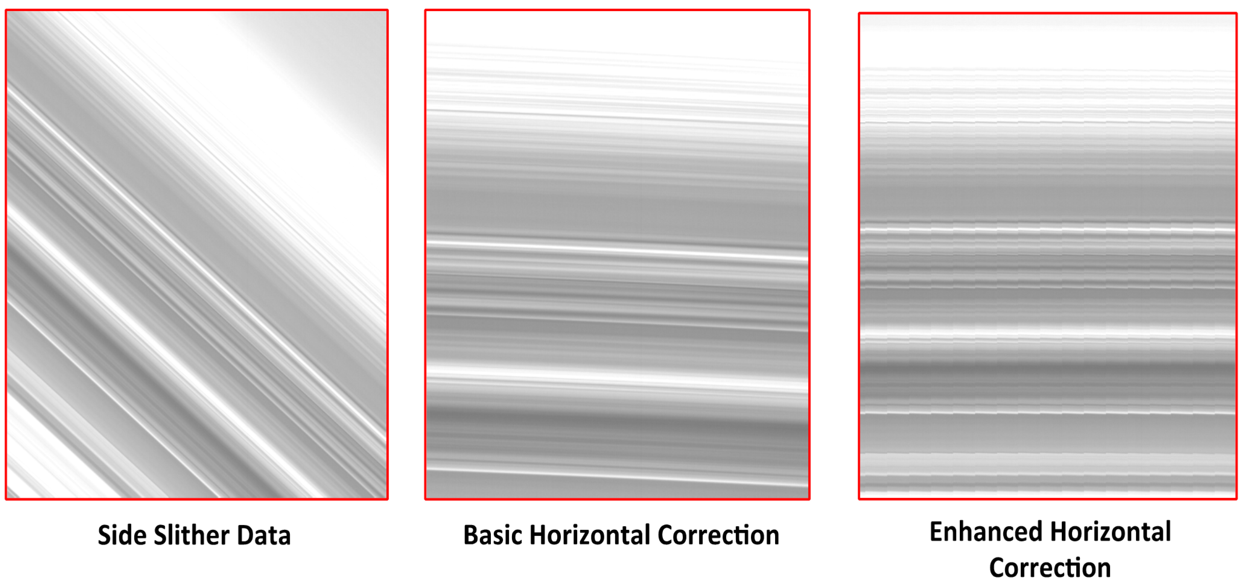
The techniques described in [1] and [2] describe how side slither data should be shifted prior to processing the relative gains. In this paper, a horizontal correction is defined as a shifting of the columns in the side slither data so the linear features in the data are oriented horizontally. A horizontal correction is performed prior to calculating relative gains to simplify the data processing. Figure 4 illustrates the horizontal correction process where each subsequent column i of the raw side slither data (left) is shifted up.

Shift_i = i − 1

(6)

So (according to Equation (6)) the first column of the data is left alone, the second column is shifted up one row, the third column is shifted up two rows, and so on. Figure 4(center) shows the result of this nominal horizontal correction process. Notice that the linear features in the data are not perfectly horizontal. This is likely due to the focal plane read-out clock cycle being out of synch when the array is oriented in the direction of motion, a perfect 90-degree side slither is not achieved, or a combination of the two. Figure 4(right) shows the side slither data after an enhanced horizontal correction has been applied, where the slopes of the lines in Figure 4(center) were determined and used to further shift the data. Note that in the enhanced correction, only integer shifts of the data are applied to avoid the resampling of data.

Figure 4. Illustration of the horizontal correction process where raw Thermal Infrared Sensor (TIRS) side slither data (left) was corrected using a nominal correction (center) and an enhanced correction (right).

Figure 4. Illustration of the horizontal correction process where raw Thermal Infrared Sensor (TIRS) side slither data (left) was corrected using a nominal correction (center) and an enhanced correction (right).

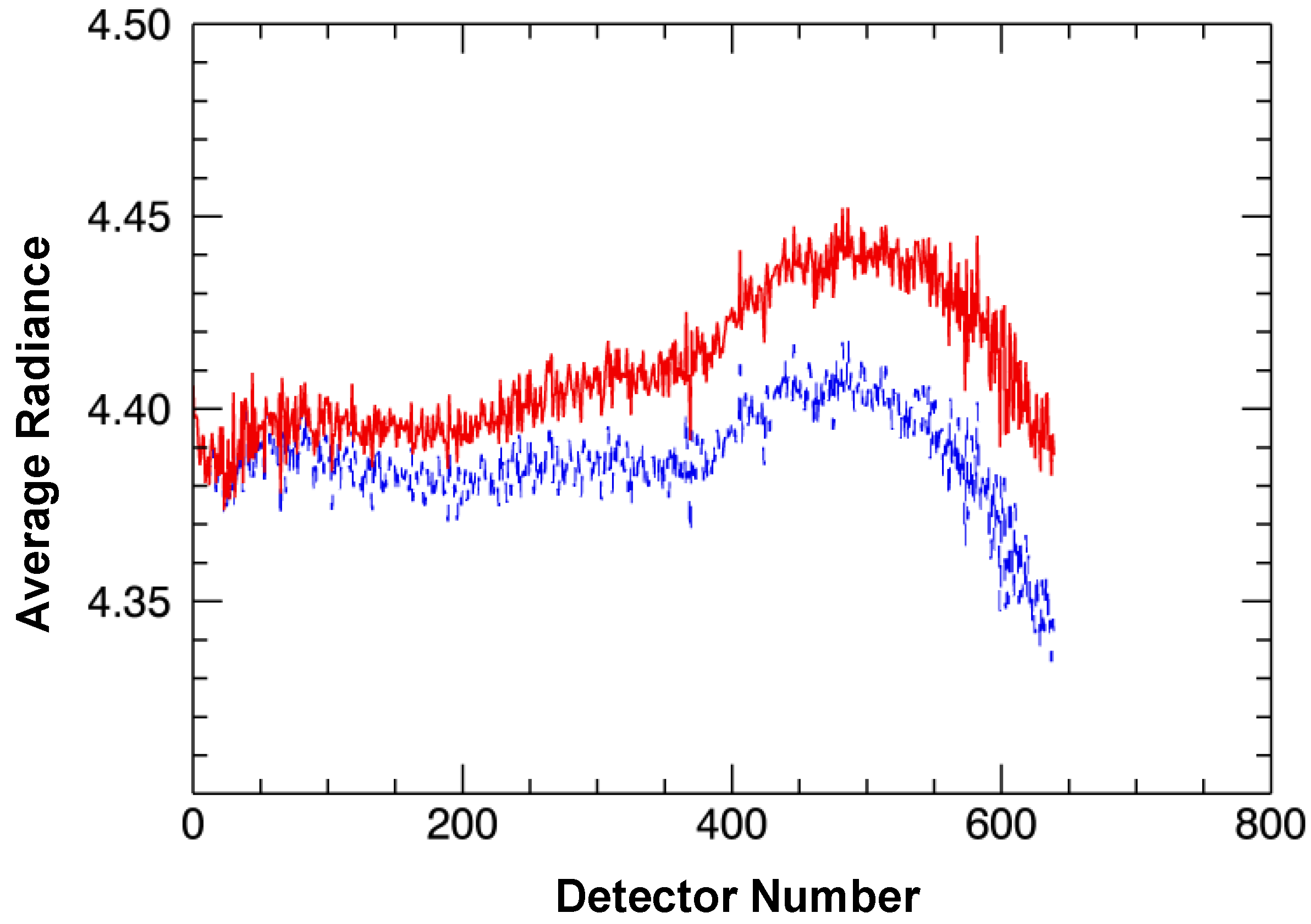
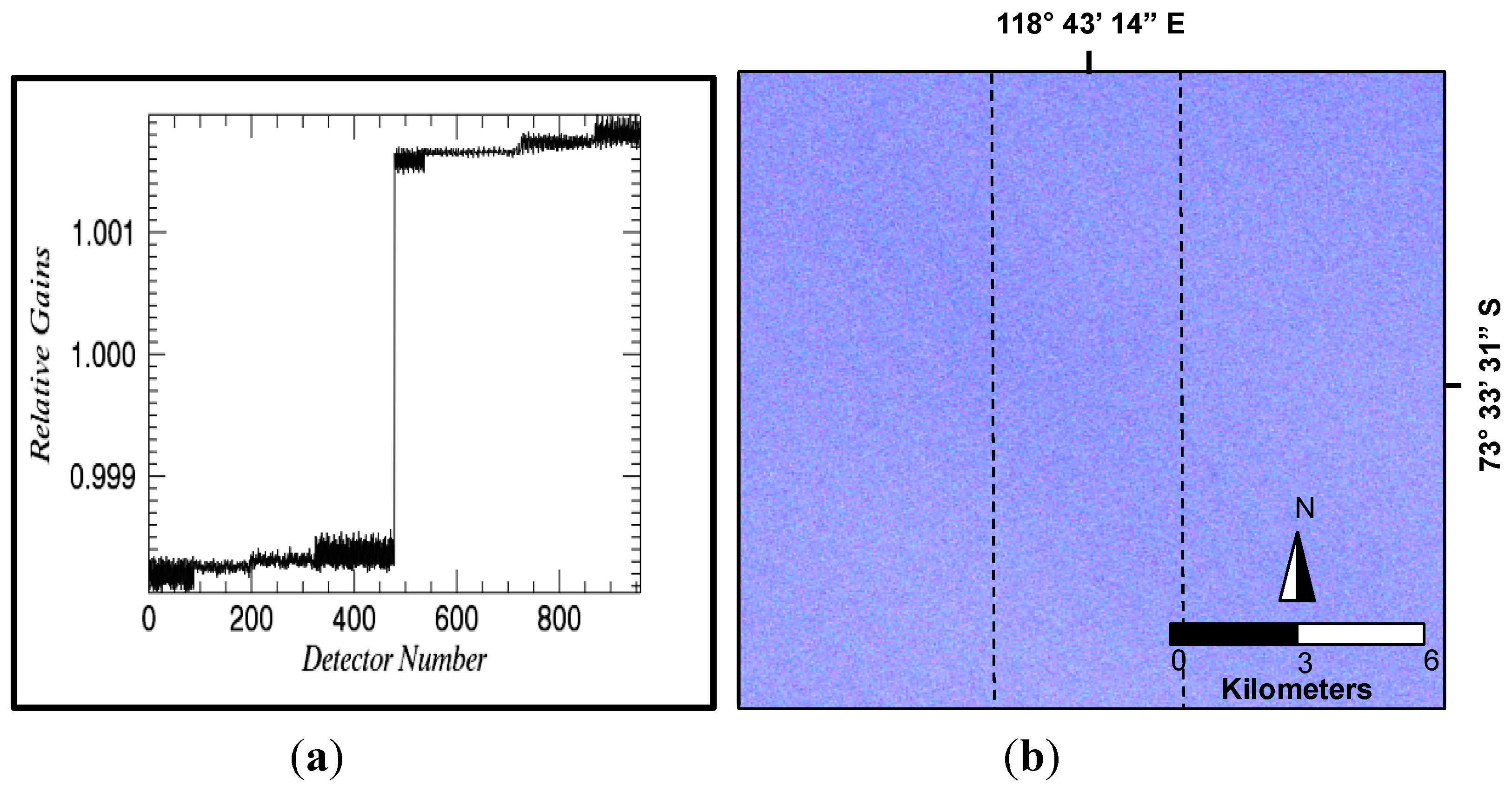
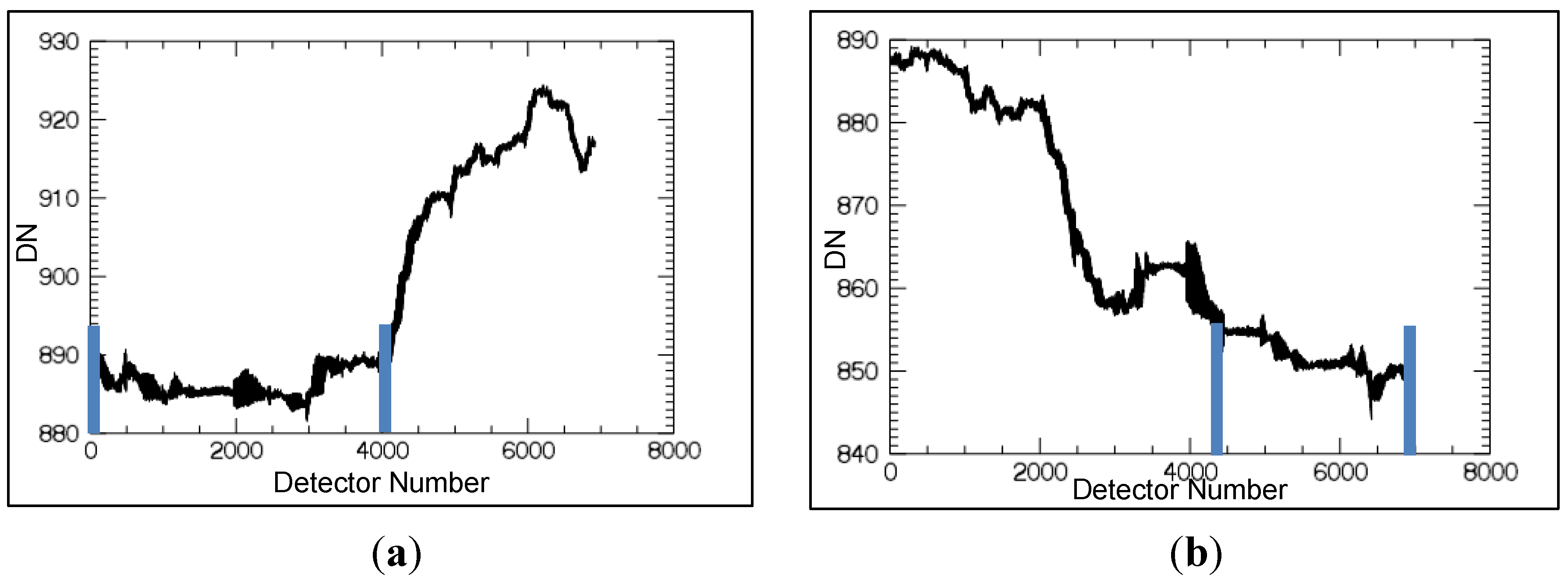
The enhanced correction is a manual process, as conducted in this research, but potentially significant to an accurate relative calibration. Figure 5 shows the column averages of the side slither data from Figure 4. The red (solid) curve in Figure 5 corresponds to the column average for each detector calculated from the side slither data when a basic horizontal correction is applied, i.e., Figure 4 (center). The blue (dashed) curve corresponds to the column averages when the enhanced horizontal correction is applied, Figure 4(right). The two curves differ by as much as 1.5 percent in this example illustrating the importance of an accurate horizontal correction. If the relative gains are calculated using the data from Figure 4(center) then in-scene variability will be introduced to the relative gains simply due to poor data manipulation causing a low frequency gradient to appear in the final corrected image data. This will be further illustrated in Section 3.

Once a suitable horizontal correction is achieved (e.g., the blue-dashed curve of Figure 5) the column averages can be normalized by their mean to determine the relative gain coefficients for each detector, recall Equation (4). Using Equation (5), the gain coefficients can then be applied to the bias-subtracted data (illustrated in Figure 1) to perform the flat-field.

Figure 5. Column averages obtained from the horizontally corrected data of Figure 4. The red solid curve shows the column averages obtained from the nominal horizontal correction (Figure 4(center)) while the blue dashed curve shows the column averages obtained from the enhanced correction (Figure 4(right)).

Figure 5. Column averages obtained from the horizontally corrected data of Figure 4. The red solid curve shows the column averages obtained from the nominal horizontal correction (Figure 4(center)) while the blue dashed curve shows the column averages obtained from the enhanced correction (Figure 4(right)).

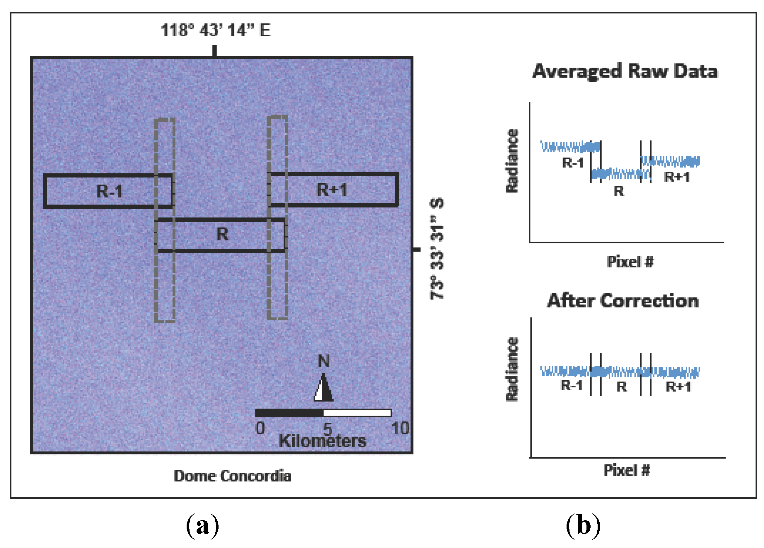
2.2. Enhanced Automated Processing: Finding Regions of Lowest Variability in Data

Previous work suggests a visual inspection to determine which region of the side slither data to use when deriving relative gains [2]. This section describes a simple methodology for identifying regions of lowest variability in the side slither data. By automatically identifying regions in the data that have minimal variability introduced by the scene, the derived relative gains can be calculated from data that reflect the instrument’s behavior, not in-scene (or human-induced) variability. This concept is illustrated with an example where the regions of minimal variability are identified in an actual TIRS side slither dataset.

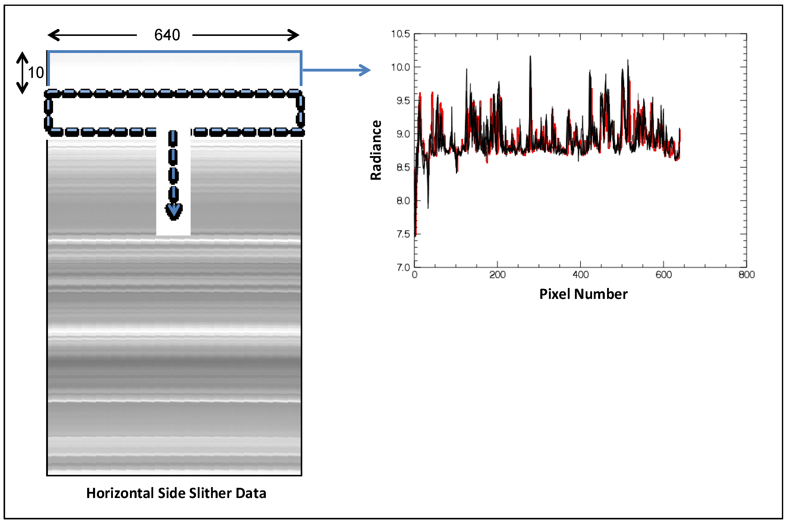
Figure 6 shows side slither data collected with SCA-A (sensor-chip assembly “A”) on the TIRS instrument after an enhanced horizontal correction has been applied. To determine regions of lowest scene-induced variability in this TIRS side slither data, the horizontal data of Figure 6 can be segmented into smaller regions and the variability calculated within each region. The TIRS sensor has 640 cross-track detectors in each array so the data was arbitrarily segmented into regions of size 10 × 640 for this study. The typical side slither collect contains several thousand frames (i.e., rows) of data so hundreds (perhaps thousands) of 10 × 640 regions may be characterized in this process.

To characterize the variability within each region, the column mean vector x is first calculated (red curve in Figure 6). Next, the deviations of each row vector from the column mean (black curves in Figure 6) are calculated and summed to describe the variability associated with the region. Finally, the region(s) with the minimum variability (or close to the minimum variability) can be used to calculate the relative gains, as these regions represent portions of the scene that introduce minimal in-scene variability. Mathematically, this concept is written.

$$min{\left({\sum }_{i=1}^{10}abs(x_i-\overline{x})\right)}_{j=1}^n$$

(7)

where i is the row number within a region, x_i is the ith row vector in a region, x is the mean column vector within a region, j is the region number, and n is the total number of regions being characterized. Qualitatively, regions where the radiance curves for each row vary the least from their corresponding column mean will be identified as low variability regions. Since several hundreds of regions will be characterized, the user can be selective as to how many regions to use in the final processing of relative gains. Once the regions are identified, the relative gains can be calculated in these regions according to Equation (5).

Figure 6. Illustration of automated processing method to find regions of lowest variability in the side slither data.

Figure 6. Illustration of automated processing method to find regions of lowest variability in the side slither data.

2.3. Site Identification

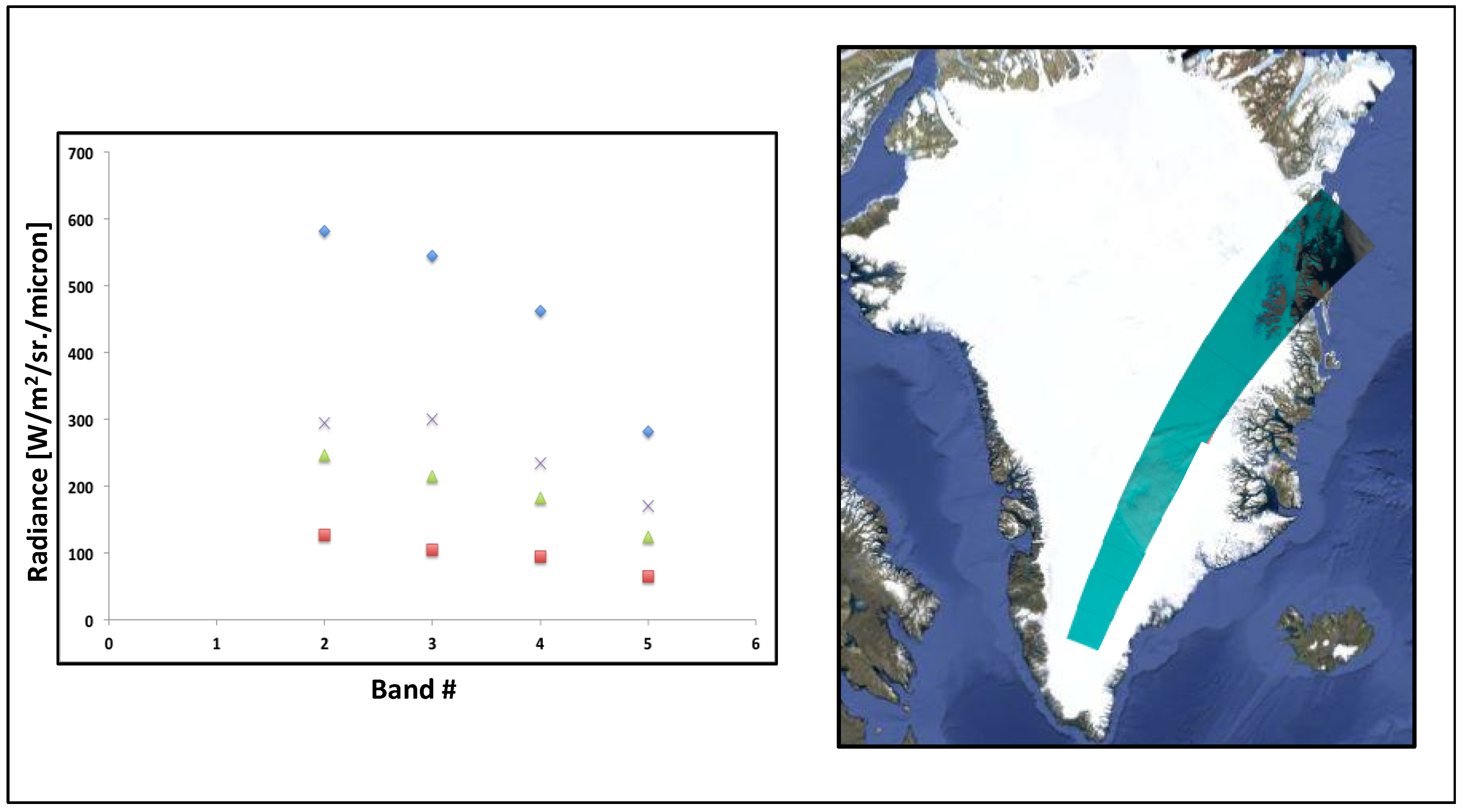
To determine worldwide sites that are favorable to support a side slither maneuver for Landsat 8, Gerace et al. 2012 [16] conducted a modeling effort focused on identifying uniform regions whose brightness values span the dynamic range of the OLI bands yet introduce minimal variability to the calculated relative gains. Sites of this nature are favorable for side slither as they can help identify potential detector nonlinearities while reducing pixel-to-pixel variability.

Basnet 2010 [17] conducted a statistical analysis with Landsat 5 data to identify potential worldwide pseudo-invariant calibration sites (PICS). Sites labeled as pseudo-invariant exhibited temporally and spatially stable brightness values in the data indicating that they were typically cloud free and that their landscape did not vary significantly. Sites of this nature are favorable for side slither missions as the potential risk of adverse weather is reduced in these regions. Gerace et al. 2012 [16] used these scenes for the side slither analysis by acquiring Landsat 5 images from Earth Explorer [18] and using their corresponding radiance data as input to the DIRSIG model.

For the initial modeling effort described in [16], a sensor model that did not include non-uniformity effects was developed to simulate the two center arrays of Landsat 8’s OLI sensor. Non-uniformity effects were excluded from this preliminary sensor model to determine the variability introduced by just the test site to properly assess its potential utility for side slither calibration. The sensor model was then used to image the Landsat radiance data in side slither mode and the variability in the corresponding relative gain coefficients was observed. 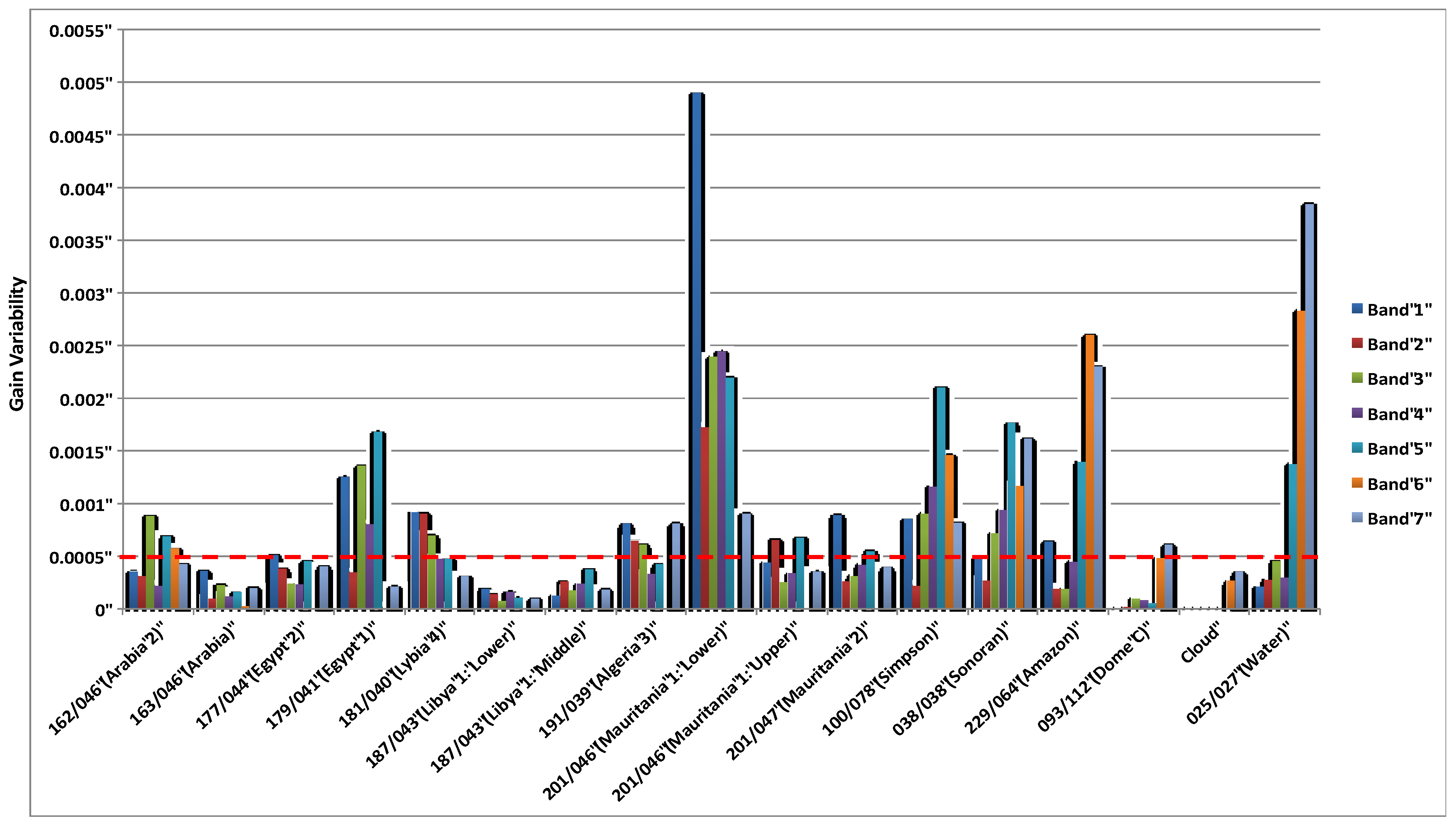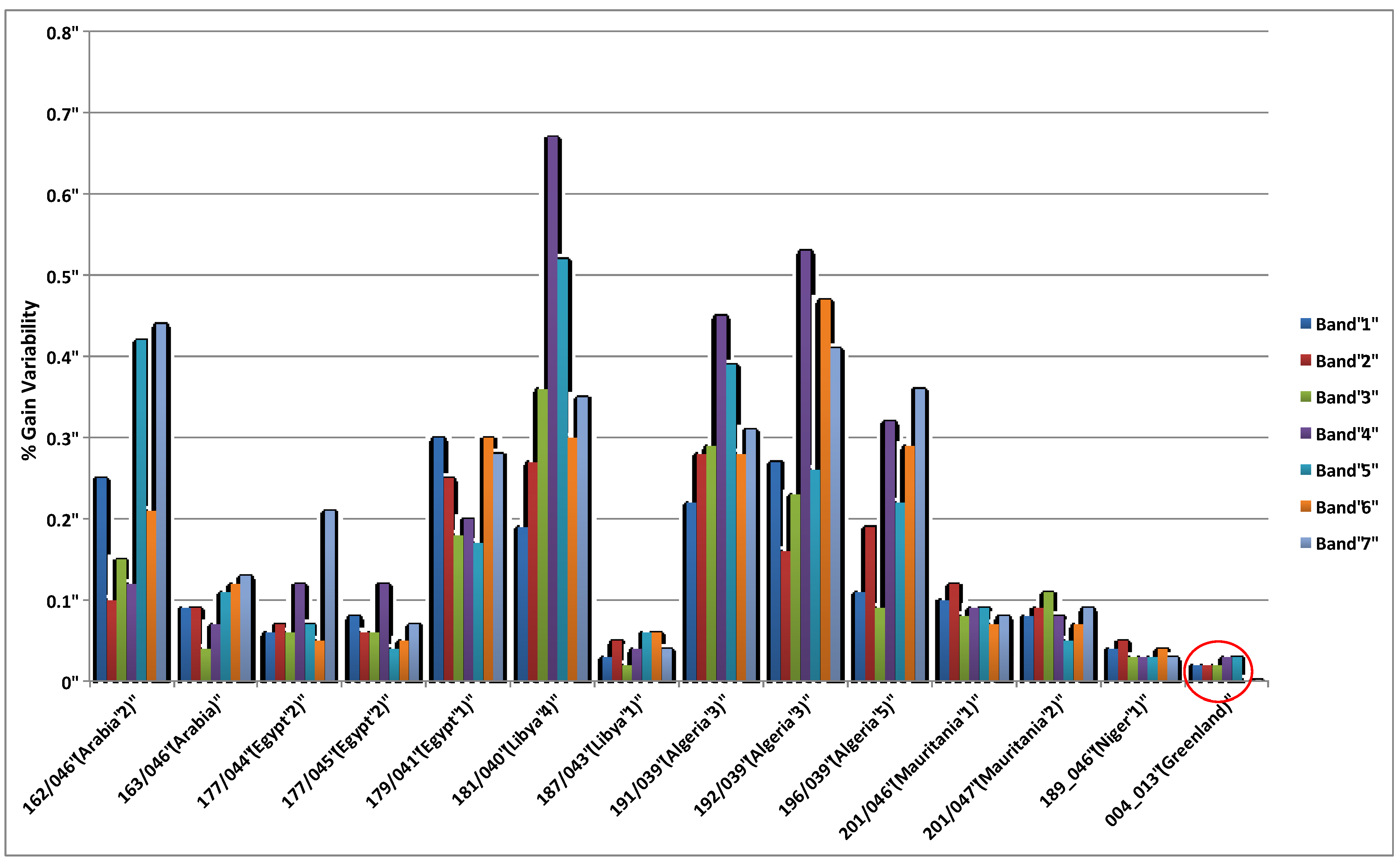Figure 7 shows the within-array variability introduced to the process by each of the sites with the maximum acceptable target error (0.05%) highlighted as a dashed (red) line. Note that this error target was chosen since it is an order of magnitude smaller than OLI’s pixel-to-pixel uniformity requirement (0.5%).

Figure 7. Within-array gain variability introduced by the sites listed in Table 1 for the first seven bands of the Operational Land Imager (OLI). The red dashed indicates the maximum acceptable target error of 0.0005 or 0.05%.

Figure 7. Within-array gain variability introduced by the sites listed in Table 1 for the first seven bands of the Operational Land Imager (OLI). The red dashed indicates the maximum acceptable target error of 0.0005 or 0.05%.

The variability described in Figure 7 represents the standard deviation divided by the mean of the relative gains (calculated using Equation (5)) within an array. Encouragingly, many of the sites studied in [16] introduce gain variability that is just at, or below, the threshold of 0.05% when the 2-array sensor model is used.

3. Significant Issues and Potential Solutions

3.1. Between-Array Variability

While the initial study of Section 2.3 helped identify potential sites to be used for the side slither maneuver, it also exposed an issue related to the calculation of relative gains. Figure 8a shows the relative gains calculated for Band 1 of OLI from the simulated side slither data imaged over the Dome Concordia dataset. A significant jump in relative gains occurs between the two arrays due to the ground track of the arrays during side slither mode.

Figure 8b shows the approximate ground-track for the two arrays when imaging in side-slither mode which, depending on the band, may be as much as 25 km apart. Over this distance, issues such as illumination gradients and BRDF effects due to the terrain and atmosphere can arise precluding the use of the side slither data to flat-field between arrays. Conveniently, to ensure data continuity, OLI has approximately 20 detectors of overlap between arrays in normal imaging mode that can be utilized to flat-field across arrays [7]. Although a full treatment of this process is beyond the scope of this article, Figure 9 briefly illustrates how the overlap detectors can be exploited in normal imaging mode to perform a relative calibration between arrays. Figure 9a illustrates three (of fourteen) arbitrary arrays from OLI and their corresponding overlap region when imaging in normal mode.

Figure 8. (a) Relative gains calculated for Band 1 of OLI from simulated side slither data collected over the Dome Concordia (b). Note that the ground track of the arrays has been plotted over the Dome Concordia RGB data to illustrate that the offset arrays image significantly different spots on the ground.

Figure 8. (a) Relative gains calculated for Band 1 of OLI from simulated side slither data collected over the Dome Concordia (b). Note that the ground track of the arrays has been plotted over the Dome Concordia RGB data to illustrate that the offset arrays image significantly different spots on the ground.

Figure 9. Illustration of how overlap region can be exploited to flat-field between arrays.

Figure 9. Illustration of how overlap region can be exploited to flat-field between arrays.

For this discussion, the middle array is labeled R, the left array R − 1, and the right array R + 1. To flat-field the data between arrays while imaging in normal mode (Figure 9a), several common in-track pixels (hundreds) imaged over a calibration site can be averaged for every detector in the overlap region to minimize temporal noise. The resulting averaged data is illustrated in Figure 9b(top). Then, to flatten the data between arrays, all detectors in an overlap region can be averaged and forced by ratio-ing to the average of the neighboring array’s overlap region, e.g., Figure 9b(bottom) illustrates how the average of the detectors in the overlap region of the R − 1 and R + 1 arrays can be forced to agree with averaged overlap values in array R.

3.2. “Smearing” in Edge Arrays

Section 2.3 identified calibration sites that are suitable for the side slither maneuver. While several sites are identified as favorable, the analysis was conducted with only the two center arrays of OLI. When projected through the optics, the edge arrays of OLI appear skewed approximately one degree from the center arrays. This can potentially impact the flat-fielding process when using relative gains calculated from the side slither maneuver, as the edge arrays will not experience a perfect 90-degree yaw.

To validate the hypothesis that features in the landscape may introduce significantly higher gain variability in the edge arrays of OLI, a large-scale synthetic landscape of the Libya 4 PICS was developed with a single material type (sand) and used as input to DIRSIG, see Figure 10. This site has traditionally been used for Landsat calibration [19] and remains ideal for long-term drift analysis. However, Libya 4 exhibits features (e.g., sand dunes) that diminish its utility of side slither data. The projection of the OLI arrays is overlaid to illustrate the difference in orientation between the edge arrays and the middle arrays in side slither mode. The middle arrays (red oval) used in the preliminary study of Section 2.3 are parallel to the ground-track when in side slither mode while the edge arrays (e.g., blue circle) are not. When features exist in the landscape (e.g., a sand dune as shown by the blue arrow), each detector of the array will image a slightly different portion of the feature leading to an undesirable “smearing” in the side slither data.

Side slither simulations were performed over the synthetic Libya 4 landscape shown in Figure 10 using a DIRSIG sensor model developed from the line-of-site (LOS) vectors for all 14 OLI arrays. Note that only OLI band 1 was modeled for this study but all sources of non-uniformity (i.e., detector-to-detector gains, biases, relative spectral response functions, noise, and quantization) were incorporated. The resulting data after performing a horizontal correction is shown in Figure 11(top).

Notice that the data for several arrays (blue circles) exhibit “smearing” due to the orientation of these arrays as they image over non-uniform features in the landscape in side slither mode. Using this data for calibration will introduce significant variability into the final data product. To quantify the magnitude of the variability introduced by smearing in the edge arrays, a flat plate of sand (the same sand used in the Libya 4 scene shown in Figure 10) was developed and provided as the scene input to DIRSIG. The same Band 1 sensor model that was used to generate the side slither data in Figure 11(top) was used to image the flat plate in normal imaging mode. The side slither data of Figure 11(top) was then used to perform an array-by-array relative calibration on the flat plate data. The desired result of this calibration process is a uniform brightness across the entire flat plate.

Figure 10. Synthetic Libya 4 landscape developed to illustrate the impact of in-scene variability on side slither relative calibration process. The red oval highlights the 2 center arrays of OLI. The blue circle highlights an edge array and its orientation with respect to significant features in the landscape when imaging in side slither mode.

Figure 10. Synthetic Libya 4 landscape developed to illustrate the impact of in-scene variability on side slither relative calibration process. The red oval highlights the 2 center arrays of OLI. The blue circle highlights an edge array and its orientation with respect to significant features in the landscape when imaging in side slither mode.

Figure 11. Top frame shows the resulting side slither data (after a horizontal correction has been applied) when imaging over the Libya 4 simulated landscape with all 14 arrays of OLI. The bottom frame shows the result of applying a side slither correction to a flat plate of sand with the relative gains obtained from the top frame. The blue circles highlight the smearing effect caused by arrays that are not oriented at 90 degrees when in side slither mode.

Figure 11. Top frame shows the resulting side slither data (after a horizontal correction has been applied) when imaging over the Libya 4 simulated landscape with all 14 arrays of OLI. The bottom frame shows the result of applying a side slither correction to a flat plate of sand with the relative gains obtained from the top frame. The blue circles highlight the smearing effect caused by arrays that are not oriented at 90 degrees when in side slither mode.

Figure 11(bottom) shows that instead of obtaining a uniform image, as would be expected when flat-fielding a uniform scene, the correction process actually introduced significant striping and banding to the calibrated image data. The banding and striping is not significant in the middle arrays but becomes increasingly significant toward the edge arrays indicating that the terrain-induced smearing is a function of the array orientation when imaging with a 90-degree yaw.

By using the processing method described in Section 2.2 and choosing scenes with minimal terrain features (e.g., Dome C, Greenland, Niger, Mauritania, Saudi Arabia) as described in Section 2.3 & Section 3.3, the impact of terrain-induced smearing can be minimized. For satellite systems versatile enough to perform side slither in the first place, an alternative methodology that can further reduce smearing in the edge arrays is now introduced.

Figure 12 shows the column average DN as a function of detector number for the “calibrated” data shown in Figure 11(bottom). While the variability across the full field-of-view is approximately 4.5%, the variability within the center 2000 detectors is less than 0.5%. Recall, from Figure 10 (red circle), that the center arrays in the nominal side slither maneuver are parallel to the direction of motion so low variability is expected in this region.

Figure 12. Column average of the mis-calibrated data shown in Figure 11(bottom). Note that although variability across the entire field-of-view is in excess of 4.5%, the variability in the center region (between blue lines) is less than 0.5%.

Figure 12. Column average of the mis-calibrated data shown in Figure 11(bottom). Note that although variability across the entire field-of-view is in excess of 4.5%, the variability in the center region (between blue lines) is less than 0.5%.

To reduce the variability due to smearing in the edge arrays, additional side slither maneuvers can be performed over a site to align the edge arrays with the direction of motion. To test this hypothesis, two side slither maneuvers in addition to the nominal 90-degree maneuver were simulated in DIRSIG over the Libya 4 synthetic landscape and the corresponding relative gains used to correct the flat plate of sand. One maneuver was conducted at 89 degrees to align the port side arrays and the other at 91 degrees to align the starboard side arrays to the direction of motion. Figure 13 shows the column-averaged results of the corrected flat plate image and illustrates the potential effectiveness of this procedure.

Figure 13(left) shows a significant reduction in variability in the first 4000 detectors (StdDev/Mean = 0.7%) while Figure 13(right) shows a significant reduction in variability in the last 3000 detectors (StdDev/Mean = 0.9%). When combined with the nominal 90-degree maneuver, the variability across the full FOV can be reduced from 4.5% to under 0.9% in this case.

Figure 13. Column averages of calibrated side slither data resulting from maneuvers of (a) 89 degrees and (b) 91 degrees respectively.

Figure 13. Column averages of calibrated side slither data resulting from maneuvers of (a) 89 degrees and (b) 91 degrees respectively.

3.3. Revisiting Site Identification

To build on the work of Section 2.3, an additional study was conducted to identify potential sites for the side slither maneuver. This subject was revisited for several reasons but primarily to determine the variability introduced by potential sites when the full FOV of OLI was considered and to incorporate additional sites that would be suitable for the commissioning phase of LDCM. Due to its February launch, the Dome Concordia site, which exhibits extremely low variability (see Figure 7), would not have the proper illumination for calibration once LDCM achieved its final orbit. Anderson et al. 2011 [2] demonstrated success with the Greenland site so an additional investigation was conducted to determine if this site was suitable for the Landsat 8 instruments.

3.3.1. Greenland

Greenland exhibits several regions of low variability that indicate that it may be suitable for the side slither maneuver. The traditional calibration sites from Section 2.3 that are used for long-term drift analysis typically span a fraction of a path/row on the World Reference System 2 (WRS2). Greenland, on the other hand, spans several (>10) path/rows. This is preferable for side slither maneuvers as it increases the likelihood of imaging a uniform region.

Perhaps even more intriguing is the wide range of illumination conditions that it experiences throughout the year. Figure 14(left) shows the minimum (red squares) and the maximum (green triangles) radiance levels (W/m²/sr/micron) for the VNIR bands of Landsat 7 that were observed in the over-flight data shown in Figure 14(right). These Landsat 7 data, which were used as input to DIRSIG to test the variability introduced by the site, were collected close to the equinox. Interestingly, Landsat 7 data for the months between April and August were also tested but the data were saturated even though ETM+ is set to its low gain setting over Greenland for these months [20]. The purple x’s of Figure 14 show the saturation radiances for Landsat 7 while the blue diamonds show the saturation radiances for Landsat 8. These data indicate that Greenland is suitable for characterizing potential nonlinearities in the lower to middle regions (and perhaps the middle to higher end) of OLI’s dynamic range.

Due to its location with respect to Landsat’s orbit, a side slither can be performed over Greenland with minimal loss of land imaging for the rest of the path. As is the case with any other site with snow, Greenland is not suitable for calibrating SWIR bands, as snow appears dark in the shortwave infrared. However, the potential upsides to this site warranted further analysis.

Figure 14. Figure illustrating a swath over Greenland (right) that is suitable for the side slither maneuver and the corresponding radiance levels observed in Landsat image data. The red squares show the minimum radiance levels and the green triangles show the maximum radiance levels observed in the Greenland test data. The purple x’s show the saturation levels for ETM+ while the blue diamonds show the saturation levels for OLI.

Figure 14. Figure illustrating a swath over Greenland (right) that is suitable for the side slither maneuver and the corresponding radiance levels observed in Landsat image data. The red squares show the minimum radiance levels and the green triangles show the maximum radiance levels observed in the Greenland test data. The purple x’s show the saturation levels for ETM+ while the blue diamonds show the saturation levels for OLI.

3.3.2. Niger and a Qualitative Characterization of Suitable Sites

A second site that was included in this additional analysis was the Niger site located at path 189, row 046 in the WRS2. This site was included due to its apparent low spatial variability and infrequent cloud cover. The inclusion of this site, which does not show up as a PICS in the Earth Explorer data, raises the question, “What spatial characteristics make a site suitable for the side slither maneuver?” While a full analysis of this matter was not investigated, Figure 15 offers a qualitative (yet intuitively satisfying) explanation.

The four true-color images in Figure 15a show the center 30 km for four PICS used in the preliminary side slither analysis of Section 2.3. These data are grouped together as they represent the sites that introduce the most gain variability in the side slither study. While these sites have been historically, and continue to be, suitable for long-term drift analysis due to their invariant nature, they introduce excessive gain variability to be used for side slither calibration with instruments exhibiting a wide in-track FOV. Recalling the discussion of Section 3.2, the sites of Figure 15a all contain significant features in the terrain throughout the landscape that will significantly impact gain variability.

Figure 15. A visual comparison of the potential side slither sites tested in this work. (a) shows the sites that introduce the most error to the side slither-derived relative gains, (b) shows sites that introduce an acceptable error, and (c) shows the sites that introduce the least error. Note that sites whose image data resemble system noise introduce insignificant error to the process indicating that land features have minimal impact on the sensor-reaching signal. (d) shows additional side slither test sites that were chosen based on their visual appearance.

Figure 15. A visual comparison of the potential side slither sites tested in this work. (a) shows the sites that introduce the most error to the side slither-derived relative gains, (b) shows sites that introduce an acceptable error, and (c) shows the sites that introduce the least error. Note that sites whose image data resemble system noise introduce insignificant error to the process indicating that land features have minimal impact on the sensor-reaching signal. (d) shows additional side slither test sites that were chosen based on their visual appearance.

Figure 15b shows sites that introduced acceptable gain variability to the side slither process. While significant features exist in the landscape for these PICS, there are also regions (highlighted by the red boxes) that exhibit low spatial variability. The automated process of Section 2.2 finds these low variability regions and includes them in the relative gain calculation.

The two images in Figure 15c show sites from Figure 7 that introduce the least variability. The zoom windows show that Libya 1 and the Dome C both contain large regions where the landscape resembles system noise. This indicates that the variability in the landscape is not significant enough to impact the sensor-reaching signal. Sites of this nature are desirable for the side slither maneuver when using a sensor with a wide in-track FOV. Finally, Figure 15d shows a small portion of the Greenland and Niger test sites. As shown in the zoom windows, they also exhibit regions that resemble system noise, indicating that they will likely introduce variability that is in-line with Libya 1 and the Dome C.

Although this discussion characterizes uniform sites qualitatively, the methods described by Hu et al. 2012 [21] to characterize system noise can be applied directly to develop a quantitative characterization of sites suitable for side slither. A qualitative characterization of the sites could potentially take the place of the extensive analysis described in Section 2.3 and the next section.

3.3.3. Site Identification Incorporating OLI’s Full FOV

The experiment described in Section 2.3 was repeated but with the additional sites included and with OLI’s full FOV incorporated, i.e., Section 2.3 used the center 2 arrays for the sensor model whereas this study incorporated all 14 arrays in the sensor model. Landsat 5 radiance data was used as input to DIRSIG for all sites save Greenland where Landsat 7 data was used. The results of the gain variability introduced by all sites are shown in Figure 16. As expected, Niger, Greenland, and Libya 1 introduce the least variability to the relative gains (Note that although Greenland replaced the Dome C in this study, the Dome C is the preferred snow site due to its high elevation, small change in elevation, and favorable weather conditions [17].

The results shown in Figure 16 further verify that visual inspection or a simple statistical analysis [21] can be used to identify sites suitable for the side slither maneuver (as opposed to the significant modeling effort performed in this work). As hypothesized in Figure 15d, both Niger and Greenland introduce negligible variability to the side slither-derived relative gains. Figure 16 indicates that several sites are suitable for the side slither maneuver if the data are processed carefully.

3.4. Using Side Slither to Potentially Identify Stray Light

Early on in the mission, there was convincing evidence that Landsat 8’s thermal instrument TIRS had a stray light issue. Significant effort has been, and continues to be, made to identify and remove stray light from TIRS image data, see [22] for a full treatment. An interesting find was made during the processing of TIRS side slither data collected over the Mediterranean that supports the presence of stray light.

Figure 16. Results showing the side slither-derived gain variability for several of the original sites included in Section 2.3 and the additional Niger and Greenland sites. Note that the study in Section 2.3 used only the center 2 arrays for the sensor model while this study incorporated all 14 arrays into its sensor model.

Figure 16. Results showing the side slither-derived gain variability for several of the original sites included in Section 2.3 and the additional Niger and Greenland sites. Note that the study in Section 2.3 used only the center 2 arrays for the sensor model while this study incorporated all 14 arrays into its sensor model.

Figure 17 shows horizontally corrected Band 11 TIRS side slither data collected from SCA-A (left) and SCA-B (center). These two arrays image nearly the same ground-track in side slither mode so the images should appear the same other than non-uniformity effects in the instrument. When the two images are differenced, however, artifacts due to stray light are present.

Figure 17(right) shows the resulting image when the two datasets are differenced (A-B). As expected, residual striping is apparent due to differing non-uniformity effects in the two arrays. Also, the white stripe highlighted by the purple rectangle is a landmass (Cyprus). This landmass is appropriately absent in the difference image. The orange circles, however, highlight stray light captured by SCA-B as TIRS approaches Cyprus (top circle) and Egypt (bottom circle) in side slither mode. Montanaro et al. 2014 [22] confirm that the source of the stray light for SCA-B would be over land when the stray light appears in the orange circles of Figure 17(right).

This find is somewhat discouraging in that it currently precludes TIRS side slither data from being used to flat-field image data without first applying a stray light preprocessing step. However, there may be some value in this data in that it potentially lends insight into the magnitude of the stray light on a per-detector basis since each detector should theoretically image the same spot on the ground. Using side slither data to derive the magnitude of stray light remains an area of ongoing research.

Figure 17. Artifacts due to stray light are present in TIRS band 11 side slither image data. (Left) shows horizontally corrected SCA-A side slither data, (middle) shows horizontally corrected SCA-B side slither data, and (right) shows the difference image. Significant artifacts exist in the orange circles indicating the presence of stray light. The purple square highlights a landmass (Cyprus) which is appropriately removed in the difference image (right).

Figure 17. Artifacts due to stray light are present in TIRS band 11 side slither image data. (Left) shows horizontally corrected SCA-A side slither data, (middle) shows horizontally corrected SCA-B side slither data, and (right) shows the difference image. Significant artifacts exist in the orange circles indicating the presence of stray light. The purple square highlights a landmass (Cyprus) which is appropriately removed in the difference image (right).

4. Conclusions, Future Work, and Recommendations

While previous work [1,2] demonstrates the potential to use side slither to flat-field image data for sensors with a narrow field-of-view, this work uses simulation and modeling to investigate potential issues with the maneuver when applied to sensors (such as those onboard Landsat 8) with a wide field-of-view. The modeling efforts performed in this work led to several significant conclusions.

Section 2.1 shows a proper horizontal correction should be applied to avoid introducing low-frequency artifacts into the corrected image data. In Section 2.2, an automated processing technique designed to find region(s) of lowest variability in the side slither data was introduced. This simple method was devised to ensure that the most uniform regions in the data were being used to derive relative gains. Section 2.3 and Section 3.3 described a methodology that was conceived to identify and characterize sites around the globe that may be suitable for the side slither maneuver.

In Section 3, potential issues that may arise when imaging in side slither mode were presented. The most notable and most likely to negatively impact the data is the concept of “smearing”, which occurs when arrays are not aligned exactly 90 degrees to significant features in the landscape. There are two methods to avoid this unwanted effect; avoid any features by choosing the most uniform regions on Earth (see Figure 16) or performing multiple side slithers over a chosen region to align all the arrays properly. Failure to employ one of these methods will likely lead to banding in the corrected image data, recall Figure 11(bottom).

Future modeling efforts to characterize the utility of the calibration sites presented here for side slither calibration will focus on the incorporation of BRDF effects. All studies performed in this work used existing Landsat data or simulated data with Lambertian materials (e.g., the Libya 4 scene in Figure 10). Although the effects due to the terrain (and in some cases the relevant atmospheric paths) were present in the simulations performed in this work, the impact of material BRDFs on side slither calibration was not conducted. Recent enhancements to the DIRSIG model, however, have made the incorporation of BRDF effects possible for the large-scale landscapes required for a comprehensive analysis of the side slither maneuver.

Much of the work presented here has been recommended to, and employed by, the Landsat Calibration and Validation team. Several side slither maneuvers were conducted during the commissioning phase of Landsat 8, including successful maneuvers over Niger and Greenland. The side slither maneuver continues to be part of normal operations where once a quarter, the maneuver is performed over the most suitable available sites from Figure 16.

References

1. Henderson, B.G.; Krause, K.S. Relative radiometric correction of QuickBird imagery using the side-slither technique on-orbit. Proc. SPIE 2004, 5542, 426–436. [Google Scholar]
2. Anderson, C.; Naughton, D.; Brunn, A.; Thiele, M. Radiometric correction of RapidEye imagery using the on-orbit side-slither method. Proc. SPIE 2011, 8180, 1–15. [Google Scholar]
3. Xiong, X.; Barnes, W. An overview of MODIS radiometric calibration and characterization. Adv. Atmos. Sci. 2006, 23, 69–79. [Google Scholar]
4. Mika, A.M. Three decades of Landsat instruments. Photogramm. Eng. Remote Sens. 1997, 63, 839–852. [Google Scholar]
5. Markham, B.L.; Barker, J.L.; Barsi, J.A.; Kaita, E.; Thome, K.J.; Helder, D.L.; Palluconi, F.D.; Schott, J.R.; Scaramuzza, P. Landsat-7 ETM+ radiometric stability and absolute calibration. Proc. SPIE 2003, 4881, 308–318. [Google Scholar]
6. Schott, J.R. Imaging sensors and instrument calibration. In Remote Sensing: The Image Chain Approach, 2nd ed.; Oxford University Press: New York, NY, USA, 2007; pp. 207–208. [Google Scholar]
7. Knight, E.; Kvaran, G. Landsat-8 Operational Land Imager design, characterization, and performance. Remote Sens. 2014, 6, 10286–10305. [Google Scholar]
8. Markham, B.L.; Barsi, J.A.; Kvaran, G.; Ong, L.; Kaita, E.; Biggar, S.; Czapla-Myers, J.; Mishra, N.; Helder, D.L. Landsat-8 Operational Land Imager radiometric calibration and stability. Remote Sens. 2014, in press. [Google Scholar]
9. Reuter, D. The Thermal Infrared Sensor (TIRS) on Landsat 8: Design overview and pre-launch characterization. Remote Sens. 2014, in press. [Google Scholar]
10. Xiong, X.; Erives, H.; Xiong, S.; Xie, X.; Esposito, J.; Sun, J.; Barnes, W. Performance of Terra MODIS solar diffuser and solar diffuser stability monitor. Proc. SPIE 2005, 5882. [Google Scholar] [CrossRef]
11. Schott, J.R.; Brown, S.D.; Raqueno, R.V.; Gross, H.N.; Robinson, G. An advanced synthetic image generation model and its application to multi/hyperspectral algorithm development. Can. J. Remote Sens. 1999, 25, 99–111. [Google Scholar]
12. Brown, S.D.; Sanders, N.J.; Goodenough, A.A.; Gartley, M. Modeling space-based multispectral imaging systems with DIRSIG. Proc. SPIE 2011, 8048. [Google Scholar] [CrossRef]
13. Schott, J.R.; Gerace, A.D.; Brown, S.D.; Gartley, M.G. Modeling the image performance of the Landsat Data Continuity Mission sensors. Proc. SPIE 2011, 8153. [Google Scholar] [CrossRef]
14. Gerace, A.; Gartley, M.; Schott, J.; Raqueno, N.; Raqueno, R. Data-driven simulations of the Landsat Data Continuity Mission (LDCM) platform. Proc. SPIE 2011. [Google Scholar] [CrossRef]
15. Schott, J.; Gerace, A.; Brown, S.; Gartley, M.; Montanaro, M.; Reuter, D.C. Simulation of image performance characteristics of the Landsat Data Continuity Mission (LDCM) Thermal Infrared Sensor (TIRS). Remote Sens. 2012, 4, 2477–2491. [Google Scholar]
16. Gerace, A.D.; Schott, J.R.; Brown, S.D.; Gartley, M.G. Using DIRSIG to identify uniform sites and demonstrate the utility of the side-slither calibration technique for Landsat’s new pushbroom instruments. Proc. SPIE 2012, 8390. [Google Scholar] [CrossRef]
17. Basnet, B. Identification of Worldwide Optimal Pseudo-Invariant Calibration Sites for Post-Launch Radiometric Calibration of Earth Observation Satellite Sensors. Master’s Thesis, South Dakota State University, Brookings, SD, USA, 2010. [Google Scholar]
18. EarthExplorer. Available online: http://earthexplorer.usgs.gov (accessed on 1 January 2014).
19. Markham, B.L.; Barsi, J.A.; Helder, D.L.; Thome, K.T.; Barker, J.L. Evaluation of the Landsat-5 TM radiometric calibration history using desert test sites. Proc. SPIE 2006, 6361. [Google Scholar] [CrossRef]
20. NASA Goddard Space Flight Center (GSFC). Landsat 7 Science Data Users Handbook. Available online: http://landsathandbook.gsfc.nasa.gov/data_properties/prog_sect6_4.html (accessed on 1 January 2014).
21. Hu, C.; Feng, L.; Lee, X.; Davis, C.O.; Mannino, A.; McClain, C.R.; Franz, B.A. Dynamic range and sensitivity requirements of satellite ocean color sensors: Learning from the past. Appl. Opt. 2012, 51, 6045–6062. [Google Scholar]
22. Montanaro, M.; Gerace, A.; Lunsford, A.; Reuter, D. Stray light artifacts in imagery from the Landsat 8 thermal infrared sensor. Remote Sens. 2014, 6, 10435–10456. [Google Scholar]