Landsat 8 Operational Land Imager On-Orbit Geometric Calibration and Performance

Abstract

The Landsat 8 spacecraft was launched on 11 February 2013 carrying the Operational Land Imager (OLI) payload for moderate resolution imaging in the visible, near infrared (NIR), and short-wave infrared (SWIR) spectral bands. During the 90-day commissioning period following launch, several on-orbit geometric calibration activities were performed to refine the prelaunch calibration parameters. The results of these calibration activities were subsequently used to measure geometric performance characteristics in order to verify the OLI geometric requirements. Three types of geometric calibrations were performed including: (1) updating the OLI-to-spacecraft alignment knowledge; (2) refining the alignment of the sub-images from the multiple OLI sensor chips; and (3) refining the alignment of the OLI spectral bands. The aspects of geometric performance that were measured and verified included: (1) geolocation accuracy with terrain correction, but without ground control (L1Gt); (2) Level 1 product accuracy with terrain correction and ground control (L1T); (3) band-to-band registration accuracy; and (4) multi-temporal image-to-image registration accuracy. Using the results of the on-orbit calibration update, all aspects of geometric performance were shown to meet or exceed system requirements.

1. Introduction and Overview

The Landsat 8 Operational Land Imager (OLI) is a push-broom (linear array) imaging system that collects visible, NIR, and SWIR spectral band imagery at 30-meter (15-meter panchromatic) ground sample distance [1]. By collecting a 190-kilometer-wide image swath from a 705-kilometer orbital altitude, the OLI provides continuity with the heritage whisk-broom (cross-track scanning mirror) architecture Thematic Mapper (TM) and Enhanced Thematic Mapper Plus (ETM+) sensors flown on Landsats 4, 5, and 7. The OLI’s push-broom architecture [2] led to some differences in the geometric modeling and calibration approach used for Landsat 8 as compared to the previous systems. At a high level, these differences involve ensuring the proper alignment of all focal plane elements across the full instrument field of view rather than characterizing the dynamics of a scanning mirror subsystem. This paper describes the geometric calibration operations that were performed to refine the OLI geometric model during the 90-day commissioning period following the 11 February 2013 launch, and then presents the geometric performance of the operational OLI image products with respect to geolocation accuracy, band registration accuracy, and image registration accuracy utilizing the results of the on-orbit calibration activity.

The remainder of this section describes the objectives of the on-orbit geometric calibration exercise in more detail, presents the approach adopted to accomplish those objectives, and defines in more detail the key geometric performance characteristics that were measured and verified on-orbit. The second section of the paper provides an overview of the OLI prelaunch geometric calibration and then describes the details of the on-orbit geometric calibration campaign. The third section presents the geometric performance results that were observed following the on-orbit calibration activities. The final sections summarize the current state of Landsat 8 OLI geometric calibration and performance and provide a brief description of one way the excellent geometric performance achieved by Landsat 8 is being used to improve the accuracy of the global ground control point network that is used to register all Landsat data products to the Global Land Survey (GLS) geometric framework.

1.1. Geometric Calibration Approach

The fundamental objective of geometric calibration is to provide line-of-sight direction/angles for each active detector relative to the spacecraft attitude control system reference frame, to support accurate image geolocation. The parameters of the geometric line-of-sight model are refined through the geometric calibration process to suppress systematic errors that degrade detector pointing knowledge and the resulting geolocation accuracy. The geometric characterization obtained by monitoring geometric performance during routine imaging operations provide the data required to adjust the geometric calibration as necessary to maintain geometric accuracy. Viewed as a process of tuning the geometric line-of-sight model to achieve the desired geometric performance, the details of geometric calibration can be seen to be dependent upon the geometric model formulation.

The initial OLI geometric line-of-sight model was derived based upon the sensor design, prior to the fabrication of any OLI hardware components. The OLI design is described in Knight et al. [2], but a few key aspects of the design are worth repeating here. In particular, the OLI focal plane layout, shown in Figure 1, strongly influenced the organization of the geometric model and the associated calibration parameters and methods.

Figure 1. The Operational Land Imager (OLI) focal plane layout showing: top—the arrangement of the visible and near infrared (VNIR) and short-wave infrared (SWIR) spectral bands in the along-track direction; and bottom—the 14 focal plane modules across the OLI field of view.

Figure 1. The Operational Land Imager (OLI) focal plane layout showing: top—the arrangement of the visible and near infrared (VNIR) and short-wave infrared (SWIR) spectral bands in the along-track direction; and bottom—the 14 focal plane modules across the OLI field of view.

The OLI detectors are distributed across 14 separate focal plane modules (FPMs), each of which covers a portion of the 15-degree OLI cross-track field of view. Adjacent FPMs are offset in the along-track direction to allow for FPM-to-FPM overlap, avoiding any gaps in the cross-track coverage. Each FPM contains detectors and associated filters for each of the nine OLI spectral bands, plus a dark band used for radiometric calibration. The internal layout of all 14 FPMs is the same, with alternate FPMs being rotated by 180-degrees to keep the active detector areas as close together as possible. This has the effect of inverting the along-track order of the spectral bands in adjacent FPMs. The OLI can be thought of as being composed of 14 individual sub-sensors, each of which covers approximately 1/14th of the cross-track field of view. Knowledge of the precise placement and orientation of each FPM is crucial for achieving an accurate geometric calibration of the OLI.

The initial prelaunch geometric model was constructed by calculating the locations of each detector on the OLI focal plane, based upon the nominal placement of each FPM, and then projecting these detector locations through the OLI optics into object space using the design parameters of the OLI telescope. This provided nominal viewing vectors and associated angles for each detector based upon the nominal focal plane layout and telescope optical performance. The resulting nominal design geometric model was used for algorithm development and data simulation while the OLI instrument was being assembled. A plot showing the line-of-sight angles for the end points and center of each band on each FPM is shown in Figure 2. Note that the vertical scale is exaggerated by a factor of approximately 8 in the figure to make the spectral band ordering easier to visualize. Also note the slight rotation of the FPMs away from the center of the field of view. This rotation was introduced intentionally to compensate for optical distortion.

Figure 2. The OLI line-of-sight pattern with the along-track scale, exaggerated by a factor of ~8 to highlight the off-nadir focal plane module (FPM) rotation intended to compensate for optical distortion.

Figure 2. The OLI line-of-sight pattern with the along-track scale, exaggerated by a factor of ~8 to highlight the off-nadir focal plane module (FPM) rotation intended to compensate for optical distortion.

During OLI prelaunch testing the nominal geometric model was refined using line-of-sight direction measurements for selected detectors. These measurements were collected by scanning small horizontal and vertical slit targets across a few detectors in each FPM during instrument-level thermal vacuum testing [2]. These measurements were used to correct the nominal FPM location and orientation parameters and to refine the telescope optical parameters. The refined parameters were then used to create a new set of detector lines-of-sight, which formed the basis of the prelaunch geometric model.

Following launch, instrument activation, and initial check-out, OLI images processed using the prelaunch geometric model were analyzed using ground control point measurements, reference images, and band-to-band comparisons. These measurements and the associated analyses, described below, were used to perform the on-orbit refinement of the geometric model and to create the operational set of geometric calibration parameters. Each of these iterations of model refinement: design, prelaunch, and on-orbit; produced a set of geometric model calibration parameters, stored in a Calibration Parameter File (CPF). This file packages the static, or slowly varying (e.g., sensor alignments that may vary seasonally), elements of the geometric model in a single place to simplify their application during product generation. A new CPF is typically generated every calendar quarter to refresh the continuously changing Earth orientation parameters. More frequent updates are issued if needed to compensate for observed changes in on-orbit behavior.

1.2. Key Geometric Performance Characteristics

OLI geometric performance was specified and is now measured with respect to four key characteristics [3]. These characteristics and the required performance levels for both Landsat 8 and Landsat 7 [4] are shown in Table 1.

Table 1. Landsat 7 ETM+ and Landsat 8 OLI geometric performance requirements.

Requirement	ETM+ Specification	ETM+ Performance	OLI Specification
Absolute Geodetic Accuracy (CE90)	536.5 meters	45–190 meters (varied with gyro health)	65 meters
Geometric (Terrain Corrected) Accuracy (CE90)	N/A	15 meters	12 meters
Band Registration Accuracy (LE90)	8.4 meters	3.0 meters (reflective bands)	4.5 meters
Image Registration Accuracy (LE90)	12.0 meters	10.5 meters	12 meters

Table 1. Landsat 7 ETM+ and Landsat 8 OLI geometric performance requirements.

Requirement	ETM+ Specification	ETM+ Performance	OLI Specification
Absolute Geodetic Accuracy (CE90)	536.5 meters	45–190 meters (varied with gyro health)	65 meters
Geometric (Terrain Corrected) Accuracy (CE90)	N/A	15 meters	12 meters
Band Registration Accuracy (LE90)	8.4 meters	3.0 meters (reflective bands)	4.5 meters
Image Registration Accuracy (LE90)	12.0 meters	10.5 meters	12 meters

Absolute geodetic accuracy refers to the geolocation accuracy of geometrically corrected products prior to the application of ground control points. The geolocation accuracy achieved is primarily dependent upon spacecraft performance (e.g., attitude and ephemeris knowledge) but also involves OLI instrument pointing knowledge and stability. The geometric calibration parameter most relevant to achieving the required geolocation accuracy is the alignment knowledge between the OLI and the spacecraft attitude control system. The required accuracy of 65 meters 90% circular error (CE90) was selected to ensure Landsat 8 accuracy commensurate with the accuracy achieved by Landsat 7 prior to the degradation of that system’s inertial reference units (gyroscopes). Although both Landsat 7 and Landsat 8 data products are corrected using ground control points derived from the Global Land Survey (GLS) image data set, having accurate a priori image location knowledge makes the control point matching process more reliable, particularly in partially cloud-covered images.

The accuracy of the final OLI Level 1T radiometrically- and geometrically-corrected data product, including the application of ground control point and digital terrain model corrections, is referred to as geometric accuracy. The absolute accuracy of a ground control corrected product is dependent upon the accuracy of the control itself, so this specification explicitly assumed that ground control points accurate to 3 meters (CE90) horizontally and 12 meters 90% linear error (LE90) vertically were available for use in both geometric correction and accuracy verification [3]. Geometric accuracy is measured at characterization sites where highly accurate ground control points are available but the GLS-derived control points used for operational product generation do not generally conform to this level of accuracy. Practical Level 1T product accuracy is therefore the combination of the Landsat 8 system geometric accuracy and the inherent accuracy of the GLS ground control framework (nominally 25 meters root-mean-square-radial) [5].

The OLI band-to-band registration accuracy specification defines the accuracy with which corresponding Level 1T product pixels from different OLI spectral bands must be co-aligned. It is important to note that this requirement applies to Level 1T products, that is, after geometric correction including image resampling. The OLI sensor architecture does not provide inherent registration between spectral bands as the data are collected. The detectors for each spectral band are aligned in parallel rows distributed along-track as shown in Figure 2. The spectral bands thus image a given ground target at slightly different times as the detector array is “pushed” across the ground by the orbital motion of the spacecraft. This time separation in turn leads to a small amount of band-to-band parallax, making band registration sensitive to the effects of terrain height [4]. The required band-to-band registration accuracy is thus only achieved in terrain-corrected Level 1 (L1T) images.

The fourth key OLI geometric performance characteristic, multi-temporal image-to-image registration accuracy, quantifies the accuracy with which corresponding Level 1T product pixels from images of the same area acquired at different times, must be co-aligned. It is in achieving this product-to-product geometric consistency that the GLS ground control provides its principal value. Tying all Landsat Level 1T products to the GLS framework ensures multi-temporal registration, despite the limitations in absolute accuracy associated with the GLS control.

The remainder of this paper describes the methods used to perform the geometric calibration necessary to achieve the required OLI product accuracy, and presents the results of the geometric accuracy characterization measurements compiled during the first year of Landsat 8 OLI on-orbit operations. This will show that the Landsat 8 OLI has achieved geometric accuracy better than the required levels specified in Table 1, with only minor additional calibration adjustments required after the initial on-orbit commissioning period.

2. OLI Geometric Calibration

2.1. Prelaunch Calibration

The initial OLI geometric model, consisting of line-of-sight directions for each detector on the OLI focal plane, was calculated using the nominal design locations for the 14 FPMs on the OLI focal plane assembly (FPA), the nominal locations of the detectors for each spectral band within the FPM, and a model of the OLI telescope optical system, including distortion effects. This model encompassed all light sensitive detectors on the focal plane, including the additional redundant detector rows but not the masked 10th “dark” band or the video reference pixels at the ends of each band’s detector array. Alternate OLI detectors are staggered by two nominal detector instantaneous fields of view (IFOVs) in the along-track direction to provide detector-to-detector signal isolation. There are also extra rows of redundant detectors; one extra row for the visible and near-infrared (VNIR) bands, two extra rows for the short-wave infrared (SWIR) bands; located adjacent to the primary detectors but also offset by two nominal IFOVs. A schematic diagram of a 10-detector portion of the detector layout for one band is shown in Figure 3a. These redundant detectors can be individually selected to replace dead or poorly performing primary detectors to improve overall detector performance. Due to the effects of even/odd detector offset and primary/redundant detector selection, the final OLI “linear” detector array can actually look like Figure 3b (for a SWIR band). The final step in assembling the geometric line-of-sight model is thus applying the operational detector selection map to the table of line-of-sight directions for all detectors.

Figure 3. Left—schematic of the OLI detector pattern showing even/odd detector offset and redundant detector rows. Right—example of final active detector set after primary/redundant detector selection.

Figure 3. Left—schematic of the OLI detector pattern showing even/odd detector offset and redundant detector rows. Right—example of final active detector set after primary/redundant detector selection.

The design-based line-of-sight model was used for algorithm development and data simulation as the OLI instrument was fabricated. This initial geometric model was refined by performing a prelaunch geometric calibration using measurements of projected edge and line targets during thermal vacuum testing [2]. Line targets, created by projecting narrow slits onto the OLI focal plane, were scanned across selected detectors on each FPM to establish the actual locations, in object space, of each FPM. These “control” detectors were then used to adjust the FPM coordinates and orientations, and optical parameters to create as-built prelaunch lines of sight relative to the instrument coordinate system for the remaining detectors. This updated geometric calibration was further refined using measurements collected while scanning edge targets across the entire OLI field of view. Though less precise than the slit scan measurements, the relatively rapid continuous edge scans helped correct for pointing drift in the ground support equipment that generated the slit targets during the extended time period required to collect the measurements. The refined line-of-sight model derived from the combined slit and edge measurements was used to build the at-launch version of the geometric calibration parameter file. This model was believed to be accurate to better than 10 micro-radians (equivalent to 7 meters from the 705-kilometer orbit) and, based upon thermal analysis over the anticipated range of on-orbit temperatures, was not expected to change by more than a few tens of micro-radians through launch, requiring at most a minor update on-orbit.

Having established the OLI detector line-of-sight directions relative to the OLI instrument coordinate system, it remained to relate these lines-of-sight to the spacecraft coordinate system—or more specifically, to the spacecraft attitude control system (ACS). A series of instrument-to-spacecraft and attitude sensor-to-spacecraft measurements were made at the spacecraft integration facility after the OLI instrument was integrated with the spacecraft but prior to the installation of the protective thermal blankets. These measurements, using instrument and spacecraft alignment cubes, provided the prelaunch measurement of alignment between the OLI instrument coordinate system and the spacecraft/ACS coordinate system. Although this alignment was expected to change on-orbit due to launch shift and zero-G release, these measurements verified the co-alignment between the OLI and the Thermal Infra-Red Sensor (TIRS), and provided the starting point for on-orbit calibration.

2.2. On-Orbit OLI-to-Spacecraft Alignment Calibration Refinement

Following the 11 February 2013 launch of Landsat 8 and an initial activation and checkout period, by mid-March 2013 the OLI began acquiring Earth-view imagery suitable for use in calibration operations. The initial priority for geometric calibration was to perform an on-orbit update of OLI-to-spacecraft alignment. The prelaunch alignment calibration was expected to be accurate to 2 milliradians or better. The prelaunch alignment knowledge was refined using control point measurements from the first few cloud-free calibration scenes. Although ground control points derived from the GLS data set are available globally, the initial on-orbit calibration relied upon a more accurate set of control points derived from U.S. Geological Survey (USGS) Digital Orthophoto Quadrangle (DOQ) data and from Global Positioning System (GPS)-controlled SPOT imagery provided by Geoscience Australia. These high-quality control points are available for a set of 43 calibration sites in the U.S. and Australia. As can be seen from Table 2, the magnitude of the initial on-orbit alignment adjustment was within the 2-milliradian prelaunch accuracy expectation for all axes. Any errors in the prelaunch alignment knowledge and changes in the OLI alignment due to launch shift and zero-G release were thus sufficiently small to provide OLI geolocation accuracy better than 1.4 kilometers in both the across-track (roll) and along-track (pitch and edge of swath yaw) directions prior to any on-orbit geometric calibration.

Table 2. OLI-to-spacecraft alignment calibration: prelaunch, on-orbit, and difference from previous. There have been two alignment calibration updates since Landsat 8 was commissioned on 30 May 2013. No further updates have been required since October 2013.

	OLI-to-Spacecraft			Difference from Previous
Alignment	Roll (Millirad)	Pitch (Millirad)	Yaw (Millirad)	Roll (Millirad)	Pitch (Millirad)	Yaw (Millirad)
Prelaunch	−0.222	−0.175	0.627	-	-	-
Initial On-Orbit	1.513	−1.945	1.372	1.734	−1.770	0.745
Final Commissioning	1.513	−1.945	0.521	0.000	0.000	−0.851
1 July 2013 Update	1.515	−1.962	0.524	0.002	−0.017	0.003
1 October 2013 Update	1.527	−1.954	0.531	0.012	0.008	0.007

Table 2. OLI-to-spacecraft alignment calibration: prelaunch, on-orbit, and difference from previous. There have been two alignment calibration updates since Landsat 8 was commissioned on 30 May 2013. No further updates have been required since October 2013.

	OLI-to-Spacecraft			Difference from Previous
Alignment	Roll (Millirad)	Pitch (Millirad)	Yaw (Millirad)	Roll (Millirad)	Pitch (Millirad)	Yaw (Millirad)
Prelaunch	−0.222	−0.175	0.627	-	-	-
Initial On-Orbit	1.513	−1.945	1.372	1.734	−1.770	0.745
Final Commissioning	1.513	−1.945	0.521	0.000	0.000	−0.851
1 July 2013 Update	1.515	−1.962	0.524	0.002	−0.017	0.003
1 October 2013 Update	1.527	−1.954	0.531	0.012	0.008	0.007

The initial on-orbit OLI-to-spacecraft alignment calibration update facilitated operational automated control point matching for subsequent acquisitions. Each scene processed with ground control points yields an estimate of the OLI-to-spacecraft alignment required to correct the mean pointing biases for that scene. These results are stored in the Landsat 8 Image Assessment System (IAS) [6] trending database. The contents of the database were subsequently used to make additional alignment adjustments during the commissioning period, to account for the changes made to the OLI internal geometry described below. In particular, the yaw component of the OLI-to-spacecraft alignment was adjusted as part of the FPM-to-FPM alignment procedure. During the commissioning period the OLI-to-spacecraft alignment was also verified using OLI observations of stars. This required a special maneuver in which the spacecraft used a slow pitch rotation to scan the OLI field of view across a pre-selected region of space. It also required operating the OLI in an extended integration time mode to collect sufficient signal for the star locations to be measureable. Ultimately the stellar measurements were deemed to be less reliable than the results obtained using ground control points.

OLI alignment measurements continue to be collected as a byproduct of routine Level 1 product generation and are continually monitored during operations. To date, this has led to two additional small alignment updates, also shown in Table 2, since commissioning to compensate for apparent seasonal alignment drift. These changes have no impact on Level 1 data products, since those are fitted to the GLS ground control, but they are important for regions where the ground control itself is being reworked.

2.3. Operational Line-of-Sight Model

In its most basic form the OLI line-of-sight model can be thought of as a table of direction vectors, or corresponding viewing angles, one for each detector on the OLI focal plane. This model is expressed in the instrument coordinate system and includes the effects of both focal plane layout and optical distortion. Such an explicit representation of the line-of-sight model is inconvenient for many common geometric correction operations, such as ground control point processing, where it is also helpful to be able to treat the detectors as if they were organized in a continuous linear array rather than a discontinuous staggered pattern. For use in the operational geometric processing software we formulate an operational line-of-sight model that facilitates geometric model computations and on-orbit calibration. Instead of explicitly representing line-of-sight directions for every detector, Legendre polynomials are used to model the along- and across-track line-of-sight vector components for each band on each FPM. Second order Legendre polynomials are fitted to the first two (x and y) components of the line-of-sight vectors for the trailing row of primary detectors in each band/FPM. Figure 4 depicts this by showing a row of “virtual” detectors, generated from the Legendre polynomial model, as red X’s superimposed on the actual staggered detector pattern. The Legendre polynomials provide a convenient way to rapidly compute the line-of-sight vector for any detector, or even for non-integer detector locations.

The Legendre polynomials are computed in terms of a normalized detector (nd) coordinate defined as [7]:

$$\text{nd}=\frac{2\times (\text{current detector})}{(\text{number of detectors }-1)}-1$$

(1)

where:

current detector = sample location (in the range 0 to number of detectors − 1)

number of detectors = number of detectors (samples) for current band and FPM

Figure 4. Using the example active detector pattern from Figure 3 above, red X’s indicate the ideal detector locations represented by the operational Legendre polynomial line-of-sight model. The Legendre polynomials model the trailing row of primary detectors with the departures of the actual detector locations from these ideal locations being captured in a detector offset table.

Figure 4. Using the example active detector pattern from Figure 3 above, red X’s indicate the ideal detector locations represented by the operational Legendre polynomial line-of-sight model. The Legendre polynomials model the trailing row of primary detectors with the departures of the actual detector locations from these ideal locations being captured in a detector offset table.

The line-of-sight vectors for each detector are divided by their third components (i.e., the effective focal length) to scale them into the form:

$$\left[\text{los}\right]=\left[\begin{array}{c}x\\ y\\ 1\end{array}\right]$$

(2)

The resulting x and y vector components are used with the corresponding normalized detector (nd) coordinate to solve for the coefficients of Legendre polynomials of the following form:

$$\begin{gathered} \mathrm{x}=\text{coef}\_{\mathrm{x}}_0+\text{coef}\_{\mathrm{x}}_1\times \left(\text{nd}\right)+\text{coef}\_{\mathrm{x}}_2\times (1.5\times {\left(\text{nd}\right)}^2-0.5) \\ \mathrm{y}=\text{coef}\_{\mathrm{y}}_0+\text{coef}\_{\mathrm{y}}_1\times \left(\text{nd}\right)+\text{coef}\_{\mathrm{y}}_2\times (1.5\times {\left(\text{nd}\right)}^2-0.5) \end{gathered}$$

(3)

The detectors from the trailing primary row are used to compute the six (three x/along-track, and three y/across-track) Legendre coefficients for each band on each FPM. The final Legendre polynomial model contains 756 coefficients: 6 coefficients per band × 9 bands × 14 FPMs. These coefficients can then be used to generate a nominal line-of-sight vector for any detector on the OLI focal plane.

The differences between the actual line-of-sight vector x and y components for each detector and the corresponding nominal Legendre polynomial reconstructions are stored in a look-up table for use during image resampling. To support the image resampling procedure, the nominal Legendre line-of-sight model is used, along with the corresponding spacecraft position and attitude data, to compute mappings between unresampled Level 1R (radiometrically corrected but geometrically uncorrected) image line/sample locations and the corresponding Level 1T, or Level 1Gt if ground control points (GCPs) were not used, product image line/sample locations. This is done by projecting the nominal line-of-sight for the specified detector to a specified height at or near the Earth’s surface using the time associated with the specified image line. A table of such mappings is constructed that relates an array of Level 1R line/sample locations to the corresponding Level 1T line/sample locations. This table can be thought of as a three dimensional “grid”, as depicted in Figure 5, that captures the projective relationship between Level 1R image input space and Level 1T/height ground output space. Separate grid structures are calculated for each band and each FPM.

Figure 5. Three-dimensional grid of Level 1R line/sample/height coordinate to Level 1T line/sample mappings. The grid provides a convenient means to rapidly convert coordinates between the unresampled Level 1R image and the output Level 1T product. The nominal grid resolution for the multispectral bands is: Δl = 30 lines, Δs = 40 samples, and Δh = 500 meters.

Figure 5. Three-dimensional grid of Level 1R line/sample/height coordinate to Level 1T line/sample mappings. The grid provides a convenient means to rapidly convert coordinates between the unresampled Level 1R image and the output Level 1T product. The nominal grid resolution for the multispectral bands is: Δl = 30 lines, Δs = 40 samples, and Δh = 500 meters.

Intermediate locations within the grid can be quickly interpolated in order to project a given Level 1R line/sample location to a Level 1T line/sample, at a particular height or, conversely, to map a given Level 1T line/sample/height triplet back to input Level 1R image line/sample coordinates. Image resampling makes use of this reverse mapping to locate the source image samples required to generate a given product pixel value. The grid provides the ideal input Level 1R image location and the detector offset table is then used to further correct for non-ideal detector placement: even/odd detector stagger, detector deselect; as well as for along-track parallax and jitter; during the image resampling process.

Separating the line-of-sight model into a simple Legendre polynomial nominal linear detector array model and a detailed detector placement correction table provides a simple, smoothly varying idealized version of the detector pattern while still making it possible to reconstruct the exact line-of-sight vector for any detector, as needed. The Legendre polynomials also make it easy to apply simple affine (offset, rotation, scale, skew) adjustments to all detectors in a particular band on a single FPM, facilitating updates to the line-of-sight model calibration at the band or FPM level. The FPM-to-FPM and band-to-band alignment calibration operations described in the next two sections operate on the Legendre polynomial coefficients to adjust the line-of-sight vectors for all detectors for a given band/FPM at one time.

2.4. On-Orbit FPM-to-FPM Alignment Calibration Update

The Landsat 8 IAS was designed with the capability to perform an on-orbit update to the OLI line-of-sight model in order to improve FPM-to-FPM alignment. It was expected, however, that the prelaunch line-of-sight model would require only minor adjustment, if any. The focal plane calibration procedure uses test sites where the full OLI cross-track field of view is covered with reference image data assembled from mosaics of resolution-reduced DOQ or SPOT imagery. To perform the calibration, OLI panchromatic band images are processed to Level 1T (GCP and terrain corrected) using a special option that stores the data from each FPM in a separate image layer. These FPM-separated images preserve all of the image data from each FPM including that in the FPM-overlap regions. The Level 1T image for each FPM is correlated with the reference image to measure FPM-specific offsets. The three-dimensional line-of-sight grid described above is used to map these offsets, measured in Level 1T product space, back to the OLI sensor coordinate system via unresampled Level 1R image space. The Level 1R image offsets are then used to solve for corrections to the Legendre polynomial coefficients for the panchromatic band that minimize the OLI pan band to reference image residual errors.

The least-squares best fit corrections to the Legendre coefficients are computed for each FPM, then the corrections for all 14 FPMs are adjusted so that the mean offsets across the entire field of view are zero. This removes any residual mean geolocation error from the focal plane calibration update. Results from multiple scenes and sites are averaged to compute updated Legendre coefficients that improve FPM-to-FPM alignment in the panchromatic band. The panchromatic band corrections for each FPM are also applied to the Legendre coefficients for the other spectral bands on that FPM to maintain the relative band locations.

Focal plane calibration was undertaken as soon as the initial OLI-to-spacecraft alignment calibration was complete. This calibration sequence was motivated by the presence of apparent FPM-to-FPM misalignments toward the edges of the OLI field of view. These visual misalignments were quantified by an initial focal plane alignment update based upon the first three usable calibration site scenes which showed larger than expected offsets in the outboard FPMs. The measured offset magnitudes are shown in Figure 6. The blue and red bars in the plot show the initial FPM adjustment results based upon the original on-orbit OLI-to-spacecraft alignment calibration.

The along-track offsets exhibit a systematic cross-track pattern associated with a residual overall yaw misalignment. This motivated the adjustment to the OLI-to-spacecraft yaw alignment between the “Initial On-Orbit” and “Final Commissioning” rows in Table 2 above. The green and purple bars in Figure 6 show the focal plane adjustments after this yaw correction. Note that the adjustments are now more symmetric about the center of the field of view and are all less than 50 micro-radians. This is still somewhat larger than the expected accuracy of the prelaunch calibration of approximately 10 micro-radians. The cross-track adjustment pattern is consistent with a small change in OLI telescope effective focal length. Fortunately, the OLI internal geometry appears to be stable and having applied this calibration update, subsequent calibration scenes measured during commissioning and thereafter have shown no need to make further adjustments to the line-of-sight model.

Figure 6. On-orbit FPM-to-FPM alignment corrections before (blue and red bars) and after (green and purple bars) the OLI-to-spacecraft yaw alignment was adjusted.

Figure 6. On-orbit FPM-to-FPM alignment corrections before (blue and red bars) and after (green and purple bars) the OLI-to-spacecraft yaw alignment was adjusted.

2.5. On-Orbit Band-to-Band Alignment Calibration Update

As with focal plane calibration, the Landsat 8 IAS was prepared to perform an on-orbit band alignment calibration update but the prelaunch line-of-sight model was expected to require only minor (less than 10 micro-radian) adjustments, if any. Band alignment calibration uses cross-band tie point correlation, for each FPM, in scenes of test sites selected to contain limited spectral variability—primarily regions with little vegetation. To supplement the (few) high altitude Earth images in which the cirrus band sees ground features, lunar scan images are used for cirrus band alignment calibration. In the band alignment calibration procedure all band-pairs are measured providing an over-determined set of measurements to estimate the band location corrections. As was the case for FPM-to-FPM alignment calibration, the band-to-band tie point observations measured in Level 1T image space are projected back into Level 1R input image space and thus to OLI sensor coordinates using the three-dimensional line-of-sight grid. The Legendre coefficients for the multispectral bands in each FPM are adjusted to minimize the residual band-to-band tie point offsets. As the geometric reference band used to perform FPM-to-FPM alignment, the panchromatic band is held fixed in this process.

The on-orbit band alignment calibration update was performed during April 2013 using data from 18 Earth scenes. Usable signal in the cirrus band was present in 6 of the Earth scenes. An initial coarse alignment was performed to ensure that the on-orbit updates to the panchromatic band locations were propagated to the other spectral bands. The calibration scenes were reprocessed using this initial update, and the calibration was further refined. Lunar data collected in March and April 2013 were used to perform the initial cirrus band alignment but were not used in the final calibration due to the presence of residual scale distortion in the lunar images caused by small scan rate errors.

Plots showing the magnitudes of the along- and across-track band alignment calibration adjustments by band and FPM are shown in Figure 7. The pattern of these adjustments is highly systematic with the corrections increasing away from the center of the OLI field of view, suggesting a change in scale across the OLI field of view. This pattern is consistent with the keystone distortion expected based upon the OLI optical design, which was the reason for the non-uniform FPM placement noted above in Figure 2. The magnitude of the effect is different from prelaunch measurements.

Figure 7. On-orbit band-to-band alignment corrections; top—in the along-track direction; and bottom—in the across-track direction. The bands are plotted in the focal plane order.

Figure 7. On-orbit band-to-band alignment corrections; top—in the along-track direction; and bottom—in the across-track direction. The bands are plotted in the focal plane order.

Band-to-band registration performance is routinely measured and trended by the Landsat 8 IAS. These results have shown no substantial change with time and no additional band alignment calibration operations have been necessary since the end of the commissioning period.

3. OLI Geometric Performance

As described above, the geometric calibration established during the Landsat 8 commissioning period has required very little refinement since routine operations began. The exceptions to this have been the two small adjustments to the OLI-to-spacecraft alignment noted in Table 2 above. The second of these, though effective as of 1 October 2013, was not implemented into the product generation system until February 2014 to support the planned complete reprocessing of all Landsat 8 Level 1 products. Small magnitude adjustments with limited impact on product accuracy will typically be deferred until one of the scheduled reprocessing campaigns to avoid introducing discontinuities into the calibration history that are not justified by improved product performance. The geometric performance results presented below reflect the calibration adjustments described in the previous section, applied during the February 2014 reprocessing effort. The accumulated trending data are analyzed at least quarterly, in preparation for the release of a new CPF, but none of these analyses have indicated a need for further calibration adjustments.

3.1. Geodetic Accuracy

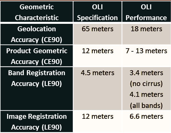
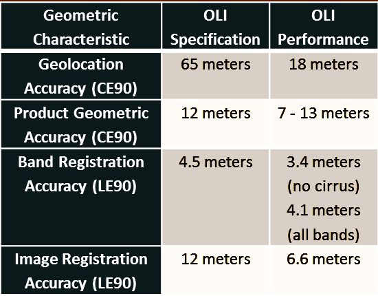
Geodetic accuracy refers to the absolute geolocation accuracy of OLI imagery and is measured using ground control points. The effects of terrain are compensated in the geodetic accuracy analysis so it reflects horizontal positional accuracy and is specified and measured in terms of 90% circular error (CE90). As noted in Table 1, the required accuracy is 65 meters (CE90) or better.

Geodetic accuracy statistics are collected when ground control points are correlated with OLI imagery as part of Level 1T product generation processing (using the GLS control) and also for the geometric calibration sites where higher accuracy DOQ and SPOT-derived control points are available. Every available control point of the selected type is correlated with a Level 1T OLI image generated using the spacecraft ephemeris (position and velocity) and attitude information provided in the Level 0 data stream. The control points that correlate successfully are analyzed to select a consistent set. The selected points are then used to compute ephemeris and attitude corrections. These corrections are applied to the geometric model and the final Level 1T product is then generated using the refined control-corrected model. As a byproduct of this procedure the computed correction values are stored in the IAS trending database for subsequent use in OLI-to-spacecraft alignment calibration. The control point statistics are also stored in the database to provide a record of the measured geolocation accuracy of the original OLI image. These statistics are analyzed to assess Landsat 8 geodetic accuracy.

The accuracy of the ground control used to evaluate the accuracy of the imagery is a concern if the control is less than an order of magnitude or so more accurate than the imagery. This is the case with the GLS control which is less than two-times more accurate (38 meter CE90) than the Landsat 8 geodetic accuracy specification (65 meter CE90). This problem is highlighted by comparing the geodetic accuracy results observed for the operational GLS control versus the calibration site control. It would be tempting to dismiss the GLS control for accuracy evaluation purposes on this basis, but it is important to recall that although the calibration site control provides better accuracy than the GLS control, it does not provide a global distribution of test sites. Relying solely on the calibration sites could mask the effects of systematic errors such as within-orbit thermally induced alignment variations. It is thus important to analyze both the highly accurate DOQ and the globally distributed GLS results.

Figure 8 shows the measured CE90 geodetic accuracy performance, summarized by calendar quarter, using three classes of ground control: (1) the GLS control used operationally to create Level 1T data products; (2) the DOQ/SPOT control used at calibration sites for geometric analyses; and (3) a subset of the GLS control referred to as anchor site control. The anchor sites are the Landsat Worldwide Reference System 2 (WRS-2) path/row locations that were controlled, with the assistance of the National Geospatial Intelligence Agency (NGA), during the global Landsat image triangulation that established the geometric framework for the GLS [8]. Since the NGA-provided control was not available everywhere around the world (e.g., not for many isolated islands), the GLS is not of uniform accuracy. Selecting sites that were used as the original GLS positional constraints ought to provide a globally distributed subset of sites that is more reliable than the overall GLS population.

Figure 8. OLI absolute geodetic/geolocation accuracy by calendar quarter. Anchor sites are the subset of Global Land Survey (GLS) scenes that contained control points provided by the National Geospatial Intelligence Agency (NGA).

Figure 8. OLI absolute geodetic/geolocation accuracy by calendar quarter. Anchor sites are the subset of Global Land Survey (GLS) scenes that contained control points provided by the National Geospatial Intelligence Agency (NGA).

As expected, the calibration site DOQ/SPOT-derived control reports much better accuracy than does the less accurate GLS control and the GLS anchor sites produce consistently better results than the remainder of the GLS control. Given the divergence in the results yielded by the different classes of ground control, establishing a single, defensible, estimate for Landsat 8 OLI geolocation accuracy requires separating the error components that are attributable to the OLI imagery from those that are due to the ground control itself. Consider the measured geolocation accuracy to be composed of four components:

$${\sigma }_{Net}^2={\sigma }_{CalBias}^2+{\sigma }_{DynCal}^2+{\sigma }_{Pointing}^2+{\sigma }_{GCP}^2$$

(4)

where:

(1)

${\sigma }_{CalBias}$ is static calibration error resulting from residual alignment calibration bias;

(2)

${\sigma }_{DynCal}$ is dynamic calibration error that varies with position due to within-orbit alignment changes;

(3)

${\sigma }_{Pointing}$ is random pointing error including spacecraft position and attitude knowledge, sensor internal line-of-sight stability, and alignment instability;

(4)

${\sigma }_{GCP}$ is ground control point error, including ~0.1 pixel GCP mensuration error.

If we can estimate the first three terms on the right hand side of Equation (4) we can produce an estimate of geolocation accuracy that is independent of the control point effects. We estimate the static calibration error by computing the mean geodetic offsets for all test scenes. This error component is treated as a constant offset. Dynamic calibration errors, in the form of within-orbit thermally induced alignment changes, are modeled as a linear trend in the mean offsets with position in orbit, using WRS row location as a proxy for orbit position. This error component can then be treated as a uniform error distribution varying between the maximum and minimum values it can attain across a given WRS row range.

Since the ground control point errors are fixed for a given site whereas the pointing errors should vary randomly for that site, we can estimate the random pointing error by analyzing the repeatability of the measured geodetic offsets at each WRS path/row. The standard deviations of the mean geodetic errors for all scenes over each path/row were computed for all scenes where there was more than one successful acquisition. The root-mean-squares of the site-specific standard deviations in each direction were taken to be estimates of the low frequency pointing error. Higher frequency within-scene pointing errors were estimated from the standard deviations of the scene-by-scene control point measurements at calibration sites. The low- and high-frequency estimates are root-sum-squared to yield a combined random pointing error estimate.

This error estimation approach was applied to both the GLS and calibration site/DOQ ground control point results collected during L1T processing, yielding the results shown in Table 3. In the GLS case, the residual calibration error terms (calibration bias and trend with WRS row) were estimated using only the anchor sites as there is some evidence of the presence of latitude-dependent systematic errors in the broader GLS. The pointing repeatability analysis included the entire GLS data set to obtain a larger sample. The implied GLS GCP error, however, applies only to the anchor sites.

The variance of a uniformly distributed random variable, X, that takes on values between min(X) and max(X) is [9]:

$${\sigma }^2={\left(\text{max}\left(X\right)-\text{min} (X)\right)}^2/12$$

(5)

Table 3. Landsat 8 global geolocation accuracy performance estimate. The final estimate is highlighted in bold in the table.

Source		GLS Scenes	DOQ Scenes	All Scenes
Static Calibration Error	Along-Track Mean (m)	2.9	0.2	2.9
	Across-Track Mean (m)	−2.0	−0.1	−2.0
Dynamic Calibration Trend	Along-Track Trend (m/row)	−0.076	−0.030	−0.076
	Across-Track Trend (m/row)	0.177	0.132	0.177
Calibration Trend Lever Arm	Row Range (rows)	94	57	124
Dynamic Calibration Error	Along-Track (m)	2.1	0.5	2.7
	Across-Track (m)	4.8	2.2	6.4
Random Pointing Error	Along-Track (m)	8.0	6.4	6.4
	Across-Track (m)	7.9	7.4	7.4
L8 Geolocation Error	CE90 (m)	19.0	15.1	18.1
Measured Geodetic Error	CE90 (m)	34.9	15.3	-
Implied GCP Error	CE90 (m)	29.2	2.3	-

Table 3. Landsat 8 global geolocation accuracy performance estimate. The final estimate is highlighted in bold in the table.

Source		GLS Scenes	DOQ Scenes	All Scenes
Static Calibration Error	Along-Track Mean (m)	2.9	0.2	2.9
	Across-Track Mean (m)	−2.0	−0.1	−2.0
Dynamic Calibration Trend	Along-Track Trend (m/row)	−0.076	−0.030	−0.076
	Across-Track Trend (m/row)	0.177	0.132	0.177
Calibration Trend Lever Arm	Row Range (rows)	94	57	124
Dynamic Calibration Error	Along-Track (m)	2.1	0.5	2.7
	Across-Track (m)	4.8	2.2	6.4
Random Pointing Error	Along-Track (m)	8.0	6.4	6.4
	Across-Track (m)	7.9	7.4	7.4
L8 Geolocation Error	CE90 (m)	19.0	15.1	18.1
Measured Geodetic Error	CE90 (m)	34.9	15.3	-
Implied GCP Error	CE90 (m)	29.2	2.3	-

Since the dynamic calibration term is being modeled as a linear trend with position in orbit, the range of values that it takes on is the trend, in terms of meters per WRS row, times the number of rows spanned by the data. The dynamic calibration contribution was thus computed as:

$${\sigma }_{DynCal}=\sqrt{{\left(trend\times row range\right)}^2/12}$$

(6)

The final Landsat 8 CE90 geolocation error was calculated from the individual components as follows:

$$Geolocation Error CE90=\sqrt{\begin{array}{c}{\sigma }_{CalBias AT}^2+{\sigma }_{CalBias XT}^2\\ +{\left(2.146\times \frac{\left({\sigma }_{DynCal AT}+{\sigma }_{DynCal XT}\right)}{2}\right)}^2\\ +{\left(2.146\times \frac{\left({\sigma }_{Pointing AT}+{\sigma }_{Pointing XT}\right)}{2}\right)}^2\end{array}}$$

(7)

The along- and across-track static calibration error terms are root-sum-squared along with the average of the along- and across-track terms for the dynamic calibration and pointing components, both of the latter being scaled by a factor of 2.146 to convert a root-mean-square value to 90% circular error. The implied control point error is computed as the root-sum-square difference between the measured CE90 geodetic error (shown in Table 3 and plotted in Figure 8) and the Landsat 8 geolocation error estimate. Note from Table 3 that the GLS and DOQ Landsat 8 geolocation accuracy estimates are reasonably close although the DOQ results exhibit smaller within-orbit effects due to their more restricted geographic distribution. Both analyses yielded reasonable values for the implied control point error based upon the expected accuracy of these control sources. The final estimate of global Landsat 8 geolocation error (the “All Scenes” column in Table 3) was calculated using the GLS estimates for static and dynamic calibration error (which require a global distribution of data to estimate accurately), the DOQ estimates for pointing error (which should be the same everywhere), and a WRS row range of 124, spanning a full daylight half-orbit. The result is an estimate of Landsat 8 geodetic accuracy of just over 18 meters (CE90), which is well below the 65 meter requirement. It is also better than the implied accuracy of the GLS control. This excellent geolocation accuracy leads to the somewhat unexpected conclusion that Level 1Gt products that do not use the GLS ground control will, in many cases, have better absolute accuracy, though poorer multi-temporal consistency, than L1T products.

3.2. Geometric Accuracy

The Landsat 8 geometric accuracy requirement refers to the accuracy of Level 1T products, after the application of ground control. This 12-meter CE90 requirement was intended to control the internal geometric accuracy of OLI images and was specified to be based upon GPS-quality ground control points and digital elevation data with accuracy commensurate with the Shuttle Radar Topography Mission (SRTM). From the previous section it should be apparent that ground control point accuracy will be a more important driver of operational Level 1T product accuracy than will Landsat 8 image geometry. 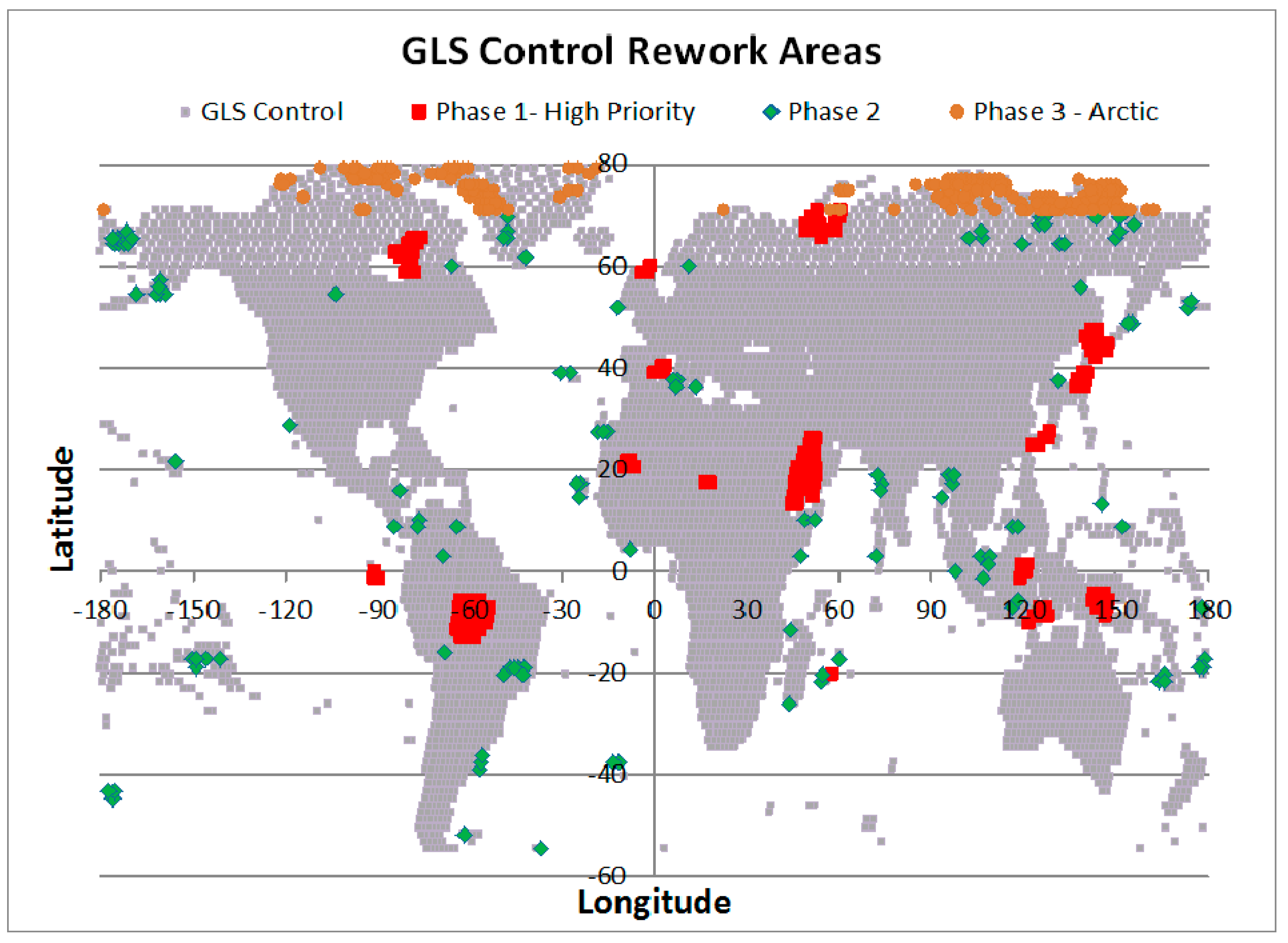This requirement has thus come to be considered in two contexts: (1) verification of the original 12-meter CE90 geometric accuracy requirement using calibration sites; and (2) characterization of Level 1T product accuracy relative to the GLS ground control framework, which is itself nominally accurate to 25 meters net root-mean-squared error (RMSE) or, equivalently, 38 meters CE90 [5]. It is worth noting that the excellent geolocation accuracy of Landsat 8 has made it possible to identify regions where the GLS control has substantially larger than expected errors. The worst of these are in the process of being improved, as is briefly described below.

At the time the GLS control point database was created, sites that contained a sufficiently large number of control points had a subset of the points identified as verification points. These verification points, which are not used in control point correction, are correlated with the final Level 1T product to measure its accuracy relative to the GLS geometric framework. These statistics are collected in the IAS trending database for every Level 1T product for which verification points are available.

Landsat 8 system internal geometric accuracy is evaluated at calibration sites using both high precision DOQ/SPOT-derived control and the GLS verification point results for those sites. Figure 9 shows a plot of the Level 1T geometric accuracy results by calendar quarter for four different combinations of control point source and scene type: (1) DOQ/SPOT control at calibration sites; (2) GLS verification points at calibration sites; (3) GLS verification points at anchor sites; and (4) the global set of GLS verification points. Table 4 shows the summary results for these four cases.

Table 4. Landsat 8 Level 1T product accuracy estimates.

Control Source	Scene Type	Number of Scenes	Level 1T Accuracy (CE90 Meters)
DOQ (post-fit residuals)	Calibration Site	352	6.7
GLS (verification points)	Calibration Site	640	7.8
GLS (verification points)	Anchor Site	6804	11.7
GLS (verification points)	All	78,962	12.6

Table 4. Landsat 8 Level 1T product accuracy estimates.

Control Source	Scene Type	Number of Scenes	Level 1T Accuracy (CE90 Meters)
DOQ (post-fit residuals)	Calibration Site	352	6.7
GLS (verification points)	Calibration Site	640	7.8
GLS (verification points)	Anchor Site	6804	11.7
GLS (verification points)	All	78,962	12.6

Figure 9. Level 1T product accuracy by calendar quarter. The accuracy estimates are highly sensitive to the quality of the ground control used to measure the accuracy.

Figure 9. Level 1T product accuracy by calendar quarter. The accuracy estimates are highly sensitive to the quality of the ground control used to measure the accuracy.

The calibration site results derived from high-quality control points span the first year of operations and are well below the requirement threshold of 12 meters. It should be noted that these scenes are screened for cloud cover prior to being processed whereas GLS results are generated for every scene that achieves an acceptable control point fit, regardless of cloud cover which could impact the ability to correlate verification points. The GLS results show both a seasonal variation in accuracy, believed to be due to increased cloud and snow interference in the northern hemisphere winter, and performance across the full global database that exceeds the 12-meter requirement. These results show that, as was the case with geolocation accuracy, the accuracy of the GLS control limits the accuracy of the final Landsat 8 Level 1T data products. This further justifies the ongoing effort to improve the quality of the GLS control.

3.3. Band Registration Accuracy

Band-to-band registration accuracy characterizes the alignment of the nine OLI spectral bands contained in each Level 1T product. Band-to-band registration performance is measured by cross-correlating all pair-wise subsets of the spectral bands using cloud-free acquisitions of characterization sites selected to minimize inter-band spectral differences. These are mostly desert sites with little vegetation and high altitude sites where the cirrus band is able to see ground features.

It was originally believed that the cirrus band signal from the Earth’s surface would be so attenuated by atmospheric water vapor absorption that it would never provide a usable image signal for band registration. The Landsat 8 IAS was thus equipped with processing software that performs the band registration assessment measurements using lunar scan data. Each lunar scan provides usable data for only a portion of one FPM. The lack of coverage for the full FPM field of view makes the lunar data less desirable for band alignment calibration purposes than Earth-view data. Band alignment in the lunar data can also be biased by residual scan rate errors, making it less reliable than Earth-view data for band registration characterization. When spectral simulations of the OLI cirrus band showed that usable Earth signals could be expected for high altitude sites under dry atmospheres, the OLI calibration plan was modified to use Earth-image band registration measurements for all spectral bands.

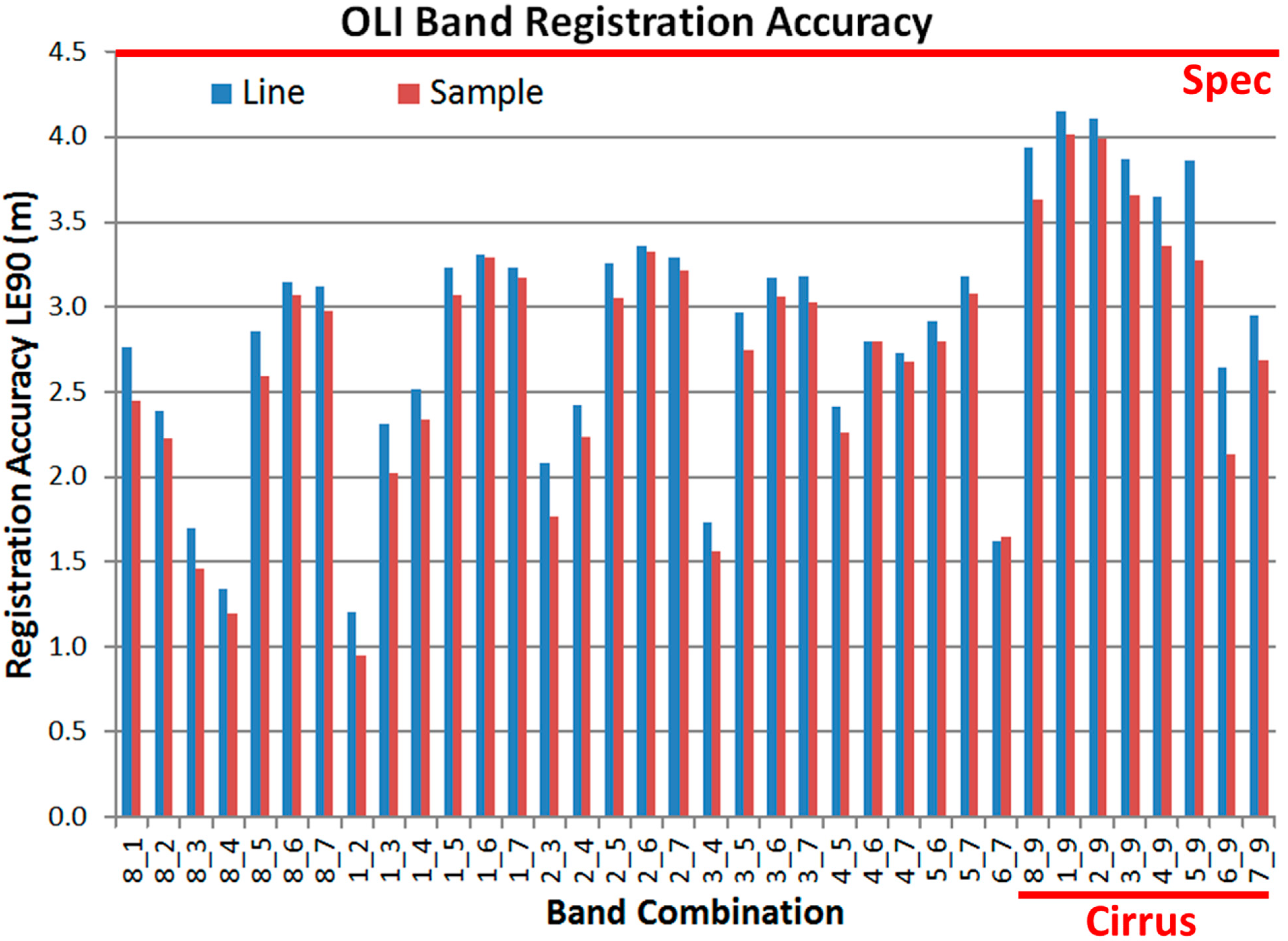
OLI band registration accuracy performance for Level 1T products is required to be better than 4.5 meters (LE90) in both the line and sample directions, for all spectral band-pairs. Figure 10 shows that the measured performance is below the requirement threshold for all band-pair combinations, and is well below the threshold for all band-pairs that do not include the cirrus band. Table 5 summarizes the OLI band registration accuracy results for all bands except the cirrus band and for the complete set of OLI bands, including the cirrus band. Note that although the number of scenes available for cirrus band characterization is limited, it is still larger than the number of lunar scans conducted during the same time period. Even in scenes that are usable for cirrus band characterization the signal levels are relatively low, so the registration uncertainty is greater for the cirrus band that it is for the other bands.

Figure 10. OLI band-to-band registration accuracy by band pair. Pairs including the cirrus band are grouped at the right end of the plot.

Figure 10. OLI band-to-band registration accuracy by band pair. Pairs including the cirrus band are grouped at the right end of the plot.

Table 5. OLI band registration accuracy, with and without the cirrus band. Both all-band average and worst case band-pair results are shown.

		Band RMS (LE90 Meters)		Worst Band Pair (LE90 Meters)
Band Set	Number of Scenes	Line	Sample	Line	Sample
Excluding Cirrus Band	482	2.7	2.6	3.4	3.3
All Bands	29	3.7	3.4	4.1	4.0

Table 5. OLI band registration accuracy, with and without the cirrus band. Both all-band average and worst case band-pair results are shown.

		Band RMS (LE90 Meters)		Worst Band Pair (LE90 Meters)
Band Set	Number of Scenes	Line	Sample	Line	Sample
Excluding Cirrus Band	482	2.7	2.6	3.4	3.3
All Bands	29	3.7	3.4	4.1	4.0

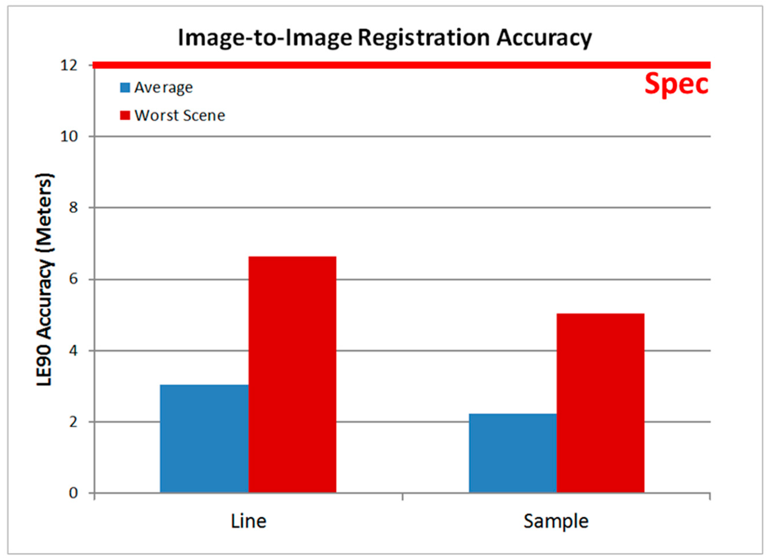
3.4. Image Registration Accuracy

In addition to characterizing the geometric accuracy of Level 1T products as described above, the internal geometric accuracy of OLI images is evaluated by measuring the alignment of Level 1T products acquired over the same site over time. Image-to-image registration accuracy, which is specified to be 12 meters (LE90) or better in the line and sample directions, is characterized by correlating pairs of Level 1T products over the same WRS path/row. The earliest-acquired cloud-free image of a given test site is chosen as a reference image that is compared to subsequent acquisitions. The resulting registration accuracy assessment is less sensitive to the quality of the ground control and verification points since it is a direct comparison of two OLI images, albeit images that have both been corrected using the GLS ground control. This characterization uses cloud-free images over a set of test sites selected to provide a good north-south geographic distribution in order to look for performance differences associated with position in orbit.

Figure 11 shows a graphical depiction of the measured image registration accuracy results from 128 scenes acquired over 10 test sites. Note that even the worst-case scene measured as of March 2014 was well within the required accuracy.

Figure 11. OLI image-to-image registration accuracy; blue bars—average over all test scenes; red bars—worst-case test scene.

Figure 11. OLI image-to-image registration accuracy; blue bars—average over all test scenes; red bars—worst-case test scene.

Table 6 shows the accuracy values corresponding to the plot. It should be noted that these results, derived from 15-meter ground sample distance panchromatic band data, are approaching the accuracy limitations (0.1 to 0.2 pixel) of the image correlation tools used to measure the image-to-image displacements.

Table 6. OLI multi-temporal image-to-image registration accuracy results.

All Scene RMS (LE90 Meters)		Worst Scene (LE90 Meters)		Specification (LE90 Meters)
Line	Sample	Line	Sample	Line	Sample
3.052	2.250	6.623	5.051	12	12

Table 6. OLI multi-temporal image-to-image registration accuracy results.

All Scene RMS (LE90 Meters)		Worst Scene (LE90 Meters)		Specification (LE90 Meters)
Line	Sample	Line	Sample	Line	Sample
3.052	2.250	6.623	5.051	12	12

4. Discussion and Ongoing Work

The Landsat 8 OLI geometric calibration program—spanning the pre-launch, commissioning, and operational phases of the mission and described in Section 2—was designed to provide knowledge of the key sensor and spacecraft geometric parameters required by the OLI geometric model. This knowledge, coupled with the inherent stability of the OLI instrument, has resulted in Landsat 8 data product geometric performance, documented in Section 3, which meets or exceeds all of the original requirements. The software tools used to perform the on-orbit calibration and characterization operations are implemented in the IAS—a core component of the Landsat 8 ground system—and are thus available for ongoing performance monitoring and calibration refinement. The IAS also provides a development environment for advanced algorithms and new or improved geometric processing and analysis techniques. An example of how the IAS capabilities are being leveraged to improve the accuracy of the Landsat ground control point library is briefly described below.

Following the successful on-orbit geometric calibration campaign during the commissioning period, all aspects of Landsat 8 OLI geometric performance continue to be significantly better than requirements. Table 7 shows a summary of the measured Landsat 8 performance compared to the original requirements. The corresponding performance levels for Landsat 7 were tabulated previously in Table 1. The operational on-orbit characterization and calibration capabilities of the Landsat 8 IAS ensure that geometric performance is continually monitored and that accuracy is maintained. This on-orbit calibration and characterization activity will continue for the life of the mission. Since the end of the commissioning period, only two small adjustments to the OLI-to-spacecraft alignment, noted in Table 2, have been required to maintain the current level of performance. No changes to the calibration of the OLI’s internal geometry have been necessary.

Table 7. Landsat 8 OLI geometric performance summary.

Characteristic	OLI Specification	OLI Performance	Notes
Absolute Geodetic Accuracy (CE90)	65 meters	18 meters	See Table 3.
Geometric (Level 1T Product) Accuracy (CE90)	12 meters	7 to 13 meters	Depends on ground control quality. See Table 4.
Band Registration Accuracy (LE90)	4.5 meters	3.4 meters (no cirrus) 4.1 meters (all bands)	Worst direction, worst band-pair. See Table 5.
Image Registration Accuracy (LE90)	12 meters	6.6 meters	Worst direction, worst scene. See Table 6.

Table 7. Landsat 8 OLI geometric performance summary.

Characteristic	OLI Specification	OLI Performance	Notes
Absolute Geodetic Accuracy (CE90)	65 meters	18 meters	See Table 3.
Geometric (Level 1T Product) Accuracy (CE90)	12 meters	7 to 13 meters	Depends on ground control quality. See Table 4.
Band Registration Accuracy (LE90)	4.5 meters	3.4 meters (no cirrus) 4.1 meters (all bands)	Worst direction, worst band-pair. See Table 5.
Image Registration Accuracy (LE90)	12 meters	6.6 meters	Worst direction, worst scene. See Table 6.

One fact noted in Table 7 that became apparent during the course of OLI geometric performance characterization is that Level 1T product accuracy is currently limited by the quality of the GLS ground control point network. The 18-meter CE90 Landsat 8 absolute geolocation accuracy is better than the 25-meter radial RMSE specification (38 meters CE90) of the GLS and thus of the control derived from the GLS. The Landsat 8 product generation philosophy of basing all products on the GLS control framework was chosen intentionally to favor consistency across the Landsat archive over absolute accuracy. That being said, actual system performance was not expected to be as good as it is, and the excellent Landsat 8 geolocation accuracy is now being leveraged to improve the accuracy of the GLS control in the most problematic areas in order to improve the quality of the entire Landsat archive.

Figure 12 shows a global plot of the areas scheduled for control improvement. Note that many of these areas are islands or high latitude areas where NGA-provided control was not available to support GLS construction. The first phase of the control point improvement activity is focused on 15 areas identified as high priority due to the presence of large (at least one scene over 75 meters) temporally consistent offsets between Landsat 8 and the GLS control. Satellite block triangulation techniques are being used to update the GLS control in these areas using multiple OLI acquisitions. The triangulation solution is weighted to ensure that the problematic areas are adjusted to improve their accuracy while remaining consistent with the surrounding unadjusted areas. At least one scene in each rework area is checked against high resolution commercial satellite image data. This control improvement activity is expected to continue through 2014 as the remaining phase 2 and phase 3 areas are worked. Once all of the control point position updates are completed, the control point library will be refreshed by extracting new OLI image chips to supplement the existing Landsat 7 GLS-derived data.

Figure 12. Landsat 8 ground control improvement sites. The 15 highest priority areas are shown in red, second priority areas are shown in green, and high latitude areas are shown in tan.

Figure 12. Landsat 8 ground control improvement sites. The 15 highest priority areas are shown in red, second priority areas are shown in green, and high latitude areas are shown in tan.

5. Conclusions

The success of the Operational Land Imager (OLI) geometric calibration program is demonstrated by the geometric accuracy performance of the Landsat 8 data products. The measured worst-case band registration accuracy of 4.1 meters LE90 (versus a requirement of 4.5 meters LE90) across all band pairs, which had been considered one of the more challenging requirements, is especially gratifying since the OLI sensor architecture makes this aspect of performance particularly reliant on accurate calibration and careful geometric modeling and data correction processing. The geolocation accuracy achieved (18 meters CE90 versus a 65 meter requirement) has motivated work on new techniques that seek to use Landsat 8 data to improve the accuracy of the entire Landsat archive. Implementing the on-orbit geometric calibration and characterization capabilities in a core component of the Landsat 8 ground system, facilitates on-going performance monitoring and will ensure that future changes in performance are detected and, if appropriate, compensated by calibration updates.

References

1. Irons, J.; Dwyer, J.; Barsi, J. The next Landsat satellite: The Landsat data continuity mission. Remote Sens. Environ. 2012, 122, 11–21. [Google Scholar] [CrossRef]
2. Knight, E.J.; Kvaran, G. Landsat-8 operational land imager design, characterization and performance. Remote Sens. 2014, 6, 10286–10305. [Google Scholar] [CrossRef]
3. NASA. Landsat Data Continuity Mission Operational Land Imager Requirements Document—Revision E; NASA Goddard Space Flight Center: Greenbelt, MD, USA, 2009.
4. Storey, J.; Choate, M.; Lee, K. Geometric performance comparison between the OLI and the ETM+. In Proceedings of 2008 Pecora 17—The Future of Land Imaging Going Operational, Denver, CO, USA, 18–20 November 2008; pp. 18–20.
5. Gutman, G.; Huang, C.; Chander, G. Assessment of the NASA-USGS Global Land Survey (GLS) datasets. Remote Sens. Environ. 2013, 134, 249–265. [Google Scholar] [CrossRef]
6. Micijevic, E.; Morfitt, R.; Choate, M. Landsat 8 on-orbit characterization and calibration system. Proc. SPIE 2011. [Google Scholar] [CrossRef]
7. USGS. LDCM Cal/Val Algorithm Description Document—Version 3.0; U.S. Geological Survey: Sioux Falls, SD, USA, 2013.
8. Dykstra, J.D.; Storey, J.C. Landsat-7 definitive ephemeris-an independent verification of GeoCover-Ortho 1990 positional accuracy. In Proceedings of 2004 the ASPRS Annual Conference, Denver, CO, USA, 23–28 May 2004. (CD_ROM).
9. Fisher, L. Probability and statistics. In Handbook of Applied Mathematics, 2nd ed.; Van Nostrand Reinhold Company: New York, NY, USA, 1983; pp. 1217–1273. [Google Scholar]