Assessing Band Sensitivity to Atmospheric Radiation Transfer for Space-Based Retrieval of Solar-Induced Chlorophyll Fluorescence

Abstract

In contrast to ground-based solar-induced chlorophyll fluorescence (Fs) detection, the influence of atmospheric radiation transfer is the major difficulty in Fs retrieval from space. In this study, we first simulated top-of-atmosphere (TOA) radiance using FluorMODgui3.1 and MODTRAN5 code. Based on the simulated dataset, we analyzed the sensitivities of five potential Fs retrieval bands (Hα, K I, Fe, O₂-A, and O₂-B) to different atmospheric transfer parameters, including atmosphere profile, aerosol optical depth (AOD₅₅₀), vertical water vapor column (H₂O), vertical ozone column (O₃), solar zenith angle (SZA), view zenith angle (VZA), relative azimuth angle (RAA) and elevation. The results demonstrate that the Hα, O₂-A and O₂-B bands are the most sensitive to these atmospheric parameters. However, only the O₂-A and O₂-B bands were found to be sensitive to the imaging geometric parameters. When the spectral resolution was sufficient, the K I and Fe bands proved to have the best potential for space-based Fs retrieval given the current available accuracies of atmospheric products, while the O₂-A band was shown to perform better at lower spectral resolutions. The band sensitivity analysis presented here will be useful for band selection and atmospheric correction for space-based Fs retrieval.

1. Introduction

Solar-induced chlorophyll fluorescence (Fs) refers to the emission of radiation by chlorophyll molecules. It is strongly related to the status of the photosynthetic process [1,2]. Numerous experiments have demonstrated that, as an indicator of photosynthesis, Fs can be used to obtain physiological information about plants in a non-invasive, fast, and sensitive manner [3,4,5,6].

To extract Fs from measured at-sensor radiance signals, it is necessary to decouple the reflected solar flux and emitted Fs. A comprehensive overview of current methods of estimating Fs was provided by Meroni et al. [7]. Most of the commonly used methods are based on the Fraunhofer Line Depth principle (FLD) [8], which compares the downward solar irradiance and the upward canopy radiance at bands inside and outside the solar Fraunhofer lines or atmospheric absorption bands. The standard FLD method relies on the assumption that the reflectance and Fs are constants (wavelength independent) within the employed spectral window [8]; however, in reality, this assumption is not strictly true. To overcome this weakness of the standard FLD method, other more accurate methods such as 3FLD [9] and improved FLD (iFLD) [10] have been proposed. These methods have been widely used in Fs detection at the canopy level [11,12,13].

In order to detect Fs at the regional or global scale, methods based on satellite remote sensing are indispensable. The FLuorescence EXplorer (FLEX) mission has been selected as a candidate for ESA’s Earth Explorer 8 mission. If finally selected, the FLuORescence Imaging Spectrometer (FLORIS) will fly in formation with Sentinel-3 in a sun-synchronous orbit at a height of approximately 815 km [14]. The proposal of the FLEX mission will aim to highlight research on space-based Fs retrieval. However, the algorithms designed for use at ground level cannot be applied directly to space-based Fs retrieval because the upward radiance observed by the satellite remote sensor is strongly influenced by absorption and scattering in the atmosphere. Assessment of the band sensitivity to atmospheric influence for Fs detection is, therefore, required. The Fs spectral range covers the region approximately from 650 to 800 nm with two peaks at approximately 685 nm and 740 nm [1]. This spectral window includes several solar Fraunhofer lines, together with the O₂-A and O₂-B absorption bands [15]. Space-based Fs retrieval was first carried out by Guanter et al. in a small region in Spain using MERIS data from the O₂-A absorption band [16]. Guanter et al. simulated a data set from a FLEX-like measurement to test and develop algorithms (including FLD and SFM) for Fs retrieval in the O₂-A and O₂-B bands, and also analyzed the sensitivity of the top-of-atmosphere (TOA) radiance to different atmospheric parameters in the two bands [17]. Compared with the O₂ absorption bands, the solar Fraunhofer lines are much less influenced by atmospheric absorption. The hyperspectral data from TANSO-FTS onboard GOSAT has a high spectral resolution of approximately 0.02 nm in the range of 755–775 nm and hence several solar Fraunhofer lines near the Fs peak at 740 nm can be detected. The K I line centered at 770.1 nm has also been employed to retrieve Fs at global or regional scales [18,19]. Frankenberg et al. employed two spectral windows, centered at 755 nm and 770 nm, which covered several Fe lines (the deepest one centered at 758.8 nm) and the K I line, to reduce the algorithm’s sensitivity to instrument noise [20]. In addition to the bands mentioned above, the Hα line centered at 656.5 nm has also been employed for Fs detection but only at ground level [21,22]. This line is much broader than the K I or Fe lines but suffers from several H₂O absorption features.

As mentioned above, several solar Fraunhofer lines and atmospheric absorption bands have the potential to be used for space-based Fs retrieval but the influence of atmospheric radiation transfer on them varies according to the band. Guanter et al. provided an evaluation of atmospheric effects on Fs retrieval uncertainties for the O₂-A and O₂-B bands, but an analysis for solar Fraunhofer lines was not included [17]. Frankenberg et al. and Guanter et al. claimed that the solar Fraunhofer lines were less affected by the disturbance due to the atmosphere [20,23]. Damm et al. analyzed Fs retrieval biases related to observational and atmospheric parameters for the O₂-A band for the case of a diurnal experiment [24]. In practice, the accuracy of the atmospheric parameters used depends on the configuration (e.g., signal-to-noise ratio and spectral resolution) of atmospheric observation instruments and retrieval algorithms. Therefore, it is of vital importance to assess the potential of different bands for space-based Fs retrieval given the accuracy of currently available atmosphere products (e.g., the MODIS atmosphere products).

The purpose of this study is to quantify the sensitivity of space-based Fs retrieval in different bands and to assess the potential of these bands given the accuracy of available remotely sensed atmospheric products. According to earlier studies that were reviewed by Meroni et al. (2009) [7], the Hα line, the Fe line centered at 758.8 nm, the K I line, the O₂-A band and the O₂-B band located at 650–775 nm have the potential for Fs retrieval, so these bands and lines were selected for this study. Four atmospheric parameters (atmospheric profile, aerosol optical depth, vertical water vapor column, and vertical ozone column) and four imaging geometric parameters (solar zenith angle, view zenith angle, relative azimuth angle and the elevation) were investigated in this study. The results can serve as a reference for band selection for space-based Fs retrieval.

2. Materials and Methods

2.1. Experiments of Simulation

In order to analyze the band sensitivity to atmospheric radiation transfer for space-based Fs retrieval, the true values of Fs and the atmospheric parameters (under different atmospheric conditions) are needed. To meet this requirement, we used simulated TOA radiance spectra based on FluorMODgui v3.1 [25,26] and MODTRAN5 [27] in this study.

Assuming that both Fs and the surface reflectance follow Lambert’s cosine law, the TOA radiance can be expressed as [17],

$$L_{TOA}=L_0+\frac{[(E_{dir}{\mu }_s+E_{dif}){\rho }_s/\pi +Fs]T_{\uparrow }}{1-S{\rho }_s}$$

(1)

where L₀ is the atmospheric path radiance, E_dir and E_dif are the direct and diffuse fluxes of solar irradiance arriving at the surface, μ_s is the cosine of the solar zenith angle, ρ_s is the surface reflectance, S is the atmospheric spherical albedo and T_↑ is the total transmittance of the atmosphere.

The top-of-canopy (TOC) Fs and reflectance were simulated using FluorMODgui v3.1 with a spectral resolution (SR) of 1 nm. FluorMOD is a physical model that provides reliable simulations of the reflected radiance and also the fluorescence emitted by the canopy. This model has been widely used in the assessment of Fs retrieval methods [28,29,30]. By analyzing the 120 samples in the LOPEX’93 dataset [31], we found that the leaf chlorophyll content was always in the range of 20 μg/cm² to 80 μg/cm². The values of leaf chlorophyll were, therefore, set as 20, 40, 60 and 80. Following the work of Damm et al. [29], the values of LAI were set as 1, 2, 4, and 6, and the values of fluorescence quantum efficiency were set as 0.02 and 0.04. As a result, there were 32 different datasets, including TOC Fs and reflectance spectra, obtained by using different combinations of values of the three parameters. All other parameters required by FluorMODgui were set to their default values. Details of the parameters used are listed in Table 1.

Table 1. Input leaf and canopy parameters used in the FluorMODgui canopy fluorescence model [26].

Parameter	Value	Units	Description
LAI	1, 2, 4, 6	-	Leaf area index
N	1.5	-	Leaf internal structure parameter
Cab	20, 40, 60, 80	μg/cm2	Leaf chlorophyll a + b content
Cw	0.025	cm	Leaf water content
Cm	0.01	mg/cm2	Leaf dry matter content
Fi	0.02, 0.04	-	Fluorescence quantum efficiency
T	20	°C	Temperature
Sto	2	-	Stoichiometry of PS II to PS I
PAR b	0.0035	-	Electron transport resistance
PAR re	0.005	-	Heat dissipation constant
h	0.1	-	Hot-spot size parameter
LIDF a, LIDF b	−0.5, 0.5	-	Leaf inclination distribution function, abs(LIDFa) + abs(LIDFb) < 1, spherical (a = −0.35, b = −0.15), planophile (a = 1, b = 0) erectophile (a = −1, b = 0), plagiophile (a = 0, b = −1) extremophile (a = 0, b = 1), uniform (a = 0, b = 0)

Table 1. Input leaf and canopy parameters used in the FluorMODgui canopy fluorescence model [26].

Parameter	Value	Units	Description
LAI	1, 2, 4, 6	-	Leaf area index
N	1.5	-	Leaf internal structure parameter
Cab	20, 40, 60, 80	μg/cm2	Leaf chlorophyll a + b content
Cw	0.025	cm	Leaf water content
Cm	0.01	mg/cm2	Leaf dry matter content
Fi	0.02, 0.04	-	Fluorescence quantum efficiency
T	20	°C	Temperature
Sto	2	-	Stoichiometry of PS II to PS I
PAR b	0.0035	-	Electron transport resistance
PAR re	0.005	-	Heat dissipation constant
h	0.1	-	Hot-spot size parameter
LIDF a, LIDF b	−0.5, 0.5	-	Leaf inclination distribution function, abs(LIDFa) + abs(LIDFb) < 1, spherical (a = −0.35, b = −0.15), planophile (a = 1, b = 0) erectophile (a = −1, b = 0), plagiophile (a = 0, b = −1) extremophile (a = 0, b = 1), uniform (a = 0, b = 0)

The atmospheric parameters that appear in Equation (1) were calculated using the MODTRAN5 code for the 650–775nm spectral window. The spectral resolution of the MODTRAN5 simulations was set as 0.02 nm, which is similar to the spectral resolution of TANSO-FTS onboard GOSAT. MODTRAN5 code can calculate the TOA radiance and atmospheric transmittance when provided with the necessary atmospheric parameters, imaging geometric parameters and surface reflectance. The atmospheric radiation transfer parameters in Equation (1) can then be derived with algebra [32]. In this study, we investigated four kinds of atmospheric parameters including the atmospheric profile (AP), aerosol optical depth at 550 nm (AOD₅₅₀), vertical water vapor column (H₂O), and vertical ozone column (O₃); and four imaging geometric parameters, including the solar zenith angle (SZA), view zenith angle (VZA), relative azimuth angle (RAA) and elevation. The expected values and ranges of the atmospheric parameters were determined according to their global variations [33,34] and the MODIS global aerosol product, MOD04_L2 [35]. The expected values and ranges of the imaging geometric parameters were set according to the common imaging conditions of currently operational sensors (Table 2). We did not take the aerosol model used or the type of cloud into account because space-based Fs detection is generally performed for rural regions and under clear weather conditions.

Table 2. The expected values and ranges of parameters used for atmospheric radiation transfer modeling by MODTRAN5 under different conditions.

Parameters	Unit	Expected Value	Range
AP	-	MLS	TA, MLS, MLW, SAS, SAW, USS *
AOD550	-	0.3	0.1–1.0
O3	DU	300	200–450
H2O	g∙cm−2	3	0.1–6
SZA	deg	30	25–35
VZA	deg	15	10–20
RAA	deg	90	70–110
Elevation	m	50	0–100

* Abbreviations for atmospheric profiles used in the table: “TA” is the tropical atmosphere, “MLS” is Mid-latitude summer, “MLW” is Mid-latitude winter, “SAS” is Sub-arctic summer, “SAW” is Sub-arctic winter, and “USS” is the 1976 US standard atmosphere.

Table 2. The expected values and ranges of parameters used for atmospheric radiation transfer modeling by MODTRAN5 under different conditions.

Parameters	Unit	Expected Value	Range
AP	-	MLS	TA, MLS, MLW, SAS, SAW, USS *
AOD550	-	0.3	0.1–1.0
O3	DU	300	200–450
H2O	g∙cm−2	3	0.1–6
SZA	deg	30	25–35
VZA	deg	15	10–20
RAA	deg	90	70–110
Elevation	m	50	0–100

* Abbreviations for atmospheric profiles used in the table: “TA” is the tropical atmosphere, “MLS” is Mid-latitude summer, “MLW” is Mid-latitude winter, “SAS” is Sub-arctic summer, “SAW” is Sub-arctic winter, and “USS” is the 1976 US standard atmosphere.

According to data measured by subnanometer resolution spectroradiometer [36], the reflectance spectra were continuous and smooth in the visible and near-infrared band. According to the simulated data of FluorMOD [26] and SCOPE [37], the Fs spectra were also continuous and smooth. We, therefore, resampled the simulated reflectance and Fs spectra by spline to match the SR of the MODTRAN5 outputs. We then derived the simulated TOA radiance using a spectral resolution similar to that of spectra observed by GOSAT for different leaf/canopy and atmospheric conditions, and we also obtained the true values of Fs.

2.2. Selection of Potential Bands

Near the Fs spectral peaks at 685 nm and 740 nm, there are several solar Fraunhofer absorption lines and telluric atmospheric absorption bands that have the potential for space-based Fs retrieval; however, the solar Fraunhofer lines and the telluric atmospheric absorption bands have different characteristics. Solar Fraunhofer lines are usually very narrow and hence these lines can be detected only using data with sufficiently high SR. However, for isolated solar Fraunhofer lines, the influence of the atmospheric radiation transfer is relatively weak. This is a distinct advantage in space-based Fs retrieval. In comparison, the O₂-A and O₂-B absorption bands are much broader, which means that the two bands can be much more easily detected and will have lower sensitivity to the signal-to-noise ratio (SNR). Obviously, however, the influence of atmospheric radiation transfer must be treated carefully when these bands are employed for Fs retrieval using remotely sensed data.

According to the spectral resolution of current space-based spectrometers (such as band 1 of GOSAT-FTS, which covers 755–775 nm with a spectral resolution of approximately 0.02 nm [38], and channel 4 of GOME-2, which covers 590–790 nm with a spectral resolution of approximately 0.5 nm [39]) and Modtran5, we selected five commonly used bands: Hα, Fe, K I, O₂-A, and O₂-B. The detailed characteristics of the five bands are listed in Table 3. Note that, for simplicity, in this paper, the name “Fe” is used only to refer to the specific Fe line centered at 758.8 nm.

Table 3. List of characteristics for the five selected bands.

Band Name	Absorption Depth	Wavelength (nm)
		Left Shoulder	Center	Right Shoulder
Hα	81%	654.36	656.46	657.90
K I	42%	770.02	770.12	770.20
Fe	33%	758.76	758.82	758.90
O2-A	92%	758.00	761.00	767.70
O2-B	59%	686.60	687.10	690.50

Table 3. List of characteristics for the five selected bands.

Band Name	Absorption Depth	Wavelength (nm)
		Left Shoulder	Center	Right Shoulder
Hα	81%	654.36	656.46	657.90
K I	42%	770.02	770.12	770.20
Fe	33%	758.76	758.82	758.90
O2-A	92%	758.00	761.00	767.70
O2-B	59%	686.60	687.10	690.50

2.3. Fs Retrieval Methods

2.3.1. Space-Based Fs Retrieval Algorithm

In this study, three commonly used Fs retrieval algorithms (FLD, 3FLD, and iFLD) were tested. For satellite remotely sensed data, they needed to be modified a little to deal with the atmospheric radiation transfer parameters.

First, the TOA radiance was transferred to the TOC radiance:

$$\begin{array}{l}L=\frac{L_{TOA}-L_0}{T_{\uparrow }}\\ I=\frac{1}{\pi }(E_{dir}{\mu }_s+E_{dif})+L·S\end{array}\}$$

(2)

where L is the upward radiance at the TOC and I is the downward radiance that reaches the TOC. By substituting Equation (2) in Equation (1), Equation (1) was transferred to:

$$L=I{\rho }_s+Fs$$

(3)

All variables in Equation (2) can be calculated using the MODTRAN5 code as explained in Section 2.1. The problem of space-based Fs retrieval, therefore, turned out to be same as ground-level retrieval of Fs.

Using the standard FLD method [8] and assumption that the values of both Fs and the reflectance are constant over the narrow spectral range considered, Fs can be calculated using two bands (one at the center of the absorption line and one outside the line for reference) as:

$$Fs=\frac{I_{out}{L}_{in}-I_{in}{L}_{out}}{I_{out}-I_{in}}$$

(4)

where the subscripts “in” and “out” refers to the bands inside and outside the absorption line, respectively.

To overcome the weak assumptions of the standard FLD method, Maier et al. proposed the 3FLD method [9]. In the 3FLD method, it is assumed that the variation of Fs and the reflectance over the spectral range is linear. The weighted average of two bands to the left and right of the absorption line is then used as the reference rather than a single band that lies outside the line, as in the FLD method. The weights of the two bands are defined as:

$$w_{left}=\frac{{\lambda }_{right}-{\lambda }_{in}}{{\lambda }_{right}-{\lambda }_{left}},\text{ and }{w}_{right}=\frac{{\lambda }_{in}-{\lambda }_{left}}{{\lambda }_{right}-{\lambda }_{left}}$$

(5)

where w_left and w_right are the weights of the bands on the left and right shoulder of the absorption band. Then Equation (4) can be expressed as:

$$Fs=\frac{(I_{left}{w}_{left}+I_{right}{w}_{right})L_{in}-I_{in}(L_{left}{w}_{left}+L_{right}{w}_{right})}{[(I_{left}{w}_{left}+L_{right}{w}_{right})-I_{in}]}$$

(6)

Alonso et al. proposed the improved FLD (iFLD) method, which made use of hyperspectral data to account for a nonlinear variation in both Fs and the reflectance within the spectral window [10]. In the iFLD method, Fs is expressed as:

$$Fs=\frac{{\alpha }_R{I}_{out}{L}_{in}-I_{in}{L}_{out}}{{\alpha }_R{I}_{out}-{\alpha }_F{I}_{in}}$$

(7)

where α_R and α_F are the ratios of the reflectance to Fs outside and inside the absorption line, respectively. Their values can be estimated as:

$${\alpha }_R\approx \frac{{\tilde{R}}_{out}}{{\tilde{R}}_{in}},\text{ and }{\alpha }_F\approx \frac{I_{out}}{{\tilde{I}}_{in}}{\alpha }_R$$

(8)

where R̃_in and R̃_out are the apparent reflectance inside and outside the absorption line and Ĩ_in is obtained by interpolating the value of I in order to remove the absorption feature (refer to [10] for details).

2.3.2. Comparison of Fs Retrieval Methods

The performance of the three commonly used Fs retrieval methods varies, especially under different SNR conditions for the five employed bands. For the purpose of this study, we needed to select an optimum Fs retrieval method to investigate the sensitivity of different bands to atmospheric effects. We therefore compared the Relative Root Mean Square Error (RRMSE) of the three methods for five bands under different SNR conditions using TOC radiance.

In order to simulate radiance with different SNRs, we added random Gaussian-distributed noise with a mean value of zero to the simulated radiance (repeated 100 times for each spectrum). The SNR is defined as the ratio of the signal intensity to the standard deviation of the random Gaussian-distributed noise, and the SNR values of 50, 100, 200, 300, 400 and 500 were used.

As Figure 1 shows, the standard FLD method produced relatively high values of the RRMSE and standard deviation for Fs retrieval for all five bands under noise-free conditions, whereas the 3FLD and iFLD methods apparently increased the accuracy of the Fs retrieval. The RRMSEs of Fs retrieved using the two methods are all less than 20%.

Figure 2 shows the RRMSE for the three Fs retrieval methods for five bands under different SNR conditions. For all methods and all bands, the RRMSE clearly increases as the SNR decreases, especially when the SNR is less than 200. For all five bands, the iFLD method has the highest sensitivity to the SNR. Overall, the most similar results for the five different bands were obtained using the 3FLD method and this method also has a low sensitivity to the SNR. We, therefore, selected the 3FLD method to investigate the sensitivity of the different bands to atmospheric effects.

Figure 1. Values of the Relative Root Mean Square Error (RRMSE) and standard deviation of the retrieved solar-induced chlorophyll fluorescence (Fs) obtained using three methods for five bands under noise-free conditions. The values of the RRMSE and standard deviation were calculated using 32 different simulated “true” value of Fs.

Figure 1. Values of the Relative Root Mean Square Error (RRMSE) and standard deviation of the retrieved solar-induced chlorophyll fluorescence (Fs) obtained using three methods for five bands under noise-free conditions. The values of the RRMSE and standard deviation were calculated using 32 different simulated “true” value of Fs.

Figure 2. The RRMSE for Fs retrieval using Fraunhofer Line Depth principle (FLD) (a), 3FLD (b) and improved FLD (iFLD) (c) for different bands with SNRs of 50, 100, 200, 300, 400 and 500, and also for the noise-free case. The RRMSE values were calculated using 32 different simulated “true” values of Fs for each SNR condition. Note that the ranges of the RRMSE in the three parts of the figure are not the same.

Figure 2. The RRMSE for Fs retrieval using Fraunhofer Line Depth principle (FLD) (a), 3FLD (b) and improved FLD (iFLD) (c) for different bands with SNRs of 50, 100, 200, 300, 400 and 500, and also for the noise-free case. The RRMSE values were calculated using 32 different simulated “true” values of Fs for each SNR condition. Note that the ranges of the RRMSE in the three parts of the figure are not the same.

2.4. Analysis of the Sensitivity of Fs Retrieval to Atmospheric Radiative Transfer

To retrieve Fs accurately from space, the first and most important step is to obtain accurate values of the atmospheric radiation transfer parameters that appear in Equation (2). The values of these parameters depend on the inputs to the atmospheric radiation transfer codes, such as MODTRAN5. These inputs include atmospheric parameters and imaging geometric parameters, including those listed in Table 2.

Because of the limited accuracy of current atmospheric products produced by space-based instruments (e.g., the bias of MODIS atmospheric products is about 5%–15% [35,40,41]), it is usually impossible to get absolutely accurate values of the required atmospheric parameters (including the atmospheric profile, aerosol optical depth, vertical water vapor column, and vertical ozone column). This means that estimated values from different data sources have to be used. The values of the imaging geometric parameters such as the solar zenith angle, view zenith angle, relative azimuth angle and the elevation can be measured with sufficient accuracy. However, a pixel-by-pixel atmospheric correction based on these parameters would be a very time-consuming task that may be not feasible in practice. Look-up tables of the atmospheric radiation transfer parameters are commonly used to overcome this problem. It is, therefore, important to quantify the sensitivity to the atmosphere of the bands that are commonly used in space-based Fs retrieval.

Following the work of Damm et al. [24], we assessed the sensitivity of Fs retrieval to atmospheric radiative transfer for different bands using the Local Sensitivity Analysis (LSA) method. In this method, a Jacobian matrix J was calculated as:

$$J={\left[j_k\right]}_{1\le k\le m},with{j}_k=\frac{\delta F{s}_{rel}}{\delta pa{r}_{norm,k}}$$

(9)

where J is the matrix of the partial derivatives of the retrieved relative Fs (Fs_rel) with respect to the normalized atmospheric or imaging geometric parameters (par_norm), and m is the number of the parameters analyzed. δFs_rel was calculated as:

$$\delta F{s}_{rel}=\frac{\left|F{s}_{pert}-F{s}_{exp}\right|}{F{s}_{exp}}$$

(10)

where Fs_exp is the Fs retrieved from TOA spectra simulated using the expected values of parameters (mean output of 32 simulations), and Fs_pert is the Fs retrieved from TOA spectra simulated using the perturbed parameters. As the parameters have different units, they were normalized according to:

$$pa{r}_{norm}=\frac{par}{pa{r}_{\max }-pa{r}_{\min }}$$

(11)

We calculated the Jacobian matrix numerically for AOD₅₅₀, H₂O, O₃, SZA, VZA, RAA and the elevation by perturbing each input parameter in the TOA spectra simulation by 10% of its usual range (see Table 2). Therefore, the sensitivity of the retrieved Fs to parameter par_k can be described by the value of element j_k of the Jacobian matrix.

In contrast, the sensitivity to the atmospheric profile cannot be calculated numerically. However, we found that only the mid-latitude winter (MLW) and sub-arctic winter (SAW) profiles led to different results from the other atmosphere profiles for the five bands studied. So the relative difference between Fs retrieved from TOA spectra simulated with the mid-latitude Summer (MLS) and MLW profiles was used to describe the band sensitivity to the atmosphere profile according to:

$$Sen{s}_{atm}=\frac{\left|F{s}_{MLS}-F{s}_{MLW}\right|}{F{s}_{MLS}}$$

(12)

where Fs_MLS is the Fs retrieved from TOA spectra simulated using the mid-latitude summer atmosphere profile, and Fs_MLW is the Fs retrieved from TOA spectra simulated using the mid-latitude winter profile.

3. Results

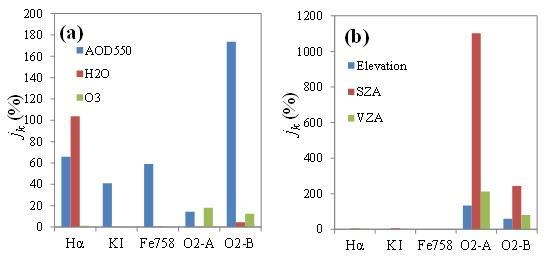
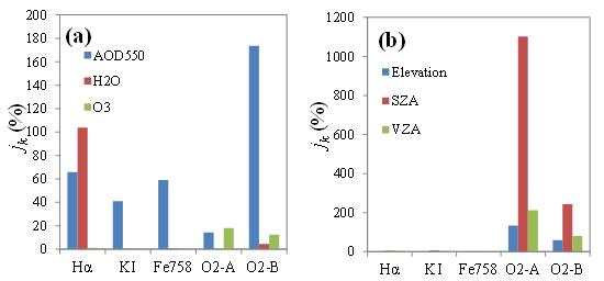
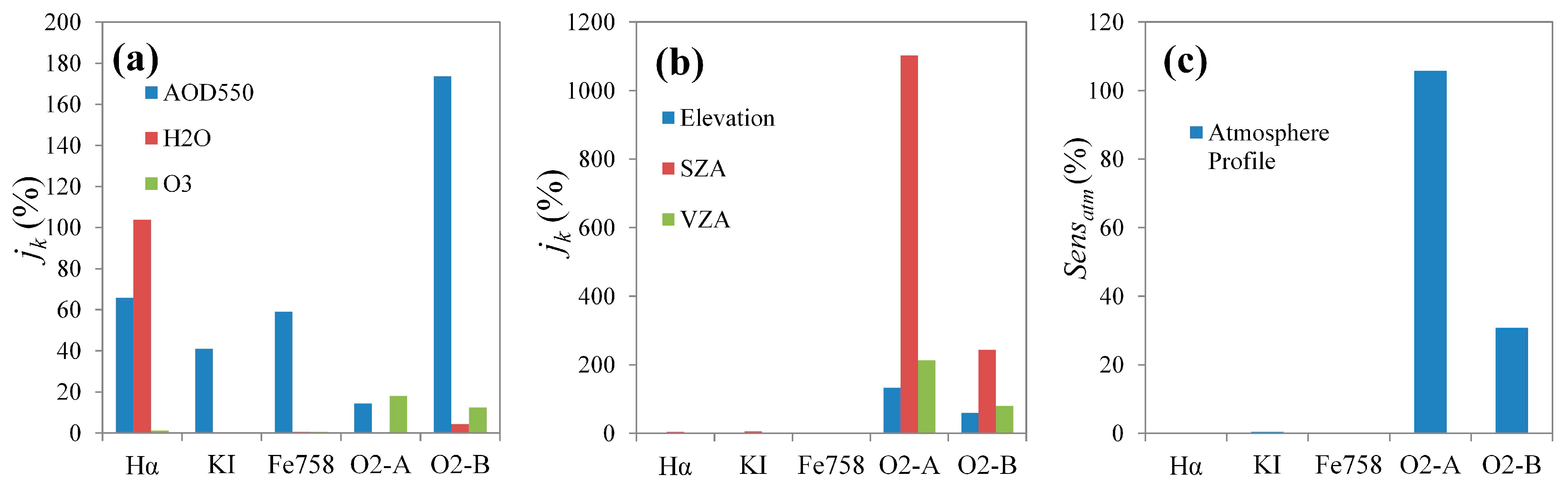
3.1. Sensitivity of Different Bands to Atmospheric Parameters and Imaging Geometric Parameters

Using Equation (9), we quantified the sensitivity of the five different bands to the three atmospheric parameters and four imaging geometric parameters listed in Table 2. As explained in Section 2.3.2, the 3FLD method was selected to investigate the sensitivity, and all tests were run under noise-free conditions.

As Figure 3a shows, the value of AOD₅₅₀ has an obvious influence on all five bands. The O₂-B band is most greatly influenced by the value of AOD₅₅₀ (with sensitivities (j_k) of 173.63%). The value of AOD₅₅₀ influences the atmospheric transmittance, path radiance, and spherical albedo for the whole spectral region and causes the simulated upward and downward radiance at TOC (L and I) to change. Even though the AOD₅₅₀ has little influence on the relative depth of the solar Fraunhofer lines, it does have an influence on the retrieved value of Fs. The amount of H₂O has an obvious influence only on the Hα and O₂-B bands because there are several H₂O absorption lines in the spectral windows of these two bands. The value of O₃ has an obvious influence on the O₂-A and O₂-B bands only, with sensitivities of 18.06% and 12.46%. This means that the Hα, O₂-A and O₂-B bands are more sensitive to the values of the atmospheric parameters. For the other two bands, the aerosol optical depth is the main factor that needs to be considered in space-based Fs retrieval.

Figure 3. Sensitivity of different bands to atmospheric parameters (a); imaging geometric parameters (b); and atmosphere profiles (c). The sensitivities to the relative azimuth angle are not shown as they were always equal to zero within the ranges tested. Note that the definition of sensitivity to the atmosphere profile is different from that for the other parameters.

Figure 3. Sensitivity of different bands to atmospheric parameters (a); imaging geometric parameters (b); and atmosphere profiles (c). The sensitivities to the relative azimuth angle are not shown as they were always equal to zero within the ranges tested. Note that the definition of sensitivity to the atmosphere profile is different from that for the other parameters.

As Figure 3b shows, all the imaging geometric parameters except the RAA have a large influence on the O₂-A and O₂-B bands but have little influence on the solar Fraunhofer absorption bands (the sensitivities are less than 6%).

As Figure 3c shows, the choice of atmosphere profile has obvious influence only on the O₂-A and O₂-B bands.

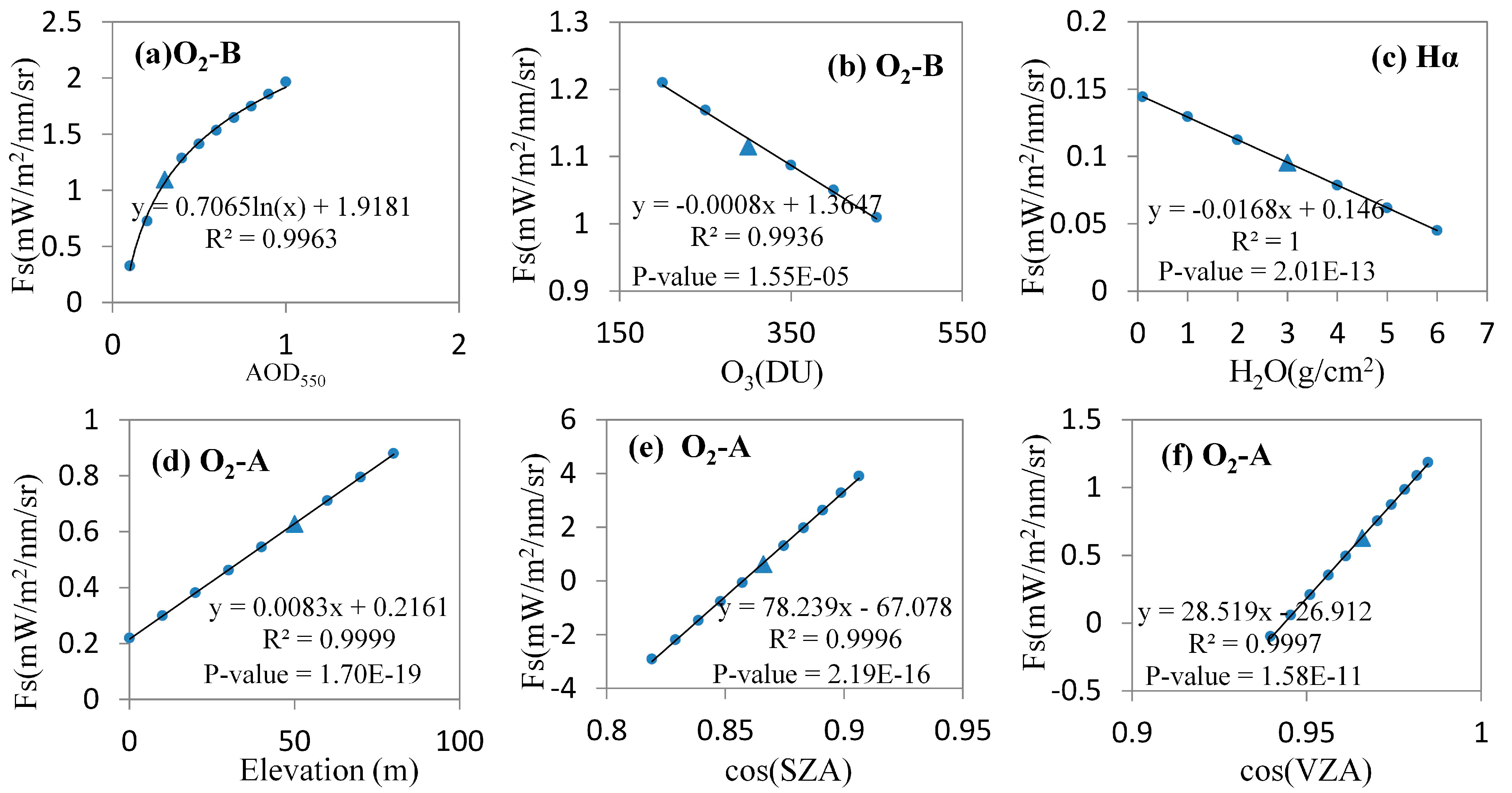
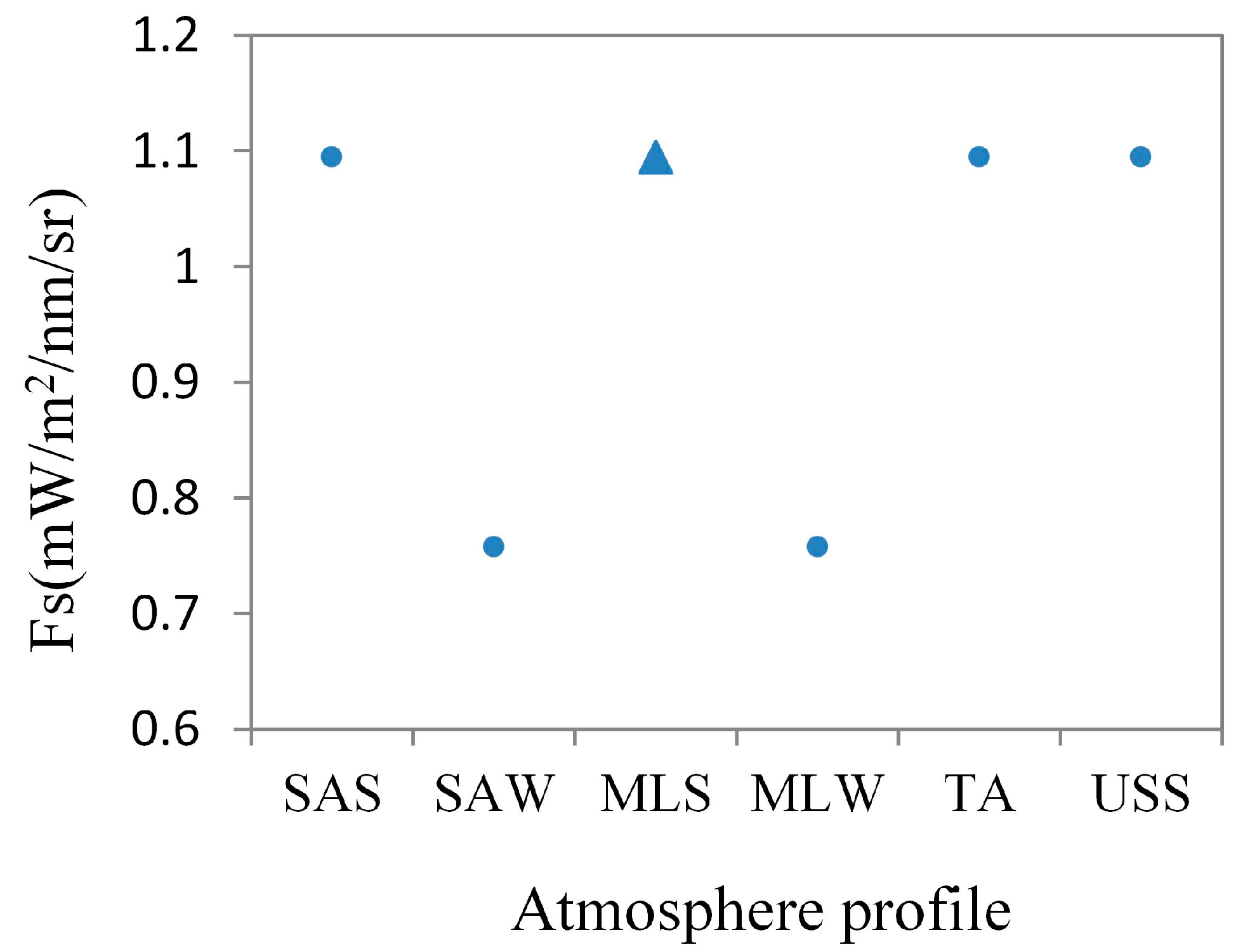
3.2. Relationship between Retrieved Fs and Parameters Used in TOA Radiance Simulation

We have demonstrated that the Hα, O₂-A and O₂-B bands are more sensitive to atmospheric and imaging geometric parameters, while the K I and Fe bands are apparently influenced by the aerosol optical depth only. In practice, it is hard to get accurate values of the necessary parameters at each sample point. We therefore investigated the relationship between the retrieved Fs values and the “real” values of parameters used in the simulation of TOA radiance to assess the feasibility of relatively accurate Fs retrieval based on interpolated atmospheric radiation transfer parameters.

The strong correlations (coefficient of determination higher than 0.99 and p-value lower than 10⁻⁴) between the retrieved Fs values and the values of parameters used in the simulation of TOA radiance are illustrated in Figure 4 for the most sensitive band for each of six parameters (AOD₅₅₀, H₂O, O₃, Elevation, SZA, and VZA), for the ranges that we tested. Note that the analysis for each parameter was carried out within the ranges listed in Table 2, and all other parameters were set to the expected values. The analysis was performed only for bands with sensitivities higher than 5%.

Figure 4. Relationship between retrieved Fs values and the values of parameters used in the simulation of top-of-atmosphere (TOA) radiance. We selected the most sensitive band for each parameter to show the results: O₂-B band for AOD₅₅₀ (a) and O₃ (b); Hα band for H₂O (c); and O₂-A band for elevation (d), solar zenith angle (SZA) (e) and view zenith angle (VZA) (f). The triangles represent the Fs values retrieved with TOA radiance simulated using the “expected” parameter values.

Figure 4. Relationship between retrieved Fs values and the values of parameters used in the simulation of top-of-atmosphere (TOA) radiance. We selected the most sensitive band for each parameter to show the results: O₂-B band for AOD₅₅₀ (a) and O₃ (b); Hα band for H₂O (c); and O₂-A band for elevation (d), solar zenith angle (SZA) (e) and view zenith angle (VZA) (f). The triangles represent the Fs values retrieved with TOA radiance simulated using the “expected” parameter values.

The situation regarding the choice of atmosphere profiles is somewhat different. For the six atmosphere profiles examined in this study, only the MLW and SAW profiles led to a different result from the other atmosphere profiles for the five bands studied (as shown in Figure 5). Therefore, it was only necessary to consider two atmospheric profiles for mid-latitude and sub-arctic regions (i.e., summer or winter) and only one profile for tropical regions when the other parameters were fixed.

Figure 5. Retrieved Fs values from TOA radiance simulated using different atmospheric profiles in the O₂-B band.

Figure 5. Retrieved Fs values from TOA radiance simulated using different atmospheric profiles in the O₂-B band.

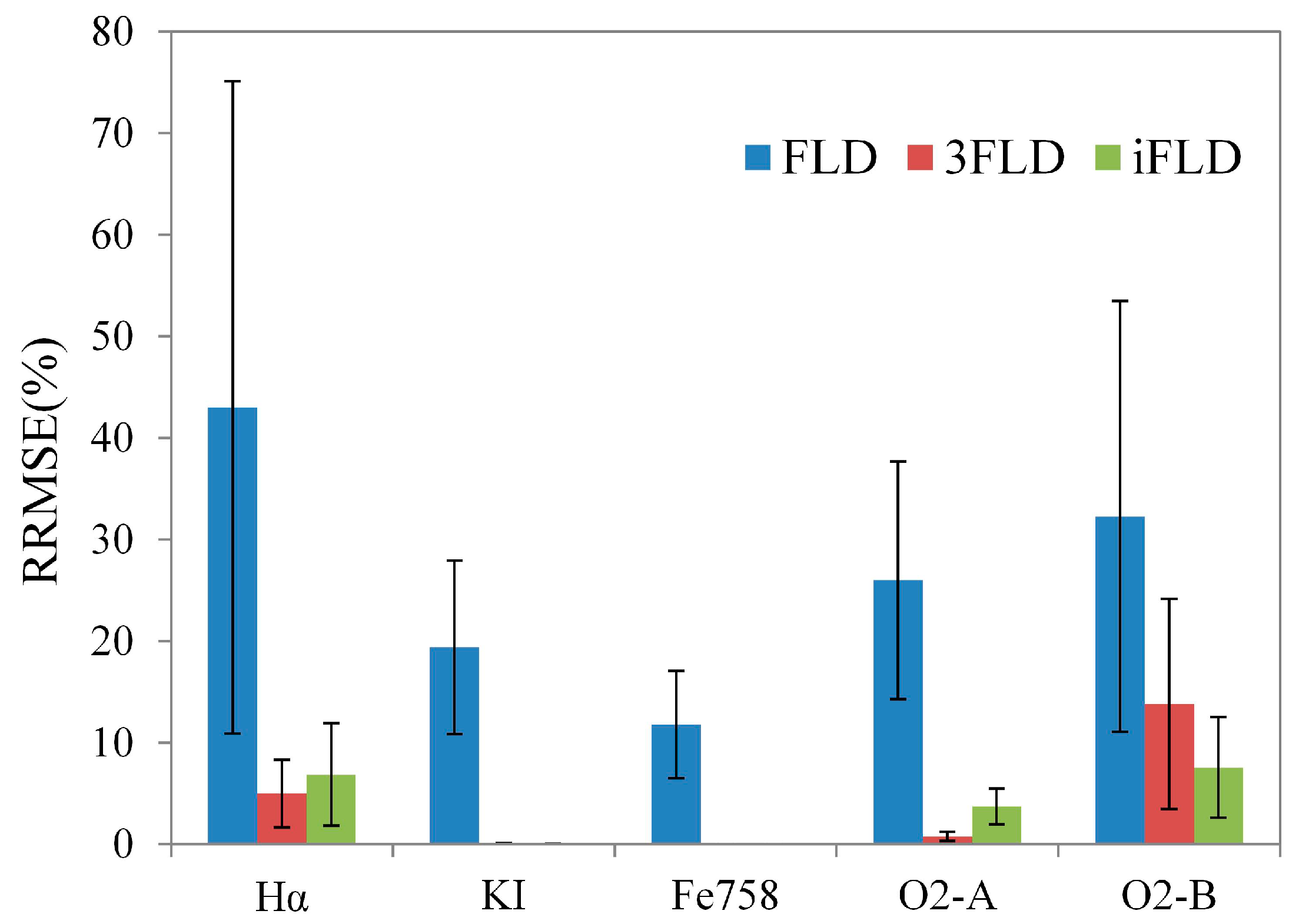
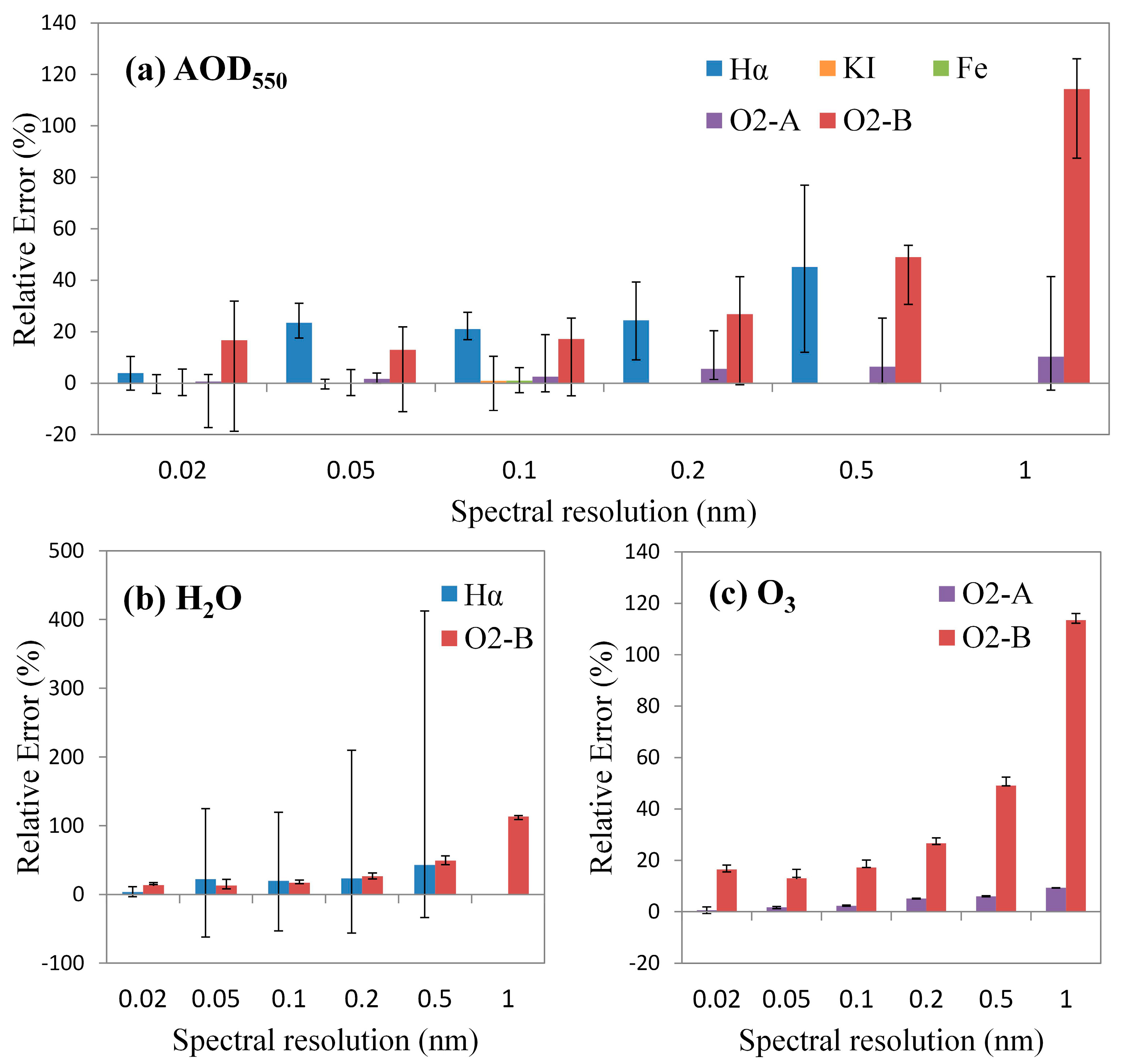
3.3. Errors in Fs Retrieval Based on Atmospheric Parameters with Currently Available Accuracy

The errors in retrieved Fs values are composed of systematic errors due to the algorithm used and errors due to inaccurate atmospheric correction. The accuracy of atmospheric parameters depends on the configuration of atmosphere observation instruments and the retrieval algorithm. We have demonstrated that the main atmospheric parameters that had an influence on the space-based Fs retrieval were AOD₅₅₀, H₂O and O₃. At the global scale, AOD₅₅₀ can be obtained from the MODIS aerosol product (MOD04_L2) [35]. The uncertainty in AOD₅₅₀ (Δτ) over land in MOD04_L2 is ± 0.05 ± 0.15τ [40]. H₂O can be retrieved from the MODIS precipitable water product (MOD05_L2) [42]. The uncertainty in the MOD05_L2 product is 5%–10% according to the work of Gao et al. [41]. O₃ can be retrieved from data from the Ozone Monitoring Instrument (OMI) onboard the Aura satellite [43,44]. Balis et al. validated the OMI total ozone column product and found that the bias was less than 5% [45]. Imaging geometric parameters can be measured quite accurately, so a consideration of these is not included in this section.

According to the current accuracy of the commonly used sources of the atmospheric parameters listed above, we set the bias in AOD₅₅₀, H₂O, and O₃ to ± 0.095, ± 0.3 g∙cm⁻², and ± 15 DU, respectively, relative to their expected values, and investigated the errors in the retrieved values of Fs due to the bias in the atmospheric parameters in the sensitive bands for different spectral resolutions. Figure 6 shows the relative errors of retrieved Fs with accurate atmospheric correction and the variation in the errors due to the bias in the atmospheric parameters. The results show that, with the currently available accuracy of the atmospheric parameters and the spectral resolution of GOSAT (0.02 nm), the relative errors in the values of Fs retrieved from the K I and Fe lines are below 5%; the relative error in Fs retrieved from the Hα line is below 12%; for Fs retrieved from the O₂-A band it is below 20%; and from the O₂-B band below 32%. The values of Fs retrieved from Hα, O₂-A and O₂-B bands are very sensitive to the spectral resolution. The O₂ absorption bands consist of many narrow absorption lines (width < 0.1 nm) and the Hα line is perturbed by some moisture absorption lines close to it. Therefore, the shapes of the absorption bands of the two O₂ bands and Hα line vary significantly at different spectral resolution (compared to their full width at half maximum (FWHM)). However, the shapes of the K I and Fe lines are not so sensitive to spectral resolution (also compared to their FWHM) for Fs retrieval if the absorption line is still observable (SR < 0.1 nm). Furthermore, it is quite challenging to accurately estimate the reflectance ratio and fluorescence ratio of the two bands inside and outside the absorption lines. The uncertainties in the estimates of the reflectance ratio and fluorescence ratio are much larger for the three “wide” (~1 nm) bands (O₂-B, O₂-A and Hα) than for the two “narrow” (<0.1 nm) lines (K I and Fe). Therefore, compared to the three “wide” bands, for Fs retrieval, the K I and Fe lines are not so sensitive to the spectral resolution (based on their FWHM) if the absorption feature is still observable. This indicates that, given a high enough spectral resolution, the K I and Fe lines would have more potential for space-based Fs retrieval using atmospheric products than can be achieved currently. For lower spectral resolutions, the O₂-A band has more potential than the O₂-B band.

Figure 6. Relative errors in retrieved Fs values for bands sensitive to AOD₅₅₀ (a); H₂O (b) and O₃ (c) under different spectral resolution. The error bars in the histograms represents the variation in the retrieval errors due to the bias in the atmospheric parameters. The K I and Fe lines could not be detected when the spectral resolution was lower than 0.1 nm and the Hα line could not be detected when the spectral resolution was lower than 0.5 nm.

Figure 6. Relative errors in retrieved Fs values for bands sensitive to AOD₅₅₀ (a); H₂O (b) and O₃ (c) under different spectral resolution. The error bars in the histograms represents the variation in the retrieval errors due to the bias in the atmospheric parameters. The K I and Fe lines could not be detected when the spectral resolution was lower than 0.1 nm and the Hα line could not be detected when the spectral resolution was lower than 0.5 nm.

4. Discussion

4.1. Assessment of Bands for Fs Retrieval

Most research on Fs retrieval at ground level has employed the O₂-A and O₂-B bands because these bands are relatively broad. The spectral resolution requirement is then low. However, the oxygen absorption features of the Earth’s atmosphere are greatly influenced by atmospheric radiation transfer and hence for space-based Fs retrieval the situation is much more complicated. To overcome the influence of the atmosphere, Frankenberg et al., for example, employed the isolated solar Fraunhofer lines to retrieve Fs values from space using GOSAT and OCO-2 data [20]. However, the solar Fraunhofer lines are much narrower than the O₂-A or O₂-B band, which means that a higher spectral resolution is needed, and, as a result, the sensitivity requirements for the sensors are higher.

Although it is clear that the solar Fraunhofer lines are less influenced by atmospheric radiation transfer, in terms of research into space-based Fs retrieval, quantitative assessment of band sensitivity based on the current accuracy of atmosphere products is useful, especially for band selection. In this paper, we assessed the sensitivities of five commonly used bands to nine atmospheric and imaging geometric parameters for space-based Fs retrieval. The K I and Fe solar Fraunhofer lines were found to be sensitive to aerosol optical depth only, while the Hα line was found, in addition, to be very sensitive to the vertical water vapor column because there are several water absorption lines surrounding it. The imaging geometric parameters (SZA, VZA, and elevation) had little influence on any of the solar Fraunhofer lines. The results also showed that the O₂-A and O₂-B bands are greatly influenced by the aerosol optical depth and imaging geometric parameters, while the O₂-B band is also sensitive to vertical water vapor and the ozone column. Among the eight tested parameters, the relative azimuth angle was found to have absolutely no influence on any of the bands within the ranges that were set. Given the current accuracy of commonly used atmospheric parameters and the spectral resolution of GOSAT, the uncertainty in Fs retrieval using the Hα, O₂-A, and O₂-B bands is much greater than the uncertainty that results from using the K I and Fe lines. These results are a consequence of the O₂-A and O₂-B bands being telluric atmosphere absorption bands, which are strongly influenced by atmospheric radiation transfer, especially the absorption of oxygen. Although the Hα line is a solar Fraunhofer line, it is perturbed by the moisture absorption lines around it. In contrast, as isolated solar Fraunhofer lines, the K I and Fe lines are little influenced by atmospheric radiation transfer. In addition, the spectral windows for Fs retrieval using the K I and Fe lines are much narrower, which leads to there being a smaller difference between the reflectance (or Fs) inside and outside of the absorption bands. This makes the basic assumption of 3FLD method (that the variation of Fs and the reflectance over the spectral window is linear) much stronger. In conclusion, if the spectral resolution is high enough, the K I and Fe solar Fraunhofer lines perform better in space-based Fs retrieval; if the spectral resolution is not sufficient to detect the K I or Fe lines, the O₂-A band will perform better.

However, it also needs to be noted that the band selection for Fs retrieval is also affected by the wavelength-dependent intensity of Fs. The O₂-B band is located at the Fs peak near 688 nm, while the Fe line, O₂-A band, and K I line are located near the 740 nm Fs peak. In contrast, the Hα line is located relatively far from Fs peaks and hence the intensity of Fs at the Hα line is quite weak, which may lead to relatively high errors in retrieved Fs values. As the results show, it is of vital importance to carry out accurate atmospheric correction in the course of research into, or applications of, space-based Fs retrieval using atmospherically sensitive bands. However, in this study we also found perfect correlations between the retrieved Fs values and the values of parameters used in the TOA radiance simulation. The reason behind this phenomenon is that the retrieved Fs value is related to the atmospheric radiation transfer parameters such as the atmospheric transmittance, spherical albedo and path radiance (see Equations (2) and (4)). The atmospheric radiation transfer procedure is also influenced by the atmospheric and imaging geometric parameters that we studied. Although it is difficult to give a detailed explanation for the correlations in this paper, this interesting phenomenon indicates the potential for carrying out atmospheric correction based on “sparser” look-up tables. However, this is only a theoretical study, and the situation is likely to be much more complex in practice.

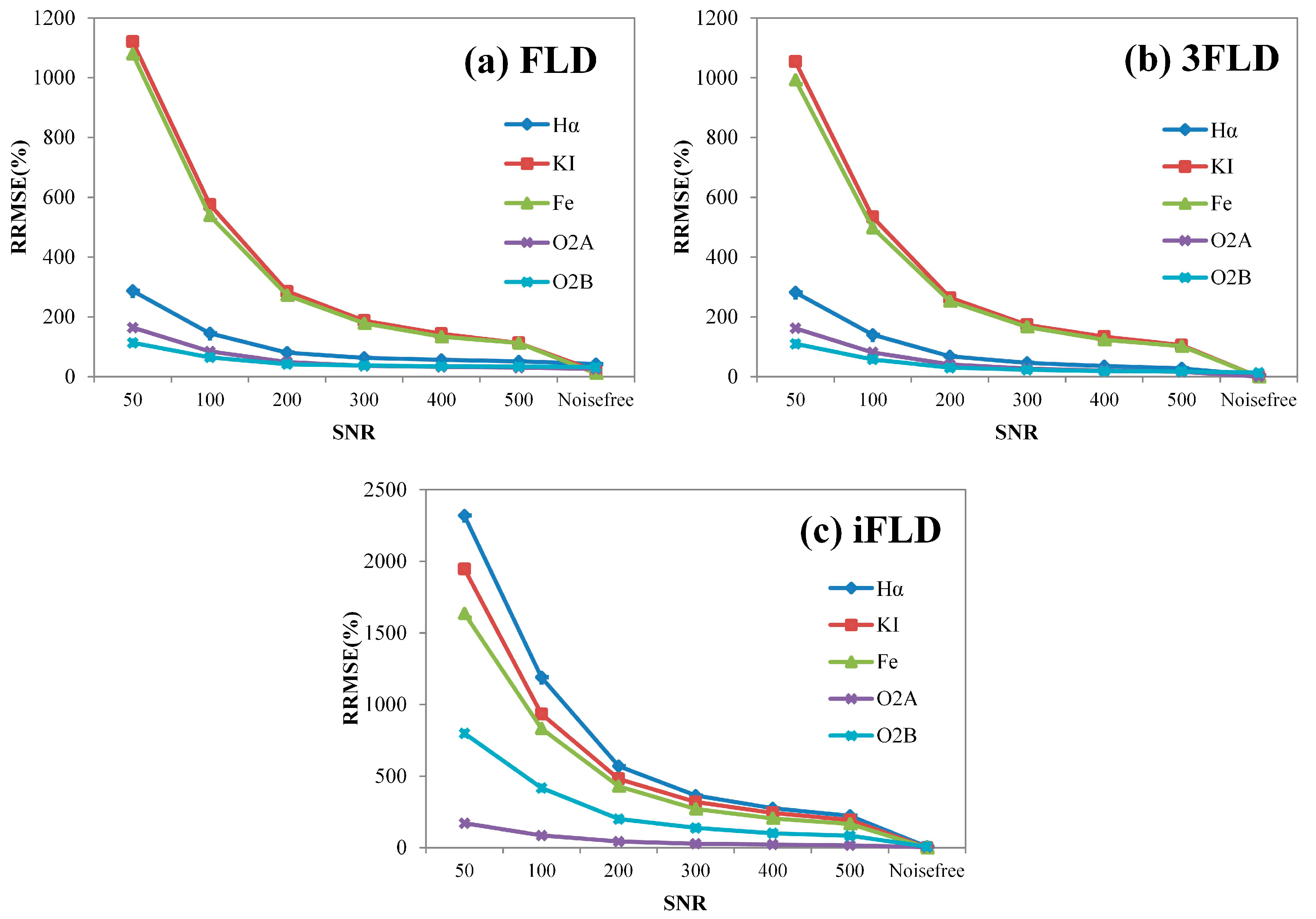
4.2. Uncertainty Analysis for Fs Retrieval

This study is dedicated to the analysis of band sensitivity to atmospheric radiation transfer, so other factors which will lead to Fs retrieval errors were not taken into account.

As Damm et al. showed, sensor configurations (such as SNR, spectral resolution, and spectral shift) are important parameters influencing the accuracy of Fs retrieval [29]. In this study, all data was simulated, and both the TOA simulation and the calculation of atmospheric radiation transfer parameters were carried out using the MODTRAN5 code. There was, therefore, no bias caused by mismatching of the spectral resolution between the TOA radiance and solar irradiance used for reference or any bias caused by a spectral shift. For the analysis of the sensitivity to atmospheric radiation transfer, we used noise-free data.

In order to quantify the band sensitivity to each parameter that was related to the atmospheric radiation transfer, in each test, we changed the value of one parameter only, keeping the values of the other parameters equal to their expected values. In practice, the situation is more complicated. Further investigations into the interactions between different parameters are still required.

The Ring effect caused by inelastic scattering such as Rotational Raman Scattering (RRS) can fill in the Fraunhofer lines in a similar way to the Fs [46]. The Ring effect is related to the imaging geometry and spectral resolution [47,48,49]. As Vasilkov et al. showed, for the condition SZA = 45° and VZA = 0°, the in-filling by Fs was larger than that due to RRS by a factor of about two at the center of the O₂-A band at high spectral resolution (FWHM = 0.03 nm), while at FWHM = 1.0 nm the factor was 6.4 [50]. Therefore, the uncertainty in retrieved Fs values due to RRS is larger for higher spectral resolutions. However, we did not take the influence of RRS into account in this study.

5. Conclusions

In this paper, we quantified the sensitivity of different bands to atmospheric radiation transfer for space-based Fs retrieval using data simulated by MODTRAN5 and FluorMODgui3.1. TOA radiance was simulated using different combinations of canopy, atmospheric and imaging geometric parameters to represent commonly encountered real-world conditions. The analysis of the sensitivity was carried out for three commonly used solar Fraunhofer absorption lines (Hα, K I, and Fe) and two Earth atmospheric absorption bands (O₂-A and O₂-B). Four atmospheric parameters (AP, AOD₅₅₀, O₃, and H₂O) and four imaging geometric parameters (SZA, VZA, RAA, and elevation) were selected for testing. We examined the accuracy of the FLD, 3FLD and iFLD methods for space-based Fs retrieval under different SNR conditions, and selected the 3FLD method to investigate the sensitivity of the bands.

On one hand, this study provided a quantitative assessment of band sensitivity to atmospheric radiation transfer for space-based retrieval of Fs. Although it is common knowledge that atmospheric absorption bands are much more strongly influenced by atmospheric perturbations than solar Fraunhofer lines, the results of this study can help to determine the required accuracy of the input parameters for space-based Fs retrieval using different bands. On the other hand, we investigated the uncertainty in the retrieved Fs values for different spectral resolutions for different bands, based on the accuracy of the available atmospheric products provided by MODIS and OMI. The results will be useful for band selection based on the known accuracy of available atmospheric parameters. Additionally, we also found that there were strong correlations between the retrieved Fs values and the parameters used in TOA radiance simulation, which indicates that there is potential for atmospheric correction based on “sparser” look-up tables.

However, this was still a theoretical examination based on simulated data. We avoided the errors caused by noise, spectral shift and the mismatching of spectral resolution between the TOA radiance and the solar irradiance used for reference. The parameters were analyzed separately and the interaction among them was not taken into account. The influence of the Ring effect was also neglected. It is important to carry out further investigations into these sources of uncertainty, and to find out precise physical explanations for the relationships founded in this paper. Additionally, it must be noted that, in practice, the selection of bands is related not only to the accuracy of the Fs retrieval but also to the intended application. When designing a spectrometer for Fs detection, the application potential of different bands must be considered carefully.

References

1. Baker, N.R. Chlorophyll fluorescence: A probe of photosynthesis in vivo. Annu. Rev. Plant Biol. 2008, 59, 89–113. [Google Scholar] [CrossRef]
2. Papageorgiou, G.C. Chlorophyll a Fluorescence: A Signature of Photosynthesis; Springer: Dordrecht, The Netherland, 2004. [Google Scholar]
3. Krause, G.H.; Weis, E. Chlorophyll fluorescence and photosynthesis—The basics. Annu. Rev. Plant Physiol. Plant Mol. Biol. 1991, 42, 313–349. [Google Scholar] [CrossRef]
4. Maxwell, K.; Johnson, G.N. Chlorophyll fluorescence—A practical guide. J. Exp. Bot. 2000, 51, 659–668. [Google Scholar] [CrossRef] [PubMed]
5. Zarco-Tejada, P.J.; Miller, J.R.; Mohammed, G.H.; Noland, T.L.; Sampson, P.H. Vegetation stress detection through chlorophyll a + b estimation and fluorescence effects on hyperspectral imagery. J. Environ. Qual. 2002, 31, 1433–1441. [Google Scholar] [CrossRef] [PubMed]
6. Guanter, L.; Zhang, Y.; Jung, M.; Joiner, J.; Voigt, M.; Berry, J.A.; Frankenberg, C.; Huete, A.R.; Zarco-Tejada, P.; Lee, J.-E. Global and time-resolved monitoring of crop photosynthesis with chlorophyll fluorescence. Proc. Natl. Acad. Sci. USA 2014. [Google Scholar] [CrossRef]
7. Meroni, M.; Rossini, M.; Guanter, L.; Alonso, L.; Rascher, U.; Colombo, R.; Moreno, J. Remote sensing of solar-induced chlorophyll fluorescence: Review of methods and applications. Remote Sens. Environ. 2009, 113, 2037–2051. [Google Scholar] [CrossRef]
8. Plascyk, J.A.; Gabriel, F.C. Fraunhofer line discriminator Mk II—Airborne instrument for precise and standardized ecological luminescence measurement. IEEE Trans. Instrum. Meas. 1975, 24, 306–313. [Google Scholar] [CrossRef]
9. Maier, S.W.; Günther, K.P.; Stellmes, M. Sun-induced fluorescence: A new tool for precision farming. In Digital Imaging and Spectral Techniques: Applications to Precision Agriculture and Crop Physiology; McDonald, M., Schepers, J., Tartly, L., Toai, T., Major, D., Eds.; ASA Special Publication: Madison, WI, USA, 2003; pp. 209–222. [Google Scholar]
10. Alonso, L.; Gomez-Chova, L.; Vila-Frances, J.; Amoros-Lopez, J.; Guanter, L.; Calpe, J.; Moreno, J. Improved Fraunhofer Line Discrimination method for vegetation fluorescence quantification. IEEE Geosci. Remote Sens. Lett. 2008, 5, 620–624. [Google Scholar] [CrossRef]
11. Moya, I.; Camenen, L.; Evain, S.; Goulas, Y.; Cerovic, Z.G.; Latouche, G.; Flexas, J.; Ounis, A. A new instrument for passive remote sensing 1. Measurements of sunlight-induced chlorophyll fluorescence. Remote Sens. Environ. 2004, 91, 186–197. [Google Scholar] [CrossRef]
12. Liu, L.Y.; Zhang, Y.J.; Wang, J.H.; Zhao, C.J. Detecting solar-induced chlorophyll fluorescence from field radiance spectra based on the Fraunhofer line principle. IEEE Trans. Geosci. Remote Sens. 2005, 43, 827–832. [Google Scholar] [CrossRef]
13. Damm, A.; Elbers, J.A.N.; Erler, A.; Gioli, B.; Hamdi, K.; Hutjes, R.; Kosvancova, M.; Meroni, M.; Miglietta, F.; Moersch, A.; et al. Remote sensing of sun-induced fluorescence to improve modeling of diurnal courses of gross primary production (GPP). Glob. Chang. Biol. 2010, 16, 171–186. [Google Scholar] [CrossRef] [Green Version]
14. Kraft, S.; Bello, U.D.; Drusch, M.; Gabriele, A. FLORIS: The fluorescence imaging spectrometer of the earth explorer mission candidate FLEX. In Proceedings of the 5th International Workshop on Remote Sensing of Vegetation Fluorescence, Paris, France, 22 May 2014.
15. Moya, I.; Cerovic, Z.G. Remote sensing of chlorophyll fluorescence: Instrumentation and analysis. In Chlorophyll a Fluorescence; Springer: Dordrecht, The Netherland, 2004; pp. 429–445. [Google Scholar]
16. Guanter, L.; Alonso, L.; Gómez-Chova, L.; Amorós-López, J.; Vila, J.; Moreno, J. Estimation of solar-induced vegetation fluorescence from space measurements. Geophys. Res. Lett. 2007. [Google Scholar] [CrossRef]
17. Guanter, L.; Alonso, L.; Gómez-Chova, L.; Meroni, M.; Preusker, R.; Fischer, J.; Moreno, J. Developments for vegetation fluorescence retrieval from spaceborne high-resolution spectrometry in the O2-A and O2-B absorption bands. J. Geophys. Res. 2010. [Google Scholar] [CrossRef]
18. Joiner, J.; Yoshida, Y.; Vasilkov, A.P.; Corp, L.A.; Middleton, E.M. First observations of global and seasonal terrestrial chlorophyll fluorescence from space. Biogeosciences 2011, 8, 637–651. [Google Scholar] [CrossRef] [Green Version]
19. Liu, X.; Liu, L. Retrieval of chlorophyll fluorescence from GOSAT-FTS data based on weighted least square fitting. J. Remote Sens. 2013, 17, 1518–1532. [Google Scholar]
20. Frankenberg, C.; Butz, A.; Toon, G.C. Disentangling chlorophyll fluorescence from atmospheric scattering effects in O2A-band spectra of reflected sun-light. Geophys. Res. Lett. 2011. [Google Scholar] [CrossRef]
21. McFarlane, J.; Watson, R.; Theisen, A.; Jackson, R.D.; Ehrler, W.; Pinter, P., Jr.; Idso, S.B.; Reginato, R. Plant stress detection by remote measurement of fluorescence. Appl. Opt. 1980, 19, 3287–3289. [Google Scholar] [CrossRef] [PubMed]
22. Carter, G.A.; Theisen, A.F.; Mitchell, R.J. Chlorophyll fluorescence measured using the Fraunhofer line-depth principle and relationship to photosynthetic rate in the field. Plant Cell Environ. 1990, 13, 79–83. [Google Scholar] [CrossRef]
23. Guanter, L.; Frankenberg, C.; Dudhia, A.; Lewis, P.E.; Gómez-Dans, J.; Kuze, A.; Suto, H.; Grainger, R.G. Retrieval and global assessment of terrestrial chlorophyll fluorescence from GOSAT space measurements. Remote Sens. Environ. 2012, 121, 236–251. [Google Scholar] [CrossRef]
24. Damm, A.; Guanter, L.; Laurent, V.C.E.; Schaepman, M.E.; Schickling, A.; Rascher, U. FLD-based retrieval of sun-induced chlorophyll fluorescence from medium spectral resolution airborne spectroscopy data. Remote Sens. Environ. 2014, 147, 256–266. [Google Scholar] [CrossRef]
25. Miller, J.R.; Berger, M.; Goulas, Y.; Jacquemoud, S.; Louis, J.; Moise, N.; Mohammed, G.; Moreno, J.; Moya, I.; Pedrós, R.; et al. Development of a vegetation fluorescence canopy model. In ESTEC Contract No. 16365/02/NL/FF, Final Report; ESA Scientific and Technical Publications Branch, ESTEC: Paris, France, 2005. [Google Scholar]
26. Zarco-Tejada, P.J.; Miller, J.R.; Pedros, R.; Verhoef, W.; Berger, M. FluorMODgui V3.0: A graphic user interface for the spectral simulation of leaf and canopy chlorophyll fluorescence. Comput. Geosci. 2006, 32, 577–591. [Google Scholar] [CrossRef]
27. Berk, A.; Anderson, G.P.; Acharya, P.K.; Bernstein, L.S.; Muratov, L.; Lee, J.; Fox, M.; Adler-Golden, S.M.; Chetwynd, J.H.; Hoke, M.L.; et al. MODTRAN (TM) 5, a reformulated atmospheric band model with auxiliary species and practical multiple scattering options: Update. In Algorithms and Technologies for Multispectral, Hyperspectral, and Ultraspectral Imagery XI; Shen, S.S., Lewis, P.E., Eds.; SPIE: Bellingham, WA, USA, 2005; pp. 662–667. [Google Scholar]
28. Meroni, M.; Busetto, L.; Colombo, R.; Guanter, L.; Moreno, J.; Verhoef, W. Performance of spectral fitting methods for vegetation fluorescence quantification. Remote Sens. Environ. 2010, 114, 363–374. [Google Scholar] [CrossRef]
29. Damm, A.; Erler, A.; Hillen, W.; Meroni, M.; Schaepman, M.E.; Verhoef, W.; Rascher, U. Modeling the impact of spectral sensor configurations on the FLD retrieval accuracy of sun-induced chlorophyll fluorescence. Remote Sens. Environ. 2011, 115, 1882–1892. [Google Scholar] [CrossRef]
30. Zarco-Tejada, P.J.; Berni, J.A.J.; Suarez, L.; Sepulcre-Canto, G.; Morales, F.; Miller, J.R. Imaging chlorophyll fluorescence with an airborne narrow-band multispectral camera for vegetation stress detection. Remote Sens. Environ. 2009, 113, 1262–1275. [Google Scholar] [CrossRef]
31. Hosgood, J. The JRC Leaf Optical Properties Experiment (LOPEX’93) Report EUR-16096-EN; European Commission Joint Research Centre, Institute for Remote Sensing Application: Ispra, Italy, 1995. [Google Scholar]
32. Guanter, L.; Richter, R.; Kaufmann, H. On the application of the MODTRAN4 atmospheric radiative transfer code to optical remote sensing. Int. J. Remote Sens. 2009, 30, 1407–1424. [Google Scholar] [CrossRef]
33. Burrows, J.P.; Weber, M.; Buchwitz, M.; Rozanov, V.; Ladstätter-Weißenmayer, A.; Richter, A.; DeBeek, R.; Hoogen, R.; Bramstedt, K.; Eichmann, K.-U. The global ozone monitoring experiment (GOME): Mission concept and first scientific results. J. Atmos. Sci. 1999, 56, 151–175. [Google Scholar] [CrossRef]
34. Noël, S.; Buchwitz, M.; Burrows, J. First retrieval of global water vapour column amounts from SCIAMACHY measurements. Atmos. Chem. Phys. 2004, 4, 111–125. [Google Scholar] [CrossRef]
35. Introduction of the MODIS Aerosol Product. Available online: http://modis-atmos.gsfc.nasa.gov/MOD04_L2/index.html (accessed on 15 July 2014).
36. Meroni, M.; Colombo, R. Leaf level detection of solar induced chlorophyll fluorescence by means of a subnanometer resolution spectroradiometer. Remote Sens. Environ. 2006, 103, 438–448. [Google Scholar] [CrossRef]
37. Van der Tol, C.; Verhoef, W.; Timmermans, J.; Verhoef, A.; Su, Z. An integrated model of soil-canopy spectral radiances, photosynthesis, fluorescence, temperature and energy balance. Biogeosciences 2009, 6, 3109–3129. [Google Scholar] [CrossRef]
38. Yokota, T.; Yoshida, Y.; Eguchi, N.; Ota, Y.; Tanaka, T.; Watanabe, H.; Maksyutov, S. Global concentrations of CO2 and CH4 retrieved from gosat: First preliminary results. Sola 2009, 5, 160–163. [Google Scholar] [CrossRef]
39. Callies, J.; Corpaccioli, E.; Eisinger, M.; Hahne, A.; Lefebvre, A. GOME-2-Metop’s second-generation sensor for operational ozone monitoring. ESA Bull. 2000, 102, 28–36. [Google Scholar]
40. Remer, L.A.; Kaufman, Y.; Tanré, D.; Mattoo, S.; Chu, D.; Martins, J.V.; Li, R.-R.; Ichoku, C.; Levy, R.; Kleidman, R. The MODIS aerosol algorithm, products, and validation. J. Atmos. Sci. 2005, 62, 947–973. [Google Scholar] [CrossRef]
41. Gao, B.C.; Kaufman, Y.J. Water vapor retrievals using Moderate Resolution Imaging Spectroradiometer (MODIS) near-infrared channels. J. Geophys. Res.: Atmos. 2003. [Google Scholar] [CrossRef]
42. Introduction of the MODIS Precipitable Water Product. Available online: http://modis-atmos.gsfc.nasa.gov/MOD05_L2/index.html (accessed on 15 July 2014).
43. Levelt, P.F.; van den Oord, G.H.; Dobber, M.R.; Malkki, A.; Visser, H.; de Vries, J.; Stammes, P.; Lundell, J.O.; Saari, H. The ozone monitoring instrument. IEEE Trans. Geosci. Remote Sens. 2006, 44, 1093–1101. [Google Scholar] [CrossRef]
44. OMI Products Overview. Available online: http://www.knmi.nl/omi/research/product/index.php (accessed on 15 July 2014).
45. Balis, D.; Kroon, M.; Koukouli, M.; Brinksma, E.; Labow, G.; Veefkind, J.; McPeters, R. Validation of Ozone Monitoring Instrument total ozone column measurements using Brewer and Dobson spectrophotometer ground-based observations. J. Geophys. Res.: Atmos. 2007. [Google Scholar] [CrossRef]
46. Grainger, J.; Ring, J. Anomalous Fraunhofer line profiles. Nature 1962. [Google Scholar] [CrossRef]
47. Chance, K.V.; Spurr, R.J. Ring effect studies: Rayleigh scattering, including molecular parameters for rotational Raman scattering, and the Fraunhofer spectrum. Appl. Opt. 1997, 36, 5224–5230. [Google Scholar] [CrossRef] [PubMed]
48. Joiner, J.; Bhartia, P.K.; Cebula, R.P.; Hilsenrath, E.; McPeters, R.D.; Park, H. Rotational Raman scattering (Ring effect) in satellite backscatter ultraviolet measurements. Appl. Opt. 1995, 34, 4513–4525. [Google Scholar] [CrossRef] [PubMed]
49. Vountas, M.; Rozanov, V.; Burrows, J. Ring effect: Impact of rotational Raman scattering on radiative transfer in Earth’s atmosphere. J. Quant. Spectrosc. Radiat. Transf. 1998, 60, 943–961. [Google Scholar] [CrossRef]
50. Vasilkov, A.; Joiner, J.; Spurr, R. Note on rotational-Raman scattering in the O2 A- and B-bands. Atmos. Meas. Tech. 2013, 6, 981–990. [Google Scholar] [CrossRef]