TecLines: A MATLAB-Based Toolbox for Tectonic Lineament Analysis from Satellite Images and DEMs, Part 2: Line Segments Linking and Merging


Abstract
:
1. Introduction
2. Data
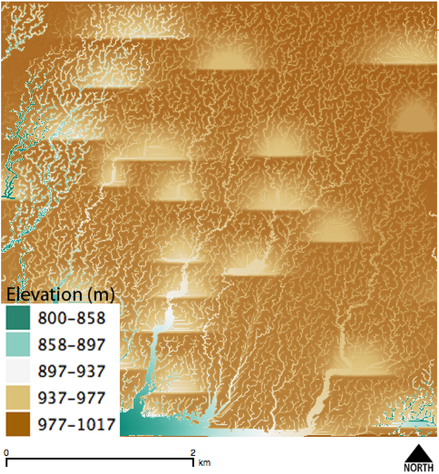
2.1. Synthetic Dataset

2.2. Real Dataset
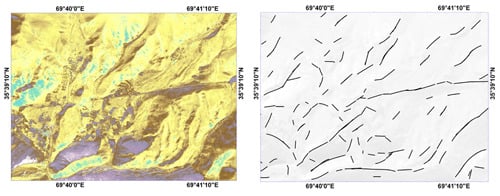
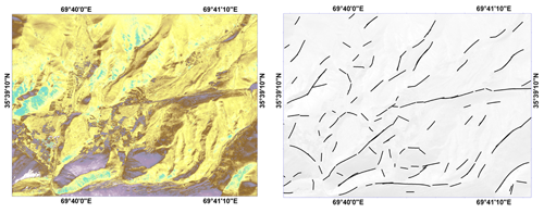
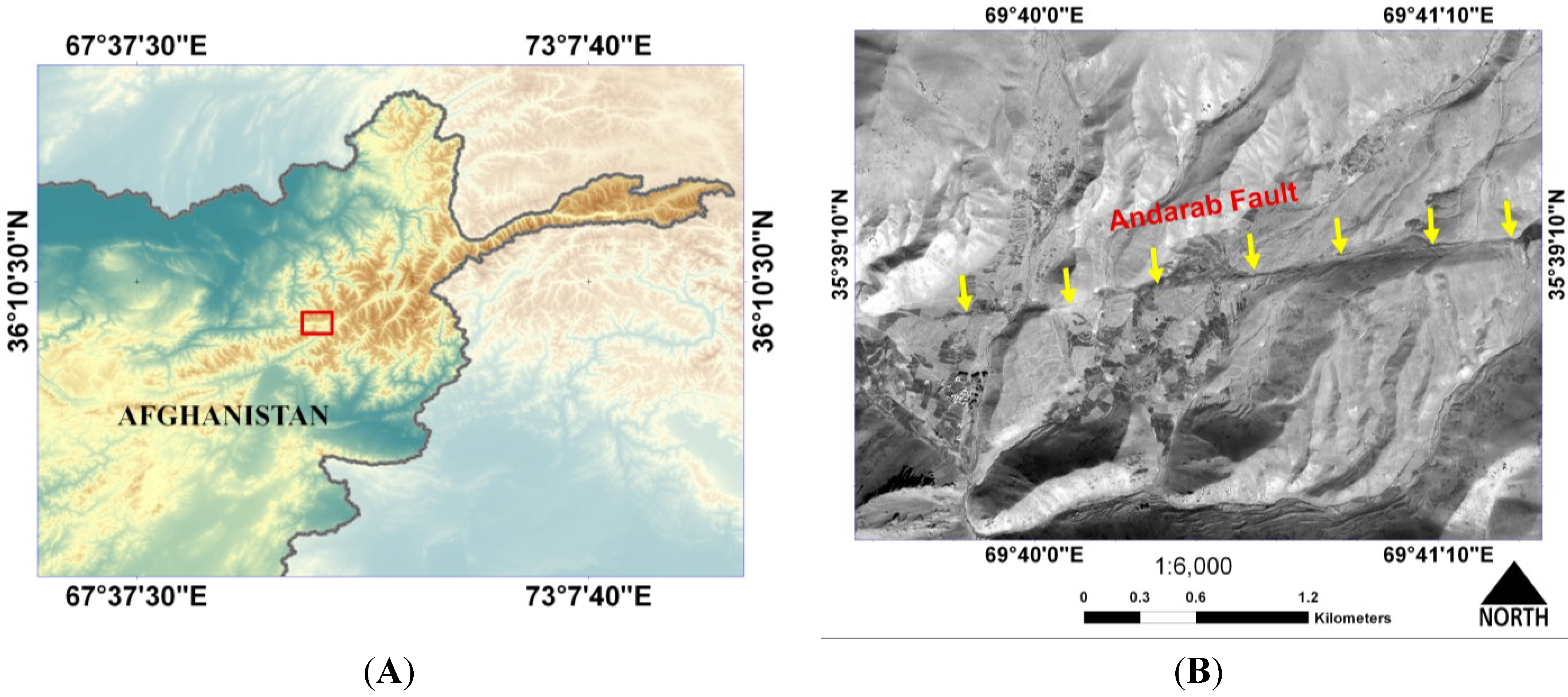
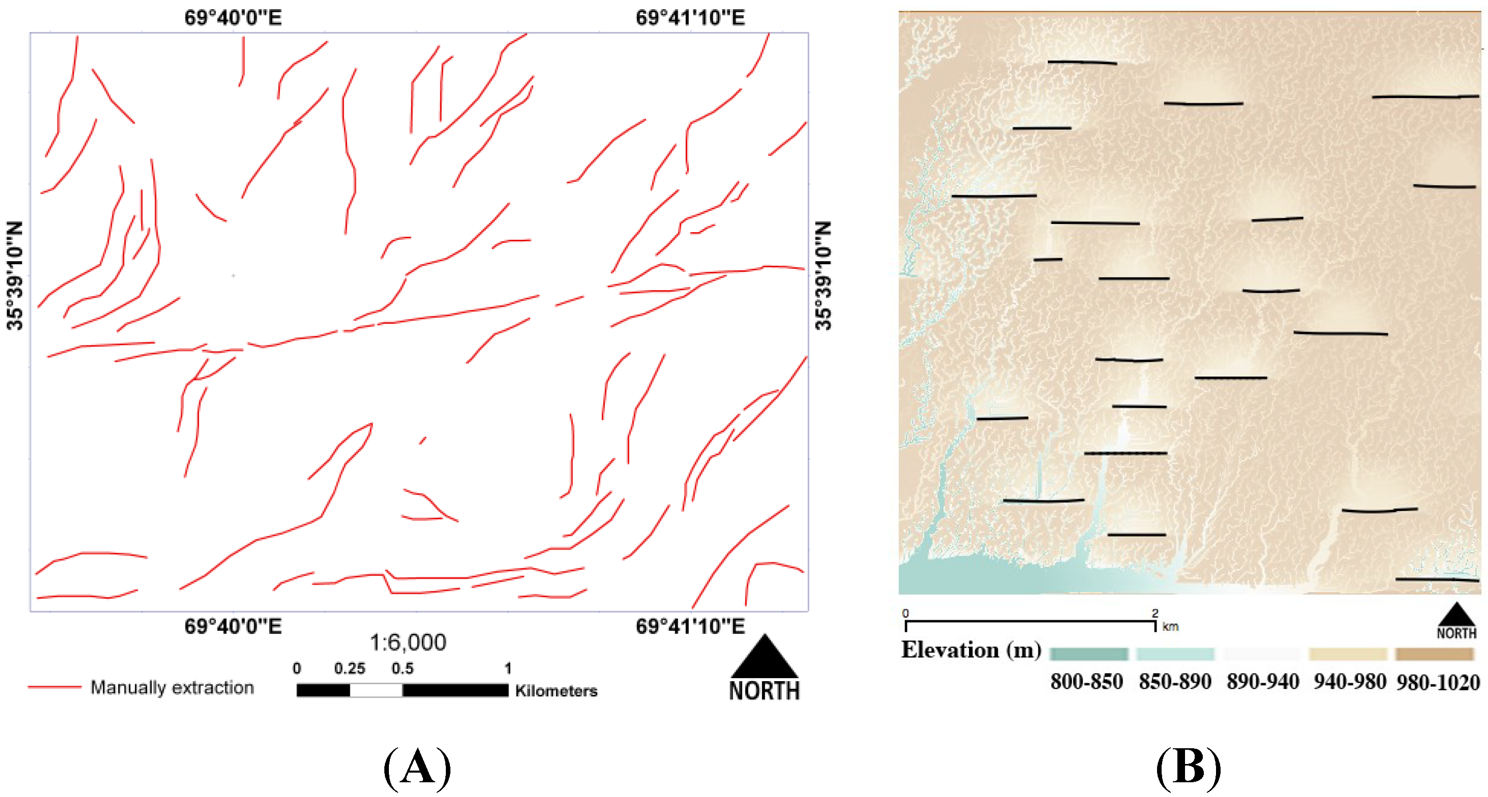
Study Area and Data

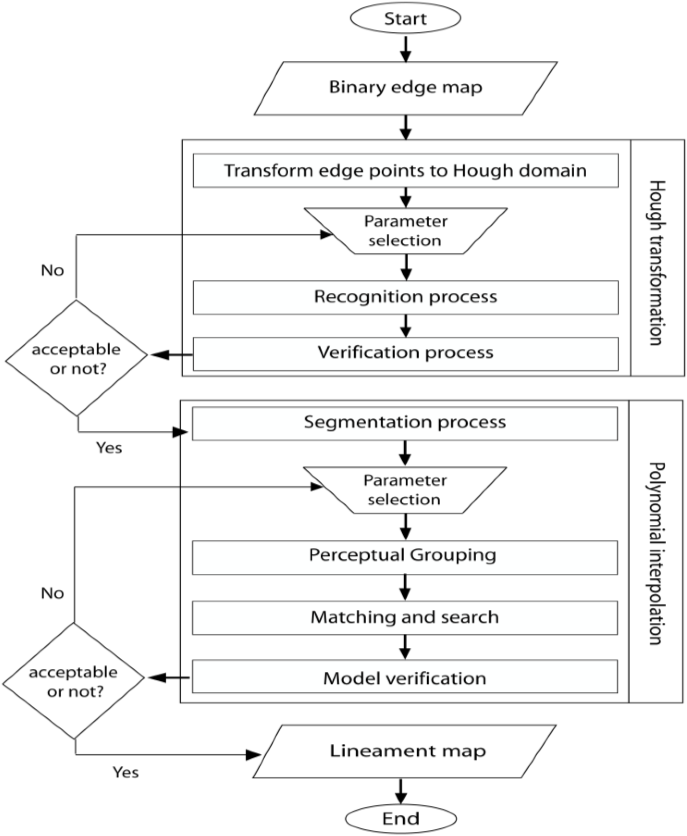
3. Methodology
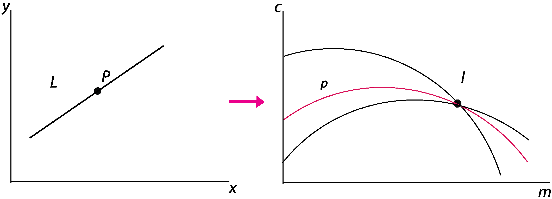
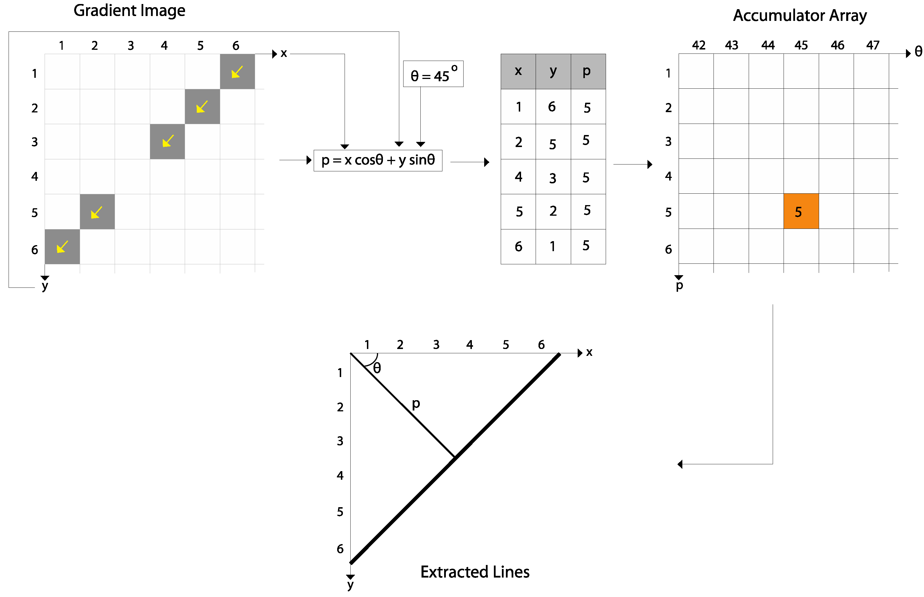
3.1. Hough Transform (HT)


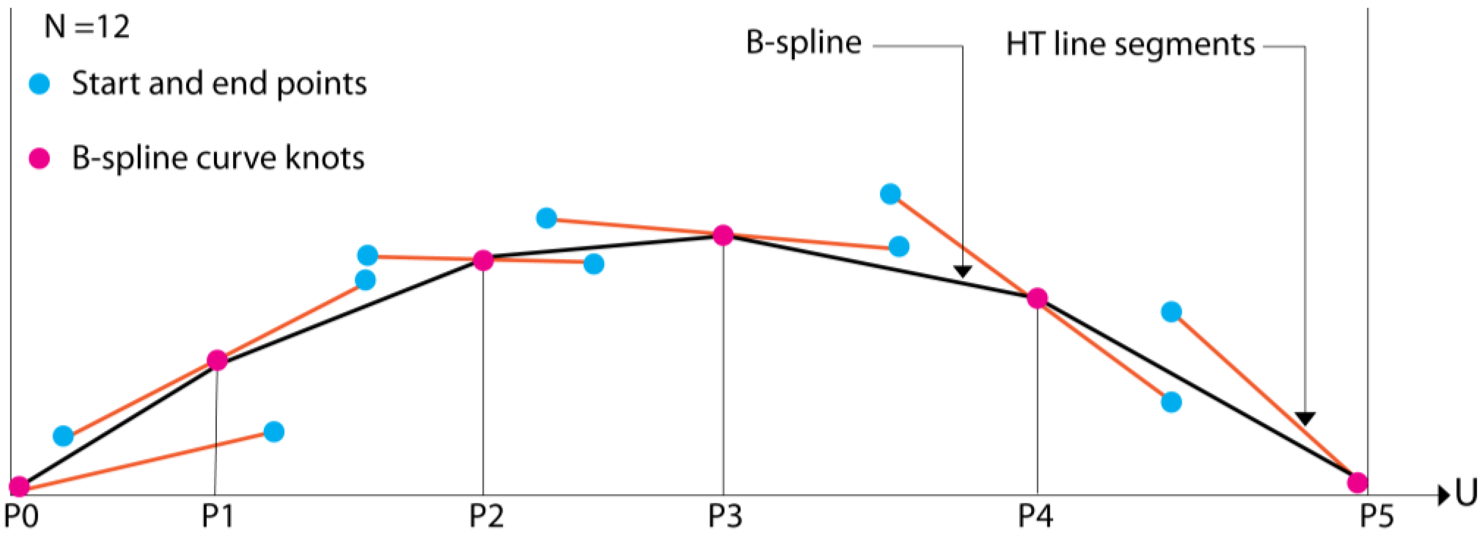
3.2. Grouping, Linking and Merging Line Segments
- (1)
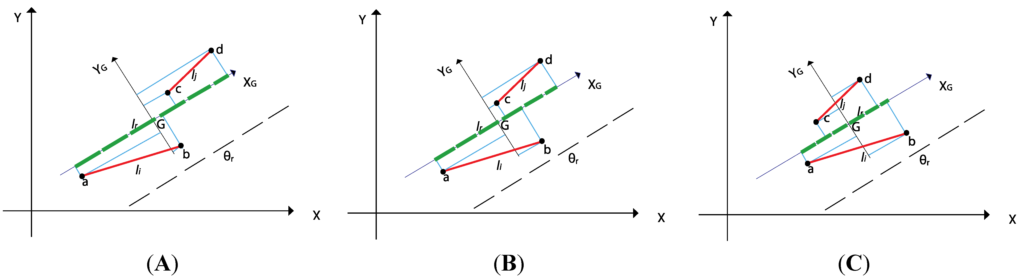
- Define point (, ) as a pair coordinates of the centroid by using the two segment endpoints (four points) and segment lengths:where a = (ax, ay) and b = (bx, by) are the endpoints of segment i, and c = (cx, cy) and d = (dx, dy) are the endpoints of segment j and are the lengths of segments i and j, respectively (Figure 6). The merged line will contain this centroid.Figure 6. (A) Merging of two non-overlapping, (B) partially overlapping and (C) totally overlapping segments by Tavares-Padilha method. The red segments are merged to the green lines.Figure 6. (A) Merging of two non-overlapping, (B) partially overlapping and (C) totally overlapping segments by Tavares-Padilha method. The red segments are merged to the green lines.
![Remotesensing 06 11468 g006]()
- (2)
- The orientation of the merged line (θr) is defined as the weighted sum of the orientations of the given segments. If thenelse
- (3)
- (XG, YG) coordinate system is defined on the centroid (xG, yG). The XG axis is parallel to the direction θr of the merged line.
- (4)
- Coordinates for the endpoints a, b, c and d of both segments in the (XG, YG) coordinate system are determined:where (, ) are the coordinates of the point δ in the (XG, YG) coordinate system. The endpoints coordinates in the new coordinate system are , = (, ), = (, ), = (, ) and = (, ).
- (5)
- The two orthogonal projections over the axis XG of the four endpoints a, b, c and d, which are farther apart, define the endpoints of the merged line [39].


3.3. Accuracy Measurements

4. Testing and Evaluating TecLines
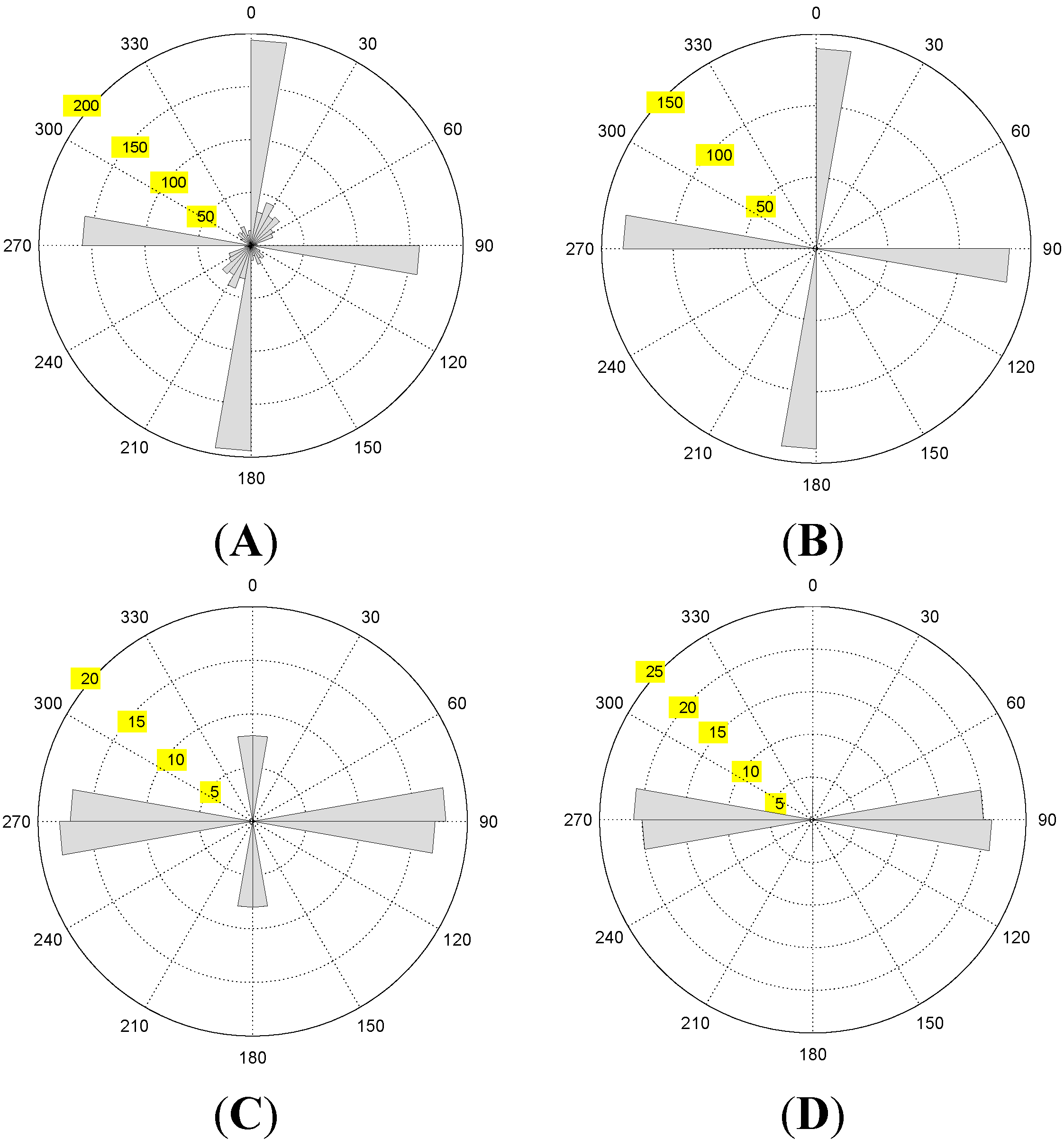
4.1. Performance Evaluation of the TecLines on a Synthetic Digital Elevation Model (DEM)

4.1.1. Qualitative Accuracy Assessment
4.1.2. Quantitative Accuracy Assessment


| Method | TP (m) | FP (m) | FN (m) | Length Accuracy (Matching Percentages) (%) | Overall Accuracy (%) |
|---|---|---|---|---|---|
| Hough Transform | 817 | 946 | 204 | 80 | 60 |
| Tavares-Padilha | 868 | 452 | 153 | 85 | 72 |
| B-spline | 970 | 223 | 51 | 95 | 90 |
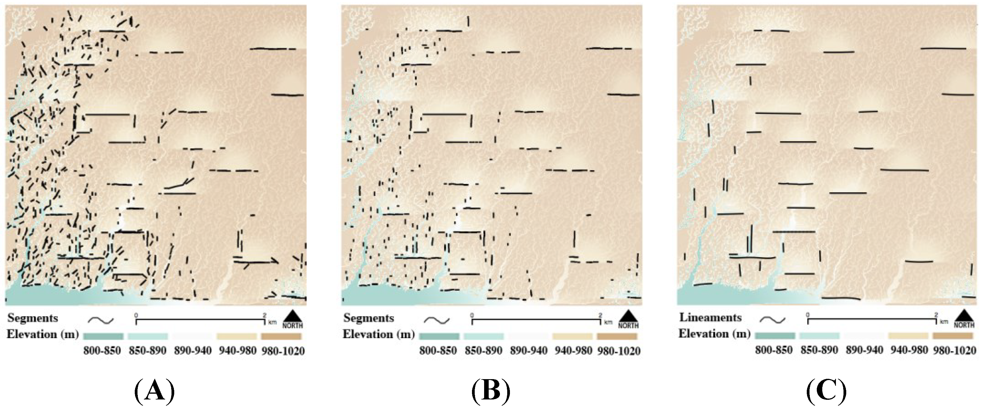
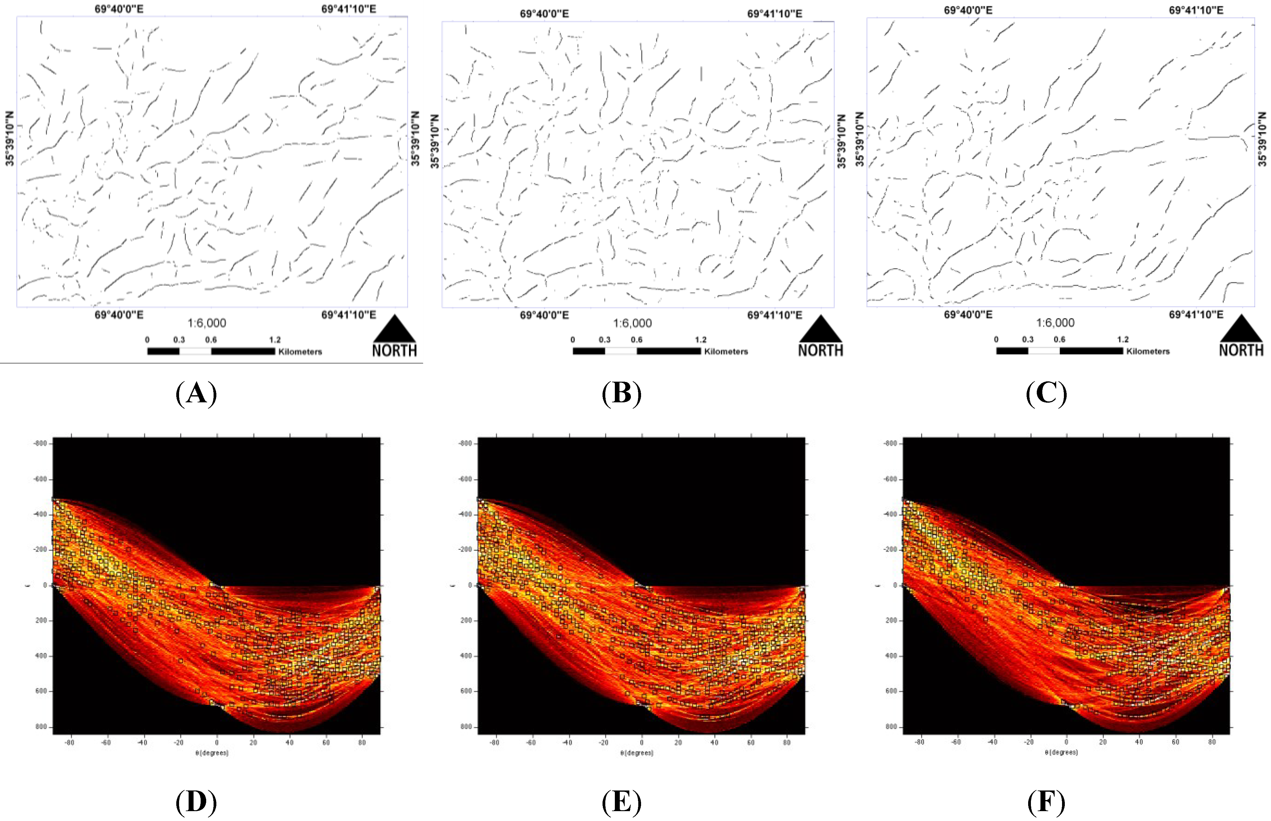
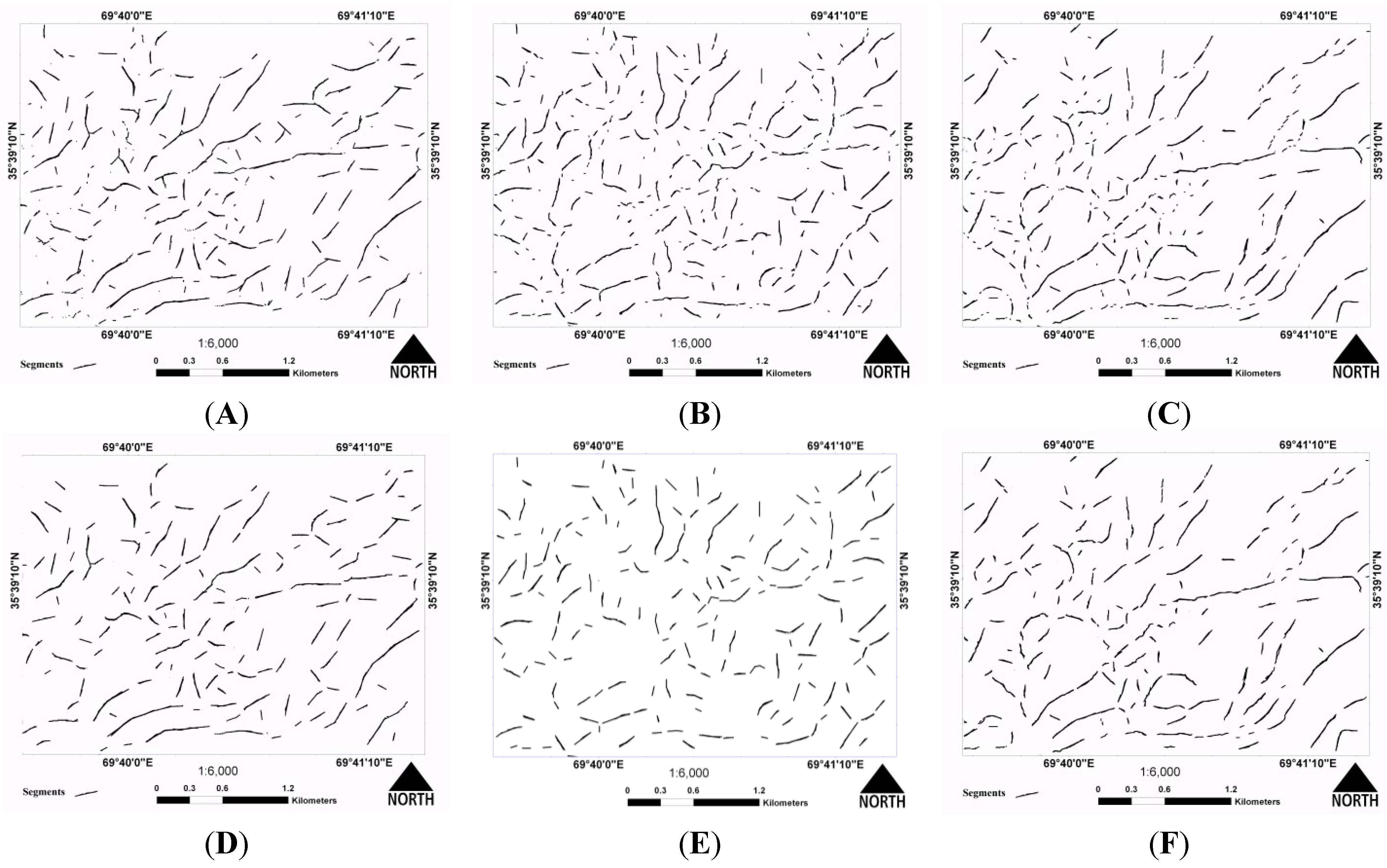
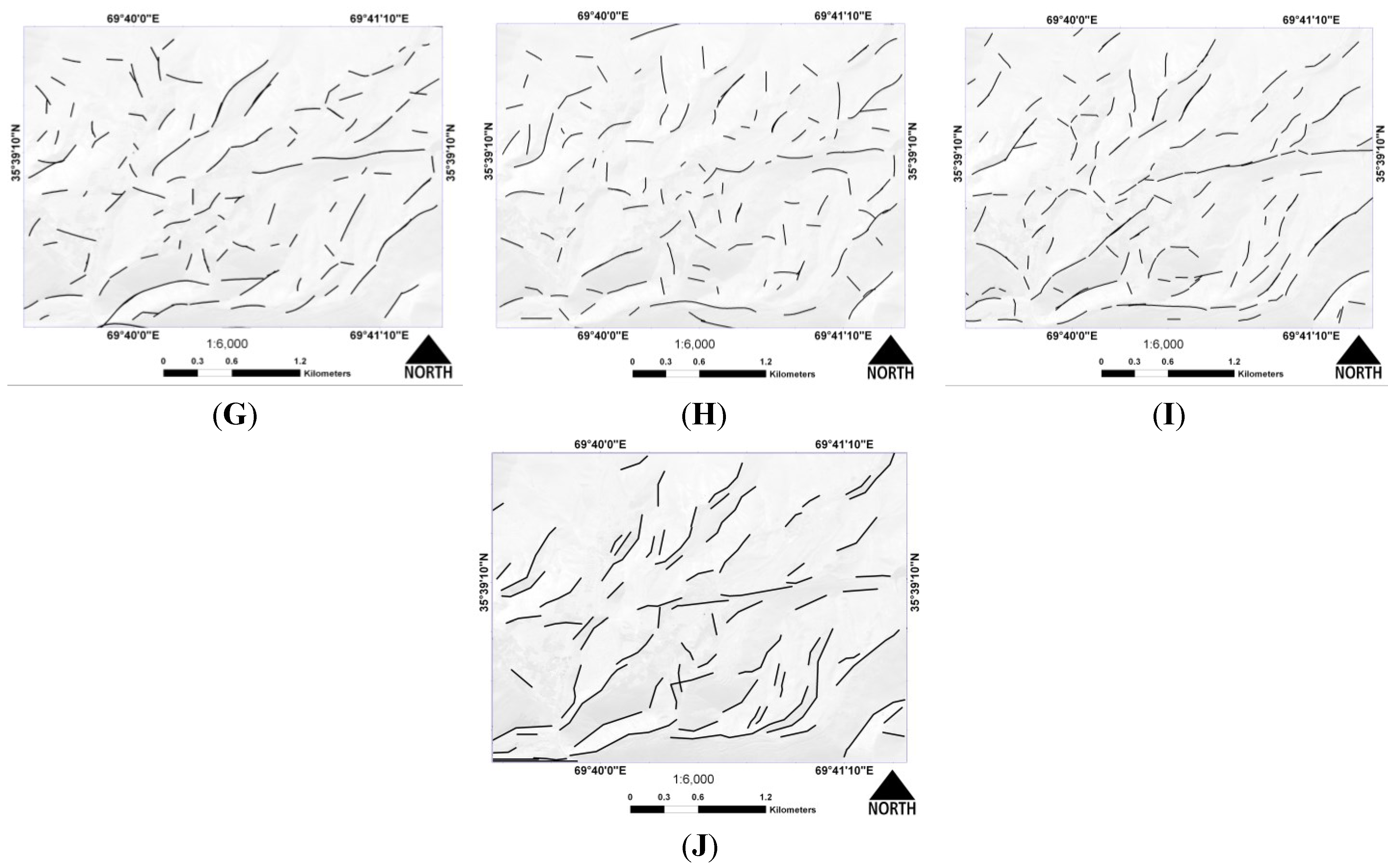
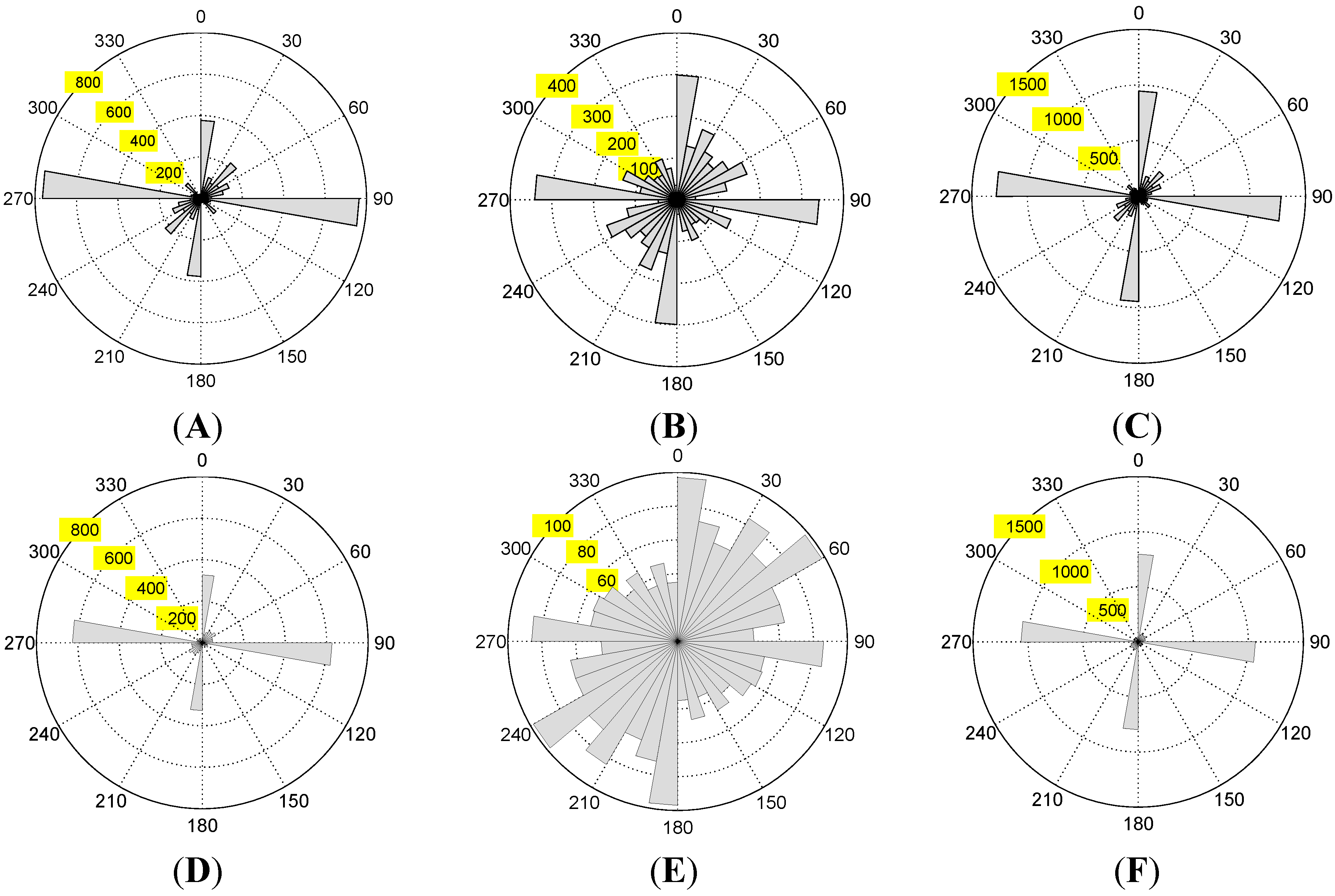
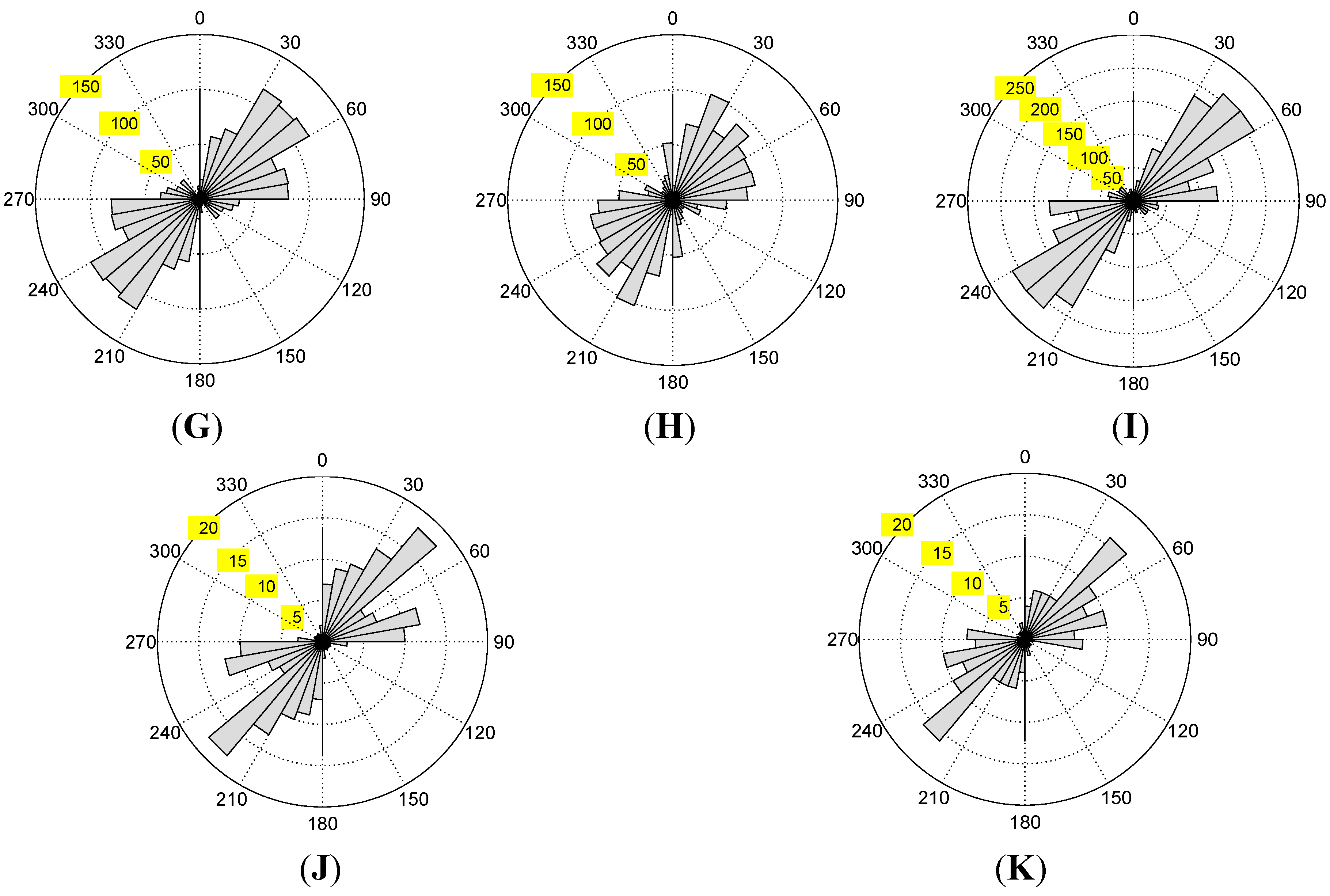
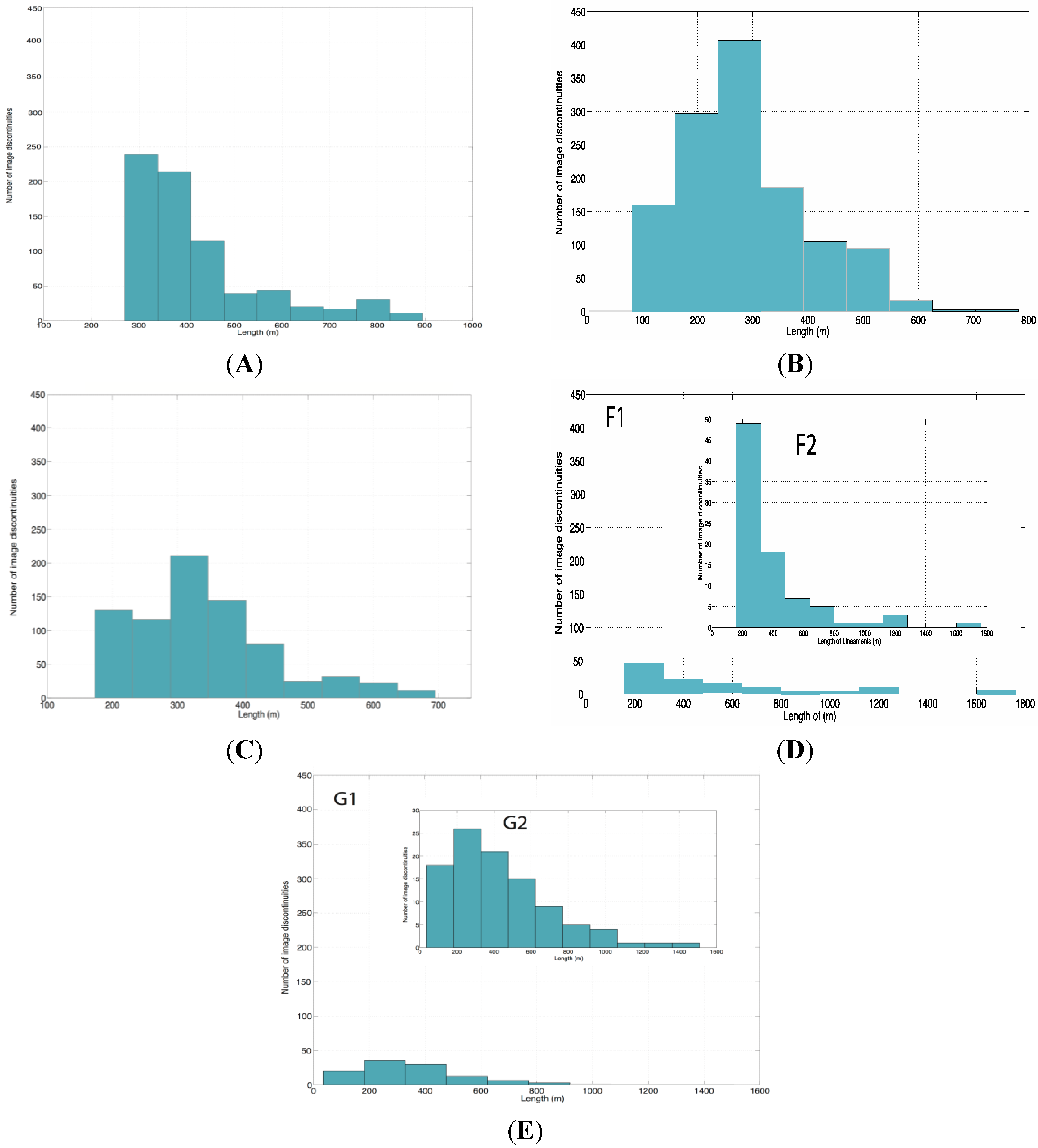
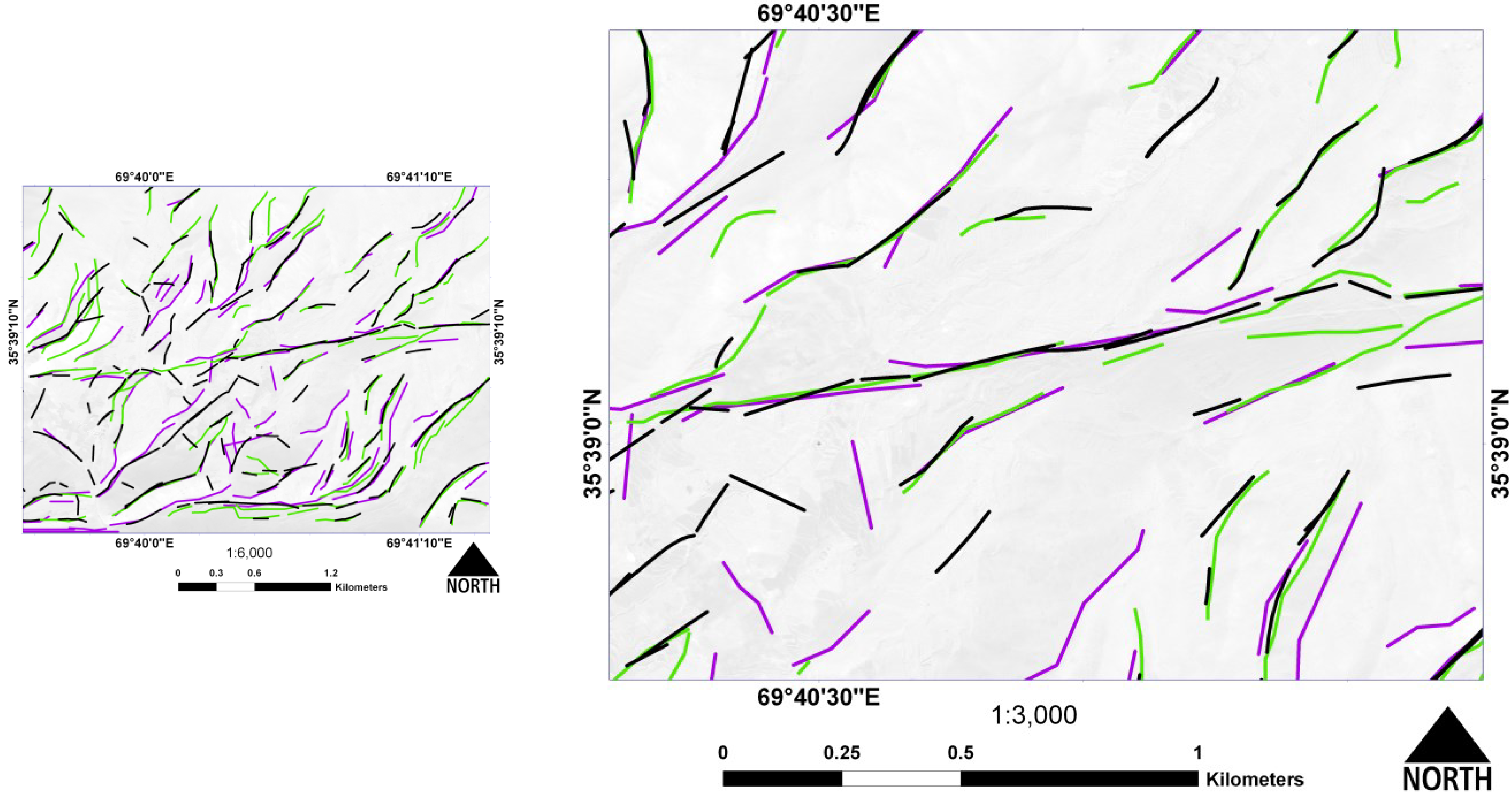
4.2. Experimental Results and Accuracy Assessment Using Real Dataset

| Parameters | TecLines Toolbox | Manually | PCI | ||||||||
|---|---|---|---|---|---|---|---|---|---|---|---|
| Hough Transform | Tavares-Padilha | B-Spline | |||||||||
| Sobel | LOG | Canny | Sobel | LOG | Canny | Sobel | LOG | Canny | |||
| Mean (m) | 32 | 35 | 22 | 98 | 89 | 96 | 392 | 320 | 288 | 433 | 379 |
| St deviation (m) | 45 | 31 | 30 | 112 | 97 | 105 | 145 | 120 | 113 | 275 | 285 |
| Sum (km) | 75 | 84 | 88 | 56 | 43 | 58 | 42 | 35 | 47 | 44 | 32 |
| Min (m) | 5 | 2 | 2 | 10 | 14 | 9 | 200 | 115 | 114 | 34 | 158 |
| Max (m) | 353 | 256 | 281 | 540 | 372 | 511 | 895 | 695 | 781 | 1508 | 1762 |
| Count | 2324 | 2362 | 4043 | 1481 | 1298 | 2725 | 892 | 875 | 1293 | 101 | 85 |
| Range (m) | 348 | 254 | 279 | 530 | 358 | 502 | 695 | 580 | 667 | 85 | 1604 |
| Median (m) | 11 | 23 | 10 | 180 | 134 | 173 | 365 | 319 | 275 | 12 | 271 |


4.2.1. Qualitative Accuracy Assessment
4.2.2. Quantitative Accuracy Assessment


| Method | TP (km) | FP (km) | FN (km) | Length Accuracy (Matching Percentages) (%) | Overall Accuracy (%) |
|---|---|---|---|---|---|
| Sobel | 31 | 11 | 13 | 70 | 62 |
| LOG | 27 | 8 | 17 | 61 | 56 |
| Canny | 36 | 9 | 8 | 81 | 73 |
| PCI | 32 | 6 | 12 | 72 | 67 |

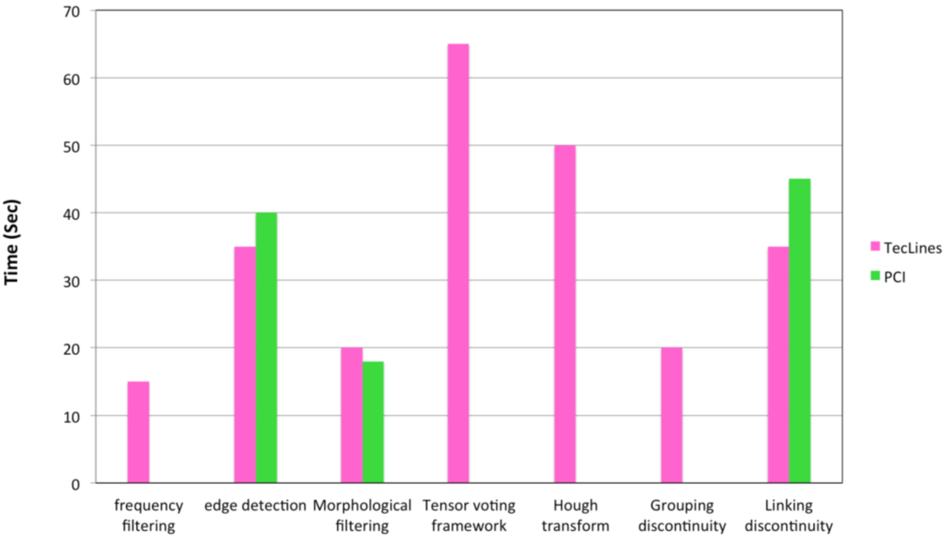
| Step | Time (Sec) | |
|---|---|---|
| TecLines (Canny) | PCI | |
| Frequency filtering | 15 | -- |
| Edge detection | 35 | 40 |
| Morphological filtering | 20 | 18 |
| Tensor voting framework | 65 | -- |
| Hough transform | 50 | -- |
| Grouping discontinuity | 20 | -- |
| Linking discontinuity | 35 | 45 |
5. Concluding Remarks
Acknowledgments
Author Contributions
Conflicts of Interest
References
- Raghavan, V.; Masumoto, S.; Koike, K.; Nagano, S. Automatic lineament extraction from digital images using a segment tracing and rotation transformation approach. Comput. Geosci. 1995, 21, 555–591. [Google Scholar]
- Chang, Y.-C.; Song, G.-S.; Hsu, S.-K. Automatic extraction of ridge and valley axes using the profile recognition and polygon-breaking algorithm. Comput. Geosci. 1998, 24, 83–93. [Google Scholar] [CrossRef]
- Vassilas, N.; Perantonis, S.; Charou, E.; Tsenoglou, T.; Stefouli, M.; Varoufakis, S. Delineation of lineaments from satellite data based on efficient neural network and pattern recognition techniques. In Proceedings of the 2nd Hellenic Conference on AI, SETN-2002, Thessaloniki, Greece, 11–12 April 2002.
- Wladis, D. Automatic lineament detection using digital elevation models with second derivative filters. Photogramm. Eng. Remote Sens. 1999, 65, 453–458. [Google Scholar]
- Comparison of Edge Detection and Hough Transform Techniques for the Extraction of Geologic Features. Available online: http://www.isprs.org/proceedings/XXXV/congress/comm3/papers/376.pdf (accessed on 13 November 2014).
- Fitton, N.C.; Cox, S.J.D. Optimising the application of the hough transform for automatic feature extraction from geoscientific images. Comput. Geosci. 1998, 24, 933–951. [Google Scholar] [CrossRef]
- Koike, K.; Nagano, S.; Kawaba, K. Construction and analysis of interpreted fracture planes through combination of satellite-image derived lineaments and digital elevation model data. Comput. Geosci. 1998, 24, 573–583. [Google Scholar] [CrossRef]
- Morris, K. Using knowledge-base rules to map the three-dimensional nature of geological features. Photogramm. Eng. Remote Sens. 1991, 57, 1209–1216. [Google Scholar]
- Suzen, M.L.; Toprak, V. Filtering of satellite images in geological lineament analyses: An application to a fault zone in central turkey. Int. J. Remote Sens. 1998, 19, 1101–1114. [Google Scholar] [CrossRef]
- Masoud, A.; Koike, K. Tectonic architecture through Landsat-7 ETM+/SRTM DEM-derived lineaments and relationship to the hydrogeologic setting in Siwa region, NW Egypt. J. Afr. Earth Sci. 2006, 45, 467–477. [Google Scholar] [CrossRef]
- Masoud, A.A.; Koike, K. Auto-detection and integration of tectonically significant lineaments from SRTM DEM and remotely-sensed geophysical data. ISPRS J. Photogramm. Remote Sens. 2011, 66, 818–832. [Google Scholar] [CrossRef]
- Tripathi, N.K.; Gokhale, K.; Siddiqui, M.U. Directional morphological image transforms for lineament extraction from remotely sensed images. Int. J. Remote Sens. 2000, 21, 3281–3292. [Google Scholar] [CrossRef]
- Zhang, L.; Wu, J.; Hao, T.; Wang, J. Automatic lineament extraction from potential-field images using the radon transform and gradient calculation. Geophysics 2006, 71, J31–J40. [Google Scholar] [CrossRef]
- Rahnama, M.; Gloaguen, R. Teclines: A matlab-based toolbox for tectonic lineament analysis from satellite images and dems, part 1: Line segment detection and extraction. Remote Sens. 2014, 6, 5938–5958. [Google Scholar] [CrossRef]
- Ghita, O.; Whelan, P.F. Computational approach for edge linking. J. Electronic Imaging 2002, 11, 479–485. [Google Scholar] [CrossRef]
- Sappa, A.D.; Vintimilla, B.X. Edge point linking by means of global and local schemes. In Signal Processing for Image Enhancement and Multimedia Processing; Springer: Berlin, Germany, 2008; pp. 115–125. [Google Scholar]
- Sinha, S.K.; Fieguth, P.W. Automated detection of cracks in buried concrete pipe images. Autom. Constr. 2006, 15, 58–72. [Google Scholar] [CrossRef]
- Cook, G.W.; Delp, E.J. Multiresolution sequential edge linking. In Proceedings of the International Conference on Image Processing 1995, Washington, DC, USA, 23–26 October 1995; pp. 41–44.
- Farag, A.A.; Delp, E.J. Edge linking by sequential search. Pattern Recognit. 1995, 28, 611–633. [Google Scholar] [CrossRef]
- Shih, F.Y.; Cheng, S. Adaptive mathematical morphology for edge linking. Inf. Sci. 2004, 167, 9–21. [Google Scholar] [CrossRef]
- Zhu, Q.; Payne, M.; Riordan, V. Edge linking by a directional potential function (DPF). Image Vis. Comput. 1996, 14, 59–70. [Google Scholar] [CrossRef]
- Palmer, P.L.; Kittler, J.; Petrou, M. Using focus of attention with the hough transform for accurate line parameter estimation. Pattern Recognit. 1994, 27, 1127–1134. [Google Scholar] [CrossRef]
- Matas, J.; Galambos, C.; Kittler, J. Robust detection of lines using the progressive probabilistic hough transform. Comput. Vis. Image Underst. 2000, 78, 119–137. [Google Scholar] [CrossRef]
- Yang, K.; Sam Ge, S.; He, H. Robust line detection using two-orthogonal direction image scanning. Comput. Vis. Image Underst. 2011, 115, 1207–1222. [Google Scholar] [CrossRef]
- Yip, R.K.K.; Lam, W.C.Y.; Tam, P.K.S.; Leung, D.N.K. A hough transform technique for the detection of rotational symmetry. Pattern Recognit. Lett. 1994, 15, 919–928. [Google Scholar] [CrossRef]
- Duda, R.O.; Hart, P.E. Use of the hough transformation to detect lines and curves in pictures. Commun. ACM 1972, 15, 11–15. [Google Scholar] [CrossRef]
- Palmer, P.L.; Kittler, J.; Petrou, M. An optimizing line finder using a hough transform algorithm. Comput. Vis. Image Underst. 1997, 67, 1–23. [Google Scholar] [CrossRef]
- Hough, P.V.C. Method and Means for Recognizing Complex Patterns. U.S. Patents 3069654 A, 18 December 1962. [Google Scholar]
- Duda, R.O.; Hart, P.E. Pattern Recognation and Scene Analysis; Wiley: New York, NY, USA, 1973; Volume 3. [Google Scholar]
- Illingworth, J.; Kittler, J. A survey of the hough transform. Comput. Vis. Graph. Image Process. 1988, 44, 87–116. [Google Scholar] [CrossRef]
- Kiryati, N.; Eldar, Y.; Bruckstein, A.M. A probabilistic hough transform. Pattern Recognit. 1991, 24, 303–316. [Google Scholar] [CrossRef]
- Cross, A.; Wadge, G. Geological lineament detection using the hough transform. In Remote Sensing: Moving Towards the 21st Century; The National Aeronautics and Space Administration (NASA): Washington, DC, USA, 1988; pp. 1779–1782. [Google Scholar]
- Wadge, G.; Cross, A. Quantitative methods for detecting aligned points: An application to the volcanic vents of the michoacan-guanajuato volcanic field, Mexico. Geology 1988, 16, 815–818. [Google Scholar] [CrossRef]
- Wang, J.; Howarth, P.J. Use of the hough transform in automated lineament. IEEE Trans. Geosci. Remote Sens. 1990, 28, 561–567. [Google Scholar] [CrossRef]
- Van der Werff, H.M.A.; Bakker, W.H.; van der Meer, F.D.; Siderius, W. Combining spectral signals and spatial patterns using multiple hough transforms: An application for detection of natural gas seepages. Comput. Geosci. 2006, 32, 1334–1343. [Google Scholar]
- Karnieli, A.; Meisels, A.; Fisher, L.; Arkin, Y. Automatic extraction and evaluation of geological linear features from digital remote sensing data using a hough transform. Photogramm. Eng. Remote Sens. 1996, 62, 525–531. [Google Scholar]
- Fernandes, L.A.F.; Oliveira, M.M. Real-time line detection through an improved hough transform voting scheme. Pattern Recognit. 2008, 41, 299–314. [Google Scholar] [CrossRef]
- Samal, A.; Edwards, J. Generalized hough transform for natural shapes. Pattern Recognit. Lett. 1997, 18, 473–480. [Google Scholar] [CrossRef]
- A New Approach for Merging Edge Line Segments. Available online: http://repositorio-aberto.up.pt/bitstream/10216/420/2/27110.pdf (accessed on 13 November 2014).
- Hussien, B.; Sridhar, B. Robust line extraction and matching algorithm. Proc. SPIE 1993, 2055. [Google Scholar] [CrossRef]
- Prautzsch, H.; Boehm, W.; Paluszny, M. Bézier and b-Spline Techniques; Springer: Berlin, Germany, 2002. [Google Scholar]
- Ziou, D.; Koukam, A. Knowledge-based assistant for the selection of edge detectors. Pattern Recognit. 1998, 31, 587–596. [Google Scholar] [CrossRef]
- Nguyen, T.B.; Ziou, D. Contextual and non-contextual performance evaluation of edge detectors. Pattern Recognit. Lett. 2000, 21, 805–816. [Google Scholar] [CrossRef]
- Heath, M.D.; Sarkar, S.; Sanocki, T.; Bowyer, K.W. A robust visual method for assessing the relative performance of edge-detection algorithms. IEEE Trans. Pattern Anal. Mach. Intell. 1997, 19, 1338–1359. [Google Scholar] [CrossRef]
- Cho, K.; Meer, P.; Cabrera, J. Performance assessment through bootstrap. IEEE Trans. Pattern Anal. Mach. Intell. 1997, 19, 1185–1198. [Google Scholar] [CrossRef]
- Lopez-Molina, C.; de Baets, B.; Bustince, H. Quantitative error measures for edge detection. Pattern Recognit. 2013, 46, 1125–1139. [Google Scholar] [CrossRef]
- Ji, Q.; Haralick, R.M. Efficient facet edge detection and quantitative performance evaluation. Pattern Recognit. 2002, 35, 689–700. [Google Scholar]
- Román-Roldán, R.; Gómez-Lopera, J.F.; Atae-Allah, C.; Martı́nez-Aroza, J.; Luque-Escamilla, P.L. A measure of quality for evaluating methods of segmentation and edge detection. Pattern Recognit. 2001, 34, 969–980. [Google Scholar]
- Salotti, M.; Bellet, F.; Garbay, C. Evaluation of Edge Detectors: Critics and Proposal; CiteSeer, The Pennsylvania State University: Pennsylvania, PA, USA, 1996. [Google Scholar]
- Kim, D.-S.; Lee, W.-H.; Kweon, I.-S. Automatic edge detection using 3 × 3 ideal binary pixel patterns and fuzzy-based edge thresholding. Pattern Recognit. Lett. 2004, 25, 101–106. [Google Scholar] [CrossRef]
- Nezamabadi-pour, H.; Saryazdi, S.; Rashedi, E. Edge detection using ant algorithms. Soft Comput. 2006, 10, 623–628. [Google Scholar] [CrossRef]
- Chang, K.; Bowyer, K.W.; Sarkar, S.; Victor, B. Comparison and combination of ear and face images in appearance-based biometrics. IEEE Trans. Pattern Anal. Mach. Intell. 2003, 25, 1160–1165. [Google Scholar] [CrossRef]
- Shin, M.C.; Goldgof, D.B.; Bowyer, K.W. Comparison of edge detector performance through use in an object recognition task. Comput. Vis. Image Underst. 2001, 84, 160–178. [Google Scholar] [CrossRef]
- Heath, M.; Sarkar, S.; Sanocki, T.; Bowyer, K. Comparison of edge detectors: A methodology and initial study. In Proceedings of the 1996 IEEE Computer Society Conference on Computer Vision and Pattern Recognition, 1996, CVPR’96, San Francisco, CA, USA, 18–20 June 1996; pp. 143–148.
- Pellegrino, F.A.; Vanzella, W.; Torre, V. Edge detection revisited. IEEE Trans. Syst. Man Cybern. Part B 2004, 34, 1500–1518. [Google Scholar] [CrossRef]
- Yitzhaky, Y.; Peli, E. A method for objective edge detection evaluation and detector parameter selection. IEEE Trans. Pattern Anal. Mach. Intell. 2003, 25, 1027–1033. [Google Scholar] [CrossRef]
- Schroeder, S.; Babeyko, A.Y. Implementation of large-scale landscape evolution modelling to real high-resolution DEM. In Proceedings of the AGU Fall Meeting, San Francisco, NC, USA, 3–7 December 2012; p. 2677.
- Map and Database of Probable and Possible Quaternary Faults in Afghanistan. Available online: http://pubs.usgs.gov/of/2007/1103/ (accessed on 13 November 2014).
- Wheeler, R.L.; Bufe, C.G.; Johnson, M.L.; Dart, R.L. Seismotectonic Map of Afghanistan, with Annotated Bibliography; US Department of the Interior, US Geological Survey: Reston, VA, USA, 2005. [Google Scholar]
- Ambraseys, N.; Bilham, R. The tectonic setting of bamiyan and the seismicity in and near afghanistan for the past 12 centuries. In After the Destruction of the Giant Buddha Statues in Bamiyan (Afghanistan) in 2001; Margottini, C., Ed.; Springer Berlin Heidelberg: Berlin, Germany, 2009; pp. 67–94. [Google Scholar]
- Molnar, P.; Tapponnier, P. Relation of the tectonics of eastern China to the India-Eurasia collision: Application of slip-line field theory to large-scale continental tectonics. Geology 1977, 5, 212–216. [Google Scholar] [CrossRef]
- Wellman, H.W. Active wrench faults of Iran, Afghanistan and Pakistan. Geol. Rundsch. 1966, 55, 716–735. [Google Scholar] [CrossRef]
- Ai, J.; Qi, X.; Yu, W.; Deng, Y.; Liu, F.; Shi, L.; Jia, Y. A novel ship wake cfar detection algorithm based on scr enhancement and normalized hough transform. IEEE Trans. Geosci. Remote Sens. Lett. 2011, 8, 681–685. [Google Scholar] [CrossRef]
- Chong, J.-S.; Zhu, M.-H. Ship wake detection algorithm in SAR image based on normalized grey level Hough transform. J. Image Graphics 2004, 9, 146–150. [Google Scholar]
- Lu, D.-S.; Chen, C.-C. Edge detection improvement by ant colony optimization. Pattern Recognit. Lett. 2008, 29, 416–425. [Google Scholar] [CrossRef]
- Manish, T.I.; Murugan, D.; Kumar, G. Hybrid edge detection using canny and ant colony optimization. Commun. Inf. Sci. Manag. Eng. 2013, 3, 402–405. [Google Scholar]
- PCI. Geomatica Version 10.3 Users Manual; PCI Geomatics Enterprises: Richmond Hill, ON, Canada, 2009. [Google Scholar]
- Tectonic Lineament Analysis Using Remote Sensing Datasets Tollbox (Teclines). http://www.teclines.net (accessed on 5 November 2014).
© 2014 by the authors; licensee MDPI, Basel, Switzerland. This article is an open access article distributed under the terms and conditions of the Creative Commons Attribution license (http://creativecommons.org/licenses/by/4.0/).
Share and Cite
Rahnama, M.; Gloaguen, R. TecLines: A MATLAB-Based Toolbox for Tectonic Lineament Analysis from Satellite Images and DEMs, Part 2: Line Segments Linking and Merging. Remote Sens. 2014, 6, 11468-11493. https://doi.org/10.3390/rs61111468
Rahnama M, Gloaguen R. TecLines: A MATLAB-Based Toolbox for Tectonic Lineament Analysis from Satellite Images and DEMs, Part 2: Line Segments Linking and Merging. Remote Sensing. 2014; 6(11):11468-11493. https://doi.org/10.3390/rs61111468
Chicago/Turabian StyleRahnama, Mehdi, and Richard Gloaguen. 2014. "TecLines: A MATLAB-Based Toolbox for Tectonic Lineament Analysis from Satellite Images and DEMs, Part 2: Line Segments Linking and Merging" Remote Sensing 6, no. 11: 11468-11493. https://doi.org/10.3390/rs61111468