Detecting Landscape Changes in High Latitude Environments Using Landsat Trend Analysis: 2. Classification

Abstract

Mapping landscape dynamics is necessary to assess cumulative impacts due to climate change and development in Arctic regions. Landscape changes produce a range of temporal reflectance trajectories that can be obtained from remote sensing image time-series. Mapping these changes assumes that their trajectories are unique and can be characterized by magnitude and shape. A companion paper in this issue describes a trajectory visualization method for assessing a range of landscape disturbances. This paper focusses on generating a change map using a time-series of calibrated Landsat Tasseled Cap indices from 1985 to 2011. A reference change database covering the Mackenzie Delta region was created using a number of ancillary datasets to delineate polygons describing 21 natural and human-induced disturbances. Two approaches were tested to classify the Landsat time-series and generate change maps. The first involved profile matching based on trajectory shape and distance, while the second quantified profile shape with regression coefficients that were input to a decision tree classifier. Results indicate that classification of robust linear trend coefficients performed best. A final change map was assessed using bootstrapping and cross-validation, producing an overall accuracy of 82.8% at the level of 21 change classes and 87.3% when collapsed to eight underlying change processes.

1. Introduction

Earth observation involves predicting the state and change of the earth’s surface. Land cover and biophysical parameter mapping predict the state of the surface within each ground element represented by an image pixel. Change detection records alterations of ground element states in time that can be broadly grouped as either abrupt or gradual. Abrupt change refers to a rapid state change of the pixel usually within an observation period of one year and includes disturbances such as fire, and land use conversions such as urban expansion. Gradual change involves processes that occur over a period of several years and includes vegetation regeneration, dieback, succession and arctic greening caused by climate warming [1].

A common goal of change detection is the creation of a map time-series [2]. In this case, change detection is applied to map a land cover conversion from an initial state to a changed state (i.e., from-to conversion). The process causing the state change is inferred by the land cover class before and after change. For example, a forest pixel that becomes charred/barren suggests forest fire as the agent of change. Over a period of a decade or more, that same pixel transitions to herbaceous and then shrub, and the process inferred by this gradual conversion is regeneration. Notable exceptions to this common application of change detection are where change agents or processes are mapped directly. Such applications include fire mapping [3] and arctic greening. In the case of greening, the process of increasing arctic vegetation is commonly inferred by trend detection applied to NDVI time-series [4].

This paper presents research towards the development of a change product for northern cumulative impact assessment using Landsat image time-series covering the lower Mackenzie River and Delta region. The goal was to map processes or agents of change in the region rather than create a land cover time-series. Common change agents in the region include natural and human disturbances, as well as climate warming that is altering permafrost, hydrology, and vegetation. Changes can be broadly grouped into processes such as fire, regeneration, vegetation colonization, greening, vegetation removal, erosion and deposition/drainage. Each process can only occur in certain environments or geographical context such forest, tundra, lakes, rivers, or coastlines, which helps further specify the nature of change.

Fraser et al. [5] describe the major types of landscape changes included in the reference disturbance database used in the current study, as well as provide a legend for visually interpreting Landsat Tasseled Cap linear trends displayed as an R-G-B composite. That study alludes to the potential to classify Landsat Tasseled Cap trend images in Arctic environments to generate change maps. This study builds on Fraser et al. [5] by testing different methods to generate a change map, apply best methods and perform a proper assessment of the final map product.

Change mapping is performed by classifying each pixel’s trajectory in the three dimensions of Landsat data that include Tasseled Cap Brightness, Wetness and Greenness indices [6] contained in a Landsat time-series image stack. Classification is tested using two different approaches. First, a reference change trajectory database is created and template matching algorithms based on distance and shape are applied to determine a best-fit change class on a pixel basis. Second, trends are computed on a pixel basis and trend coefficients are input into a decision tree classifier to predict change class. Linear least-squares, Thiel-Sen robust linear and second and third-order polynomial trend coefficients are tested. Previous work alludes to the potential of profile matching for forest fire disturbance mapping and recovery, while this paper is the first to our knowledge to test similar approaches in Arctic environments [7,8,9].

Study Area

The study area includes the Tuktoyaktuk Coastal Plain and extends south across the Mackenzie Delta to the Richardson Mountains and then southeast to near Fort Good Hope (Figure 1). The region is entirely underlain by continuous permafrost [10] with 10% or more ice content, creating landforms characteristic of periglacial environments such as ice wedge polygons, thaw slumps and pingos [11]. Shallow lakes and ponds are widespread in the Delta and along the Tuktoyaktuk Peninsula where surficial geology consists mainly of colluvial, alluvial and lacustrine deposits. Lakes generally become larger and less numerous [12] to the south, where surficial geology consists mainly of till veneer and till blanket.

Figure 1. Study area covered by Landsat image stack from 1985 to 2011. Region 2 (R2) provided training data while Region 1 (R1) and Region 3 (R3) were used for validation.

Figure 1. Study area covered by Landsat image stack from 1985 to 2011. Region 2 (R2) provided training data while Region 1 (R1) and Region 3 (R3) were used for validation.

Vegetation transitions from forest to tundra across treeline that extends east-west just south of the Tuktoyaktuk Peninsula, reaching the Beaufort Sea in the Mackenzie Delta [13]. Above treeline, vegetation is nearly continuous and consists mainly of erect shrubs (Betula spp., Salix spp., Alnus spp.), dwarf shrubs and heath shrubs (Dryas spp., Empetrum spp., Ledum spp., Vaccinuim spp., Arctostaphylos spp.), cotton-grass tundra (Eriphorum spp., Carex spp.) and non-vascular lichen and moss species (Cladonia spp, Cladina spp., Sphagnum spp.) on polygons. White spruce (Picea glauca) is the dominant tree species at treeline. Fire is a common stand-replacing disturbance as indicated by numerous large fire scars south of treeline, while less frequent and smaller scars occur within tundra.

Mean winter temperature was approximately −25 degrees C from 1985 to 2012 and varies little north to south according to Environment Canada’s Homogenized temperature data for Tuktoyaktuk (Latitude: 69.43 degrees), Inuvik (Latitude: 68.3 degrees) and Fort Good Hope, NWT (Latitude: 66.24 degrees) [14]. The western Arctic of North America has experienced some of the most rapid climate warming on earth over the last 40 years [15]. At Inuvik where the climate record is most complete over the period of analysis, winter temperatures have increased more than summer temperatures since 1985 (0.14 degrees C summer; 4.06 degrees C winter) (Figure 2).

Figure 2. Inuvik summer (June–August) and winter (December–February) temperature trends from 1985 to 2011.

Figure 2. Inuvik summer (June–August) and winter (December–February) temperature trends from 1985 to 2011.

2. Data

2.1. Landsat

122 Landsat 5 (TM) and 7 (ETM+) images were obtained from the USGS Glovis data archive representing years from 1985 to 2011, and WRS Paths 59 to 64 and Rows 11 to 13. Images were selected to be as close to mid-summer as possible with anniversary dates ranging from 26 June to 27 August. Image stacks were processed in three separate regions due to their size with Region 1 covering the most of the Tuktoyaktuk Peninsula, Region 2 spanning the Mackenzie Delta north to south and Region 3 extending approximately 125 km south of the Delta near Fort Good Hope (Figure 1). Scenes were screened to remove cloud and cloud shadow and converted to Top-of-Atmosphere reflectance [16]. Calibration to surface reflectance was not performed since we assumed no systematic trends in aerosol optical depth, while random atmospheric effects were to be removed by trend detection. Landsat TOA Tasseled Cap Brightness, Wetness and Greenness Indices [6] were computed for each scene and index images were stacked to form cubes with dimensions x and y representing space and dimension z representing time. Certain scenes were imaged twice in one year and time was represented as number of days since the first image in the stack. Certain Path/Rows were common between regions while others were unique to individual regions. In addition, there is large overlap of WRS-2 Landsat frames at high latitudes. Thus, each region contained a variable number of temporal observations depending on scenes, scene overlap and missing data due to cloud, cloud shadow and Scan Line Correction (SLC) failure of Landsat 7 post-2003.

Table 1. Reference data used to identify and corroborate landscape changes observable in the Landsat trend imagery.

Data Set	Description	Types of Change Features Corroborated
Mackenzie Valley Orthophotos (MVAP)	Contracted by Indian and Northern Affairs Canada, photos are from August 2004, 1:3000 scale, ~1 m resolution	Slumps, drained lakes, seismic lines
NWT Community Orthophotos	Acquired by NWT Department of Municipal and Community Affairs in 2007–2012, 5 cm resolution.	Footprint and type of municipal development
SPOT Imagery	2005–2010 SPOT 4&5 imagery processed by NWT Centre for Geomatics, pan-fused 10 m resolution	All
Landsat TM and ETM+ imagery	Visual interpretation of 1985 and 2011 image pairs used to generate image stacks	All
Fire History of NWT	NWT Department of Environment and Natural Resources, 1965–2011 burned area polygons	Post-1965 forest fires
National Air Photo Library photographs	Panchromatic photographs 1950–1985, scales of 1:5000+	Pre-1965 forest and tundra fires, thaw slump progression
Ecological Land Classification (ELC) oblique air photos	NWT Department of Environment and Natural Resources, >60,000 oblique aerial photographs from 2005 to 2009.	All
Vertical color and color-infrared air photo pairs	208 vertical air photos pairs from 1980 and 2013, ~2–4 cm effective resolution, 14 flight lines over Tuktoyaktuk Peninsula [16]	Shrub proliferation
Oblique air photos from helicopter	Photos taken around Ft McPherson and between Inuvik and Tuk, August 2013, and around Yellowknife, August 2011 and June 2012.	All
Google Earth	Areas containing high resolution (<4 m) imagery	All
National Hydro Network	Lake perimeters and stream networks at 1:50,000 scale	Draining lakes, thaw slumps
Peel Plateau thaw slumps	212 digitized slumps [17]	Retrogressive thaw slumps
NWT Seismic Lines	Historical seismic line GIS database from National Energy Board	Seismic line disturbances
NWT Spatial Data Warehouse	Geospatial Portal containing numerous NWT spatial datasets	Mineral, oil, and gas developments

Table 1. Reference data used to identify and corroborate landscape changes observable in the Landsat trend imagery.

Data Set	Description	Types of Change Features Corroborated
Mackenzie Valley Orthophotos (MVAP)	Contracted by Indian and Northern Affairs Canada, photos are from August 2004, 1:3000 scale, ~1 m resolution	Slumps, drained lakes, seismic lines
NWT Community Orthophotos	Acquired by NWT Department of Municipal and Community Affairs in 2007–2012, 5 cm resolution.	Footprint and type of municipal development
SPOT Imagery	2005–2010 SPOT 4&5 imagery processed by NWT Centre for Geomatics, pan-fused 10 m resolution	All
Landsat TM and ETM+ imagery	Visual interpretation of 1985 and 2011 image pairs used to generate image stacks	All
Fire History of NWT	NWT Department of Environment and Natural Resources, 1965–2011 burned area polygons	Post-1965 forest fires
National Air Photo Library photographs	Panchromatic photographs 1950–1985, scales of 1:5000+	Pre-1965 forest and tundra fires, thaw slump progression
Ecological Land Classification (ELC) oblique air photos	NWT Department of Environment and Natural Resources, >60,000 oblique aerial photographs from 2005 to 2009.	All
Vertical color and color-infrared air photo pairs	208 vertical air photos pairs from 1980 and 2013, ~2–4 cm effective resolution, 14 flight lines over Tuktoyaktuk Peninsula [16]	Shrub proliferation
Oblique air photos from helicopter	Photos taken around Ft McPherson and between Inuvik and Tuk, August 2013, and around Yellowknife, August 2011 and June 2012.	All
Google Earth	Areas containing high resolution (<4 m) imagery	All
National Hydro Network	Lake perimeters and stream networks at 1:50,000 scale	Draining lakes, thaw slumps
Peel Plateau thaw slumps	212 digitized slumps [17]	Retrogressive thaw slumps
NWT Seismic Lines	Historical seismic line GIS database from National Energy Board	Seismic line disturbances
NWT Spatial Data Warehouse	Geospatial Portal containing numerous NWT spatial datasets	Mineral, oil, and gas developments

2.2. Reference Data

A reference change database was developed using a number of ancillary datasets (Table 1 ([17,18])) and by interpreting changes in Landsat Tasseled Cap Brightness (TCB), Wetness (TCW) and Greenness (TCG) linear trend images displayed as R-G-B [5]. Polygons were digitized on Landsat data to delineate change extent and interpreted using ancillary data before assigning them to one of 21 classes that include both natural and human-induced changes representing loss or gain of vegetation, water, and soil. Interpretation was verified by knowledge of spectral changes observed in Landsat images that are caused by different processes. For example, increased Greenness generally indicates vegetation growth or regeneration. Note that depending on the timing of the disturbance, both loss and gain can occur; for example a fire that occurred sometime during the Landsat time-series includes both vegetation removal due to burning and subsequent regeneration. From the initial 21 class change legend, eight underlying change processes were identified (Table 2). These processes are generic while the full 21 class legend places each process into more detailed context by characterizing the location of each process in relation to either a permanent geographical feature (e.g., lakes, rivers), or temporary disturbance (fire). The timing of changes was not recorded due to missing data or uncertainty in its interpretation, especially in the case of progressive or subtle change such as greening or succession.

Stable classes were those that hadn’t undergone any noticeable change during the Landsat time-period and were sampled in permanent human developments and land uses such as quarries and roads. Other stable classes included water and vegetated areas that did not exhibit a significant trend in any of the Tasseled Cap Indices.

The majority of the 21 change classes generally represent subtle or progressive change at a yearly time interval. Natural changes caused by erosion or vegetation removal can be either catastrophic or progressive, however most often they represent changes that occur over a period of several years, especially at the 30 m resolution of a Landsat pixel. Human vegetation removal caused by development or natural removal due to fire occurs within a single year in almost all cases. Because fire represents the major catastrophic disturbance in the region, we examined the reference database for fire years to ensure that fires in the validation dataset from Regions 1 and 3 were represented in the calibration dataset from Region 2.

The fire record contains fires spanning a 45 year period from 1967 to 2011, and fires occurred somewhere in the study area in 39 of those years. Of the 39 years in which fires occurred, 16 years were represented in both the calibration dataset from Region 2 and validation dataset from Regions 1 and 3. Of the remaining 23 years, 13 had fires occur in the validation dataset that were within one year of a fire in the reference dataset. The remaining 10 years were represented by a fire that occurred two years or more from a fire in the calibration dataset, and six of those occurred from 2006 inclusive onward. Thus, fires in the calibration and validation datasets were offset by a lag of one year or less in the vast majority of cases.

Table 2. Disturbance class legend.

Context	Process	Disturbance or Change Class	#Polygons (Region 2)
Burnt area	2. regeneration	Recent forest fire (based on NWT fire history database)	86
	3. succession	Pre-1965 forest fires	4
	4. succession	Pre-1965 tundra fires	27
River/stream slumps	6. erosion	Active and wet portion of slump	4
	2. regeneration	Late regeneration (later vegetation growth)	1
Lakes	6. erosion	Active slump	4
	6. erosion	Eroded lake shorelines	9
	7. deposition/drainage	Recently drained tundra lake	8
	2. regeneration	Older portion of slump	12
	1. emergent vegetation—colonization	Drained lakes with vegetation growth	11
Streams	6. erosion	Conversion of sandbar to stream	3
	7. deposition/drainage	New stream and river sandbars	3
	1. emergent vegetation—colonization	Conversion of stream bed to vegetation	11
	5. vegetation removal	Conversion of vegetation to exposed stream bed	4
Coastal	6. erosion	Eroded coastal shorelines	2
Human developments	5. vegetation removal	Development (removal of vegetation)	7
	8. no change	Developed	11
Mackenzie delta	6. erosion	Delta erosion.	12
	7. deposition/drainage	Delta deposition	13
Tundra	4. tundra greening (shrubification)	Shrub proliferation	7
Stable	8. no change	Non-disturbed area	22

Table 2. Disturbance class legend.

Context	Process	Disturbance or Change Class	#Polygons (Region 2)
Burnt area	2. regeneration	Recent forest fire (based on NWT fire history database)	86
	3. succession	Pre-1965 forest fires	4
	4. succession	Pre-1965 tundra fires	27
River/stream slumps	6. erosion	Active and wet portion of slump	4
	2. regeneration	Late regeneration (later vegetation growth)	1
Lakes	6. erosion	Active slump	4
	6. erosion	Eroded lake shorelines	9
	7. deposition/drainage	Recently drained tundra lake	8
	2. regeneration	Older portion of slump	12
	1. emergent vegetation—colonization	Drained lakes with vegetation growth	11
Streams	6. erosion	Conversion of sandbar to stream	3
	7. deposition/drainage	New stream and river sandbars	3
	1. emergent vegetation—colonization	Conversion of stream bed to vegetation	11
	5. vegetation removal	Conversion of vegetation to exposed stream bed	4
Coastal	6. erosion	Eroded coastal shorelines	2
Human developments	5. vegetation removal	Development (removal of vegetation)	7
	8. no change	Developed	11
Mackenzie delta	6. erosion	Delta erosion.	12
	7. deposition/drainage	Delta deposition	13
Tundra	4. tundra greening (shrubification)	Shrub proliferation	7
Stable	8. no change	Non-disturbed area	22

3. Methods

3.1. Comparison of Change Classification Methods

Change classification methods described later involving profile matching and trend classification were assessed using Region 2 for algorithm training and Regions 1 and 3 for testing. This can be considered a fairly rigorous assessment due to the fact that extending classifiers latitudinally may be more problematic than extending longitudinally because of increased climatic gradients [19]. Overall accuracy was computed for the testing regions to evaluate and compare methods.

3.1.1. Temporal-Spectral Profile Matching

A total of 29,875 profiles in Region 2 representing individual pixel trajectories in TCB, TCG and TCW were averaged beneath 261 reference change polygons described in Section 2.2. Average polygon profiles were loess smoothed using a span of 0.5 that was selected after examining a range of values in order to preserve profile shape while minimizing inter-annual noise. The resulting 261 polygon profiles represented a reference sample of disturbance trajectories for 21 disturbance classes with an uneven number of samples per class. Disturbances such as eroded coastal shoreline that are rare in Region 2 were represented by as few as one polygon profile, while common disturbances such as fire were represented by as many as 86 profiles.

Profiles were similarly extracted from reference pixels in Regions 1 and 3 and compared to reference profiles from Region 2. 2422 pixel profiles were extracted beneath 47 polygons for Region 1, while Region 3 was represented by 30,212 pixel profiles beneath 313 polygons. Loess smoothed pixel profiles in Regions 1 and 3 were matched to the closest, smoothed reference polygon profile from Region 2 for classification. A minimum sum of TCB, TCG and TCW distance between pixel profiles and reference polygons was used to assign pixel trajectories to disturbance classes. Both Euclidean and Frechet distance metrics were tested in this trial.

Figure 3. Reference and classified brightness profile examples of lake erosion with Frechet distance that is calculated as the minimum, maximum length that connects points on two curves. Frechet distance is commonly described as the minimum length of a leash required to connect a dog and its owner travelling along the two separate curves without either one backtracking.

Figure 3. Reference and classified brightness profile examples of lake erosion with Frechet distance that is calculated as the minimum, maximum length that connects points on two curves. Frechet distance is commonly described as the minimum length of a leash required to connect a dog and its owner travelling along the two separate curves without either one backtracking.

Euclidean distance is the root of the summed squared distances between profiles at corresponding time intervals. This metric gives a minimum value when profiles are temporally aligned and therefore its magnitude is dependent on the lag between the timing of the two input profiles. Because timing information was not initially collected, we assumed that several examples of change types per class in the reference database included disturbance profiles representative of a range of lags. Frechet distance [20] was also computed as the minimum of the greatest distance between all points on two curves. This distance metric can be visualized as the minimum length of a line that connects points on each curve while allowing one to traverse both curves from start to finish (Figure 3). A comparison between Euclidean and Frechet distances between profiles offset by a range of lags revealed less sensitivity of the Frechet distance measure to temporal alignment.

Profile shape similarity was also evaluated using a maximum sum of TCB, TCG and TCW correlation between pixel trajectories in Regions 1 and 3 and reference disturbance trajectories. Cross-correlation using Pearson’s method and a maximum lag of up to 50 time intervals were used. This method offsets the input profile over a range of lags and compares it to the reference profile at each lag using correlation. The maximum correlation irrespective of lag was used as the best-fit criterion.

3.1.2. Classification of Trend Coefficients

A second approach that was tested involved classification of disturbance types using time-series regression coefficients. This approach assumes that each disturbance type has a unique linear slope (representing change magnitude and direction) and offset (representing initial condition) that can be summarized using regression coefficients. In addition, we wanted to test whether profile shape described by higher-order regression coefficients is useful to improve prediction over linear fits, assuming that change in the rate of change (i.e., the second derivative) or curve shape are important to characterize disturbance type. For example, succession has been shown to produce non-linear spectral trajectories through time [21]. Second and third-order regression coefficients were therefore tested in addition to linear least-squares and linear robust Thiel-Sen regression. Note that regression generates a best fit that minimizes the effects of noisy pixels in the time-series with robust regression such as Theil-Sen being less sensitive to outliers than least-squares. Because regression itself is a type of smoother, no temporal filtering was applied prior to regression.

The Rulequest See 5 decision tree classifier [22] was trained using regression coefficients from Region 2 and applied to Regions 1 and 3 for evaluation. Unlike profile matching, training was performed on a per-pixel basis due to the ability of decision trees to handle large training datasets. Decision trees are also non-parametric classifiers that can use both nominal and categorical data and have been shown to perform as well or better than other classifiers [23,24]. The See 5 decision tree algorithm has been applied extensively to remote sensing classification problems, most notably by the USGS to generate the Landsat-based NLCD land cover product [25]. Decision trees were boosted using ten trials and a 25% holdout on each trial. The final classifier was obtained from majority vote of the ten trials and assessed against all training data to describe the model fit with input data from Region 2.

3.2. Final Classification

The methods comparison identified the most promising method for disturbance classification. A final product was created using this method trained on all reference data on a pixel basis. Product evaluation was performed using bootstrapping with 100 cross-validation iterations and random stratified sampling without replacement. Training and test data consisted of pixels that were divided by polygon to maximize spatial independence and to ensure a more representative evaluation. Sampling was done separately using 50/50 and 75/25 training/test data splits to see whether the percentage of data used for training had a significant impact on classification accuracy. A minimal effect of the amount of training data on classification accuracy suggests that results from both splits may be representative of models trained on 100% of reference data.

4. Results and Discussion

4.1. Disturbance Trajectories

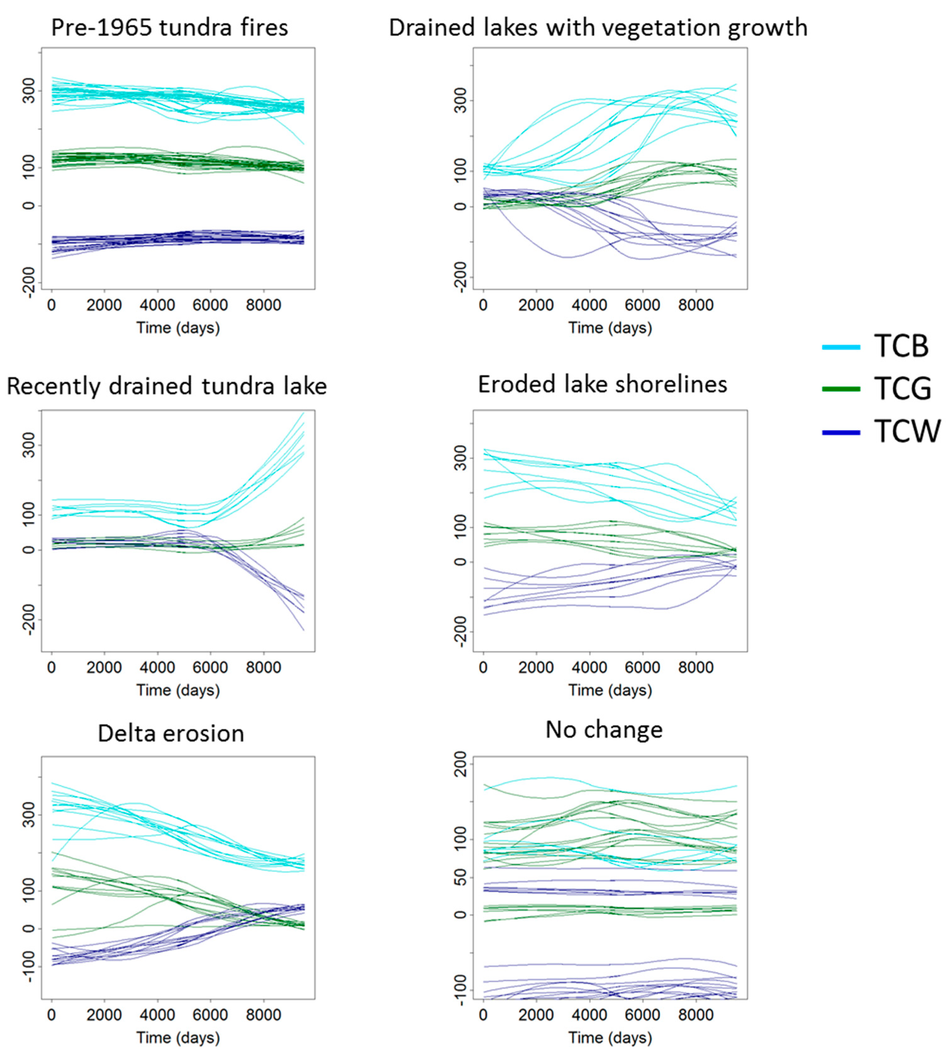
Region 2 loess-smoothed Tasseled Cap disturbance trajectories were plotted as a function of time for individual polygons by disturbance type, revealing high consistency among profiles for certain disturbance types and lower consistency for others. In some cases, it appears that low consistency is caused by differences in the timing of disturbance events, especially for abrupt inter-annual disturbances such as fire. Other changes exhibited relatively consistent trajectories, particularly subtle and progressive processes such as regeneration or greening. Consistency relates partly to the nature of the disturbance itself (e.g., greening is driven by climate factors), but perhaps more so to the number and location of samples that were collected. An insufficient number of samples existed for certain disturbance types to assess their level of consistency altogether.

Figure 4 shows examples of relatively consistent disturbance profiles in the left column and less consistent profiles on the right. Relatively consistent profiles in the database include pre-1965 tundra fires that exhibit a slight decrease in both Tasseled Cap Brightness and Greenness and a slight increase in Wetness. These trajectories reflect late regeneration and early succession due to increasing leaf area index and biomass that is sometimes accompanied by a species shift from broadleaf to needleleaf. Trajectories for recently drained tundra lakes appear to be temporally aligned with the event occurring sometime mid-time-series. This temporal alignment reflects the fact that lakes in the training database likely drained around the same time; however, the shape and magnitude of trajectories are also similar. Following drainage, Brightness increases and Wetness decreases rapidly due to replacement of water with brighter sediment, with the shape of these disturbance trajectories alluding to the potential of second-order polynomial fits to characterize their non-linear nature. Erosion within the Mackenzie Delta is a more progressive disturbance that is opposite as sediment and vegetation are replaced by water.

Examples of less consistent disturbance trajectories include drained lakes with vegetation growth. It should be noted that this is a similar disturbance to recently drained tundra lakes, with the timing of the drainage event being more variable having occurred earlier in (or even prior to) the time-series, thereby allowing vegetation to colonize drained areas and increase Greenness. Eroded lake shoreline disturbance is similar to delta erosion in direction and magnitude of change, but is less similar and less consistent with respect to profile shape. Reasons for this are unknown, but it may relate to a higher percentage of mixed pixels in the sample compared to delta erosion, to variability in the rate of vegetation establishment over bare surfaces among lake slumps or perhaps to different succession due to species differences between the delta and lakeshores. The No-change profiles are also consistent with respect to change magnitude, with relatively flat trajectories through time in all three indices. However, the initial state is the same as the final state with samples representing stable bright targets such as roads, quarries and developments as well as dark targets such as water.

Figure 4. Examples of changes with relatively consistent Tasseled Cap temporal profiles (left column) and inconsistent profiles due to temporal misalignment or the nature of change itself (right column).

Figure 4. Examples of changes with relatively consistent Tasseled Cap temporal profiles (left column) and inconsistent profiles due to temporal misalignment or the nature of change itself (right column).

Table 3. Overall classification accuracies of profile matching by Region.

Profile Matching	Region 2	Region 1	Region 3
Maximum cross-correlation	0.53	0.04	0.21
Minimum Euclidean distance	0.68	0.27	0.37
Minimum Frechet distance	0.69	0.21	0.35

Table 3. Overall classification accuracies of profile matching by Region.

Profile Matching	Region 2	Region 1	Region 3
Maximum cross-correlation	0.53	0.04	0.21
Minimum Euclidean distance	0.68	0.27	0.37
Minimum Frechet distance	0.69	0.21	0.35

4.2. Method Comparison

4.2.1. Temporal-Spectral Profile Matching

Overall classification accuracies for profile matching on all 21 classes based on distance and shape similarity are shown in Table 3. Performance of all three methods was poor even when assessed on a pixel basis over Region 2 that was used to develop the training database. Overall accuracy was considerably lower when profile matching was extended to Regions 1 and 3. Distance metrics performed better than cross-correlation shape matching and despite the fact that neither distance metric accounts for lag, both performed slightly better than the cross-correlation when extended to Regions 1 and 3.

4.2.2. Classification of Trend Coefficients

Overall accuracies for boosted See 5 decision tree classification of regression coefficients are shown in Table 4. For all four regression types, accuracy assessed against training data in Region 2 approached 100% while errors were always less than 10% on individual boosting trails for all regression methods. These results suggest a high level of consistency in the reference data and perhaps over-fitting of models to the training data.

Table 4. Overall classification accuracies of See5 decision tree classification of regression coefficient by Region.

Regression	Region 2	Region 1	Region 3
Linear least-squares	1.00	0.64	0.77
Linear robust (Theil-Sen)	1.00	0.68	0.78
Secord-order polynomial	1.00	0.53	0.66
Third-order polynomial	1.00	0.49	0.64

Table 4. Overall classification accuracies of See5 decision tree classification of regression coefficient by Region.

Regression	Region 2	Region 1	Region 3
Linear least-squares	1.00	0.64	0.77
Linear robust (Theil-Sen)	1.00	0.68	0.78
Secord-order polynomial	1.00	0.53	0.66
Third-order polynomial	1.00	0.49	0.64

Classification accuracies decreased by approximately 20% to 50% when models were extended to Regions 1 and 3, with Region 1 having 10%–15% lower accuracies compared to Region 3. Least-squares and robust Thiel-Sen linear regression outperformed higher-order polynomials, which performed progressively worse from second to third order. This suggests that the non-linear shape of disturbance trajectories may be either too inconsistent within disturbance types or too similar among disturbance types for accurate prediction, or both. This supports the poor results obtained for cross-correlation profile matching that is also based on shape similarity calculated directly between profiles, rather than by use of coefficients describing shape. While coefficients from Thiel-Sen linear regression predict disturbance classes best, least-squares regression that is more sensitive to outliers performs only slightly worse. Fraser et al. [5] noted that visual interpretation of composited TC linear slope images alone was highly effective for discriminating major types of landscape change in the study region.

Table 5 shows average Thiel-Sen coefficients by disturbance type sorted by process. Negative coefficients are highlighted in grey to facilitate visualization. Similarity in the direction and magnitude of change can be seen among several disturbance classes that result from a common underlying process. For example, vegetation succession consistently exhibits a small decrease in Brightness and Greenness and an increase in Wetness, while the initial Tasseled Cap index values indicated by offsets are similar regardless of whether the disturbance class is forest or tundra fire. Regression coefficients of succession processes are similar in direction to those of erosion; however, their magnitude differs especially for slope coefficients that tend to be higher for erosion, suggesting a more pronounced change. Vegetation removal is also consistent with respect to direction and slightly less in magnitude. All three disturbance classes that share this common process exhibit increasing Brightness accompanied by decreasing Greenness and Wetness, with early slump stabilization being a more subtle change as indicated by slightly lower slope magnitude. This consistent Tasseled Cap trajectory of disturbances provides the basis for the Disturbance Index transform for forests [26].

Table 5. Average robust Thiel-Sen regression coefficients by disturbance class sorted by change process. Negative coefficients are shaded to facilitate visualizing similarities between change classes within and between processes.

Change Class	Process	TCB Slope × 10,000	TCB Offset	TCG Slope × 10,000	TCG Offset	TCW Slope × 10,000	TCW Offset
NWT Dated fire surveys	regeneration	17.2	265.9	27.2	75.8	−8.3	−105.6
Older portion of slump	regeneration	34.5	242.9	−7.0	80.7	−38.8	−56.8
Late regeneration	regeneration	13.7	302.9	109.8	43.1	45.6	−121.9
Drained lakes with vegetation growth	emergent vegetation—colonization	220.2	106.3	115.3	−3.6	−135.7	41.7
Conversion of stream bed to vegetation	emergent vegetation—colonization	−43.2	359.9	144.6	12.0	104.5	−178.8
Greening tundra	tundra greening (shrubification)	−1.1	330.2	41.4	99.1	32.1	−142.6
Pre−1965 forest fires	succession	−40.0	275.5	−12.6	105.9	26.0	−79.3
Pre−1965 tundra fires	succession	−39.5	301.9	−19.0	125.1	14.6	−100.0
Development	vegetation removal	87.9	273.5	−86.1	107.6	−77.9	−83.9
Conversion of vegetation to exposed stream bed	vegetation removal	120.9	277.8	−83.4	93.3	−140.2	−59.4
Eroded coastal shorelines	erosion	−155.8	290.2	−40.1	45.6	134.6	−115.1
Eroded lake shorelines	erosion	−119.8	276.9	−48.3	86.4	81.3	−93.1
Active slump	erosion	−66.7	299.4	−48.5	104.3	40.3	−97.3
Active and wet portion of slump	erosion	−124.8	362.5	−91.9	137.8	76.4	−139.8
Conversion of sandbar to stream	erosion	−220.3	357.3	−161.0	153.3	157.0	−105.7
Delta erosion.	erosion	−194.6	350.9	−133.6	137.2	155.2	−87.7
New stream and river sandbars	deposition/drainage	140.7	168.8	−7.6	5.7	−154.0	32.3
Recently drained tundra lake	deposition/drainage	158.6	84.1	5.6	14.8	−106.4	43.4
Delta deposition	deposition/drainage	121.3	183.1	54.7	−2.8	−131.8	25.5
No Change Areas	no change	−1.9	220.3	9.5	59.5	6.8	−57.2
Developed	no change	20.4	301.4	15.3	64.7	6.2	−134.3

Table 5. Average robust Thiel-Sen regression coefficients by disturbance class sorted by change process. Negative coefficients are shaded to facilitate visualizing similarities between change classes within and between processes.

Change Class	Process	TCB Slope × 10,000	TCB Offset	TCG Slope × 10,000	TCG Offset	TCW Slope × 10,000	TCW Offset
NWT Dated fire surveys	regeneration	17.2	265.9	27.2	75.8	−8.3	−105.6
Older portion of slump	regeneration	34.5	242.9	−7.0	80.7	−38.8	−56.8
Late regeneration	regeneration	13.7	302.9	109.8	43.1	45.6	−121.9
Drained lakes with vegetation growth	emergent vegetation—colonization	220.2	106.3	115.3	−3.6	−135.7	41.7
Conversion of stream bed to vegetation	emergent vegetation—colonization	−43.2	359.9	144.6	12.0	104.5	−178.8
Greening tundra	tundra greening (shrubification)	−1.1	330.2	41.4	99.1	32.1	−142.6
Pre−1965 forest fires	succession	−40.0	275.5	−12.6	105.9	26.0	−79.3
Pre−1965 tundra fires	succession	−39.5	301.9	−19.0	125.1	14.6	−100.0
Development	vegetation removal	87.9	273.5	−86.1	107.6	−77.9	−83.9
Conversion of vegetation to exposed stream bed	vegetation removal	120.9	277.8	−83.4	93.3	−140.2	−59.4
Eroded coastal shorelines	erosion	−155.8	290.2	−40.1	45.6	134.6	−115.1
Eroded lake shorelines	erosion	−119.8	276.9	−48.3	86.4	81.3	−93.1
Active slump	erosion	−66.7	299.4	−48.5	104.3	40.3	−97.3
Active and wet portion of slump	erosion	−124.8	362.5	−91.9	137.8	76.4	−139.8
Conversion of sandbar to stream	erosion	−220.3	357.3	−161.0	153.3	157.0	−105.7
Delta erosion.	erosion	−194.6	350.9	−133.6	137.2	155.2	−87.7
New stream and river sandbars	deposition/drainage	140.7	168.8	−7.6	5.7	−154.0	32.3
Recently drained tundra lake	deposition/drainage	158.6	84.1	5.6	14.8	−106.4	43.4
Delta deposition	deposition/drainage	121.3	183.1	54.7	−2.8	−131.8	25.5
No Change Areas	no change	−1.9	220.3	9.5	59.5	6.8	−57.2
Developed	no change	20.4	301.4	15.3	64.7	6.2	−134.3

4.3. Final Classification

The final disturbance classification was obtained by training a boosted See 5 decision tree using Thiel-Sen linear trend coefficients of TCB, TCG and TCW from all 62,509 reference pixels from the three Regions. Accuracy was estimated using 100 bootstrap cross-validation iterations against pixels contained in independent held-out polygons as described in the methods section. This assessment should provide a more realistic accuracy of the final map compared to the approach used in the method evaluation section because it does not depend on spatial extrapolation across a latitudinal gradient. Rather, evaluation is based on interpolation due to the fact that most test polygons will have training data located in all directions.

Table 6. Overall classification accuracy obtained using 100 cross-validation iterations and different percentages of training and test data.

Training	Test	Overall Accuracy
50%	50%	81.6%
75%	25%	82.8%

Table 6. Overall classification accuracy obtained using 100 cross-validation iterations and different percentages of training and test data.

Training	Test	Overall Accuracy
50%	50%	81.6%
75%	25%	82.8%

Overall classification accuracies shown in Table 6 suggest a minimal dependence on the percentage split into training/test data, with overall accuracies in the range of 82% ± < 1%. Attribute usage refers to variable importance in the decision tree model and is reported in descending order for each iteration. Variable rank was summed across 100 iterations to assess overall variable importance (Table 7). TCB slope has the lowest sum of ranks and is therefore the most important variable for change prediction for disturbances in this region. Greenness offset and slope are next followed by brightness offset and finally wetness offset and slope. Regression offsets are shown to be important predictors of disturbance type. Offsets represent the initial surface condition and therefore help specify the nature of change by placing it in context. For example, both regeneration and tundra greening may be changing at a similar rate as measured by Greenness slope, but their initial condition measured by Greenness offset specifies either tundra or forest and dictates the disturbance type.

Table 7. Sum of ranks of variable importance over 100 decision tree model iterations.

Coefficient	Sum of Ranks
TCB_slope	134
TCG_offset	236
TCG_slope	333
TCB_offset	401
TCW_offset	433
TCW_slope	563
1–6 in order of variable importance

Table 7. Sum of ranks of variable importance over 100 decision tree model iterations.

Coefficient	Sum of Ranks
TCB_slope	134
TCG_offset	236
TCG_slope	333
TCB_offset	401
TCW_offset	433
TCW_slope	563
1–6 in order of variable importance

The final assessment is for the 75%/25% training/test data split with a confusion matrix (not shown) generated from the sum of matrices from the 100 cross-validation iterations. Confusion exists between fire classes, particularly among fires that occurred before and during the Landsat time-series. Confusion also occurs between fire and other regeneration classes in slumps and landslides along rivers. Trajectories are similar in both cases, going from dark char or dark soil towards green emergent vegetation. Fire is also misclassified with vegetation removal depending on timing, as confusion with regeneration likely occurs more for fires that happened early in the time-series, and with vegetation removal for fires that occurred later. Finally, fire may be confused with tundra greening or no change depending on the timing and magnitude of each disturbance type. Fires during the early to midpoint of the Landsat time-series may appear to have remained unchanged when fitting a linear trend if the pre-fire condition and final regeneration condition are similar. Fires occurring during the latter part of the time series will only be represented by a limited number of post-disturbance dates and therefore remain undetected using linear regression analysis.

Other confusion exists for classes that share a common underlying process but occur in different contexts. For example, vegetation removal is a process that is common to both Conversion of vegetation to exposed stream bed and Development, only each takes place in its own context with the former occurring near streams and the latter near human developments. A confusion matrix showing the classification accuracy by change process is shown in Table 8.

At the level of eight change processes compared to 21 change classes, overall accuracy increases from 82.8% to 87.3% and Kappa from 73.4% to 79.7%. Errors of omission (1—producer’s accuracy) and commission (1—user’s accuracy) are well balanced, which suggests that the area undergoing different change processes should be well estimated from this map. Some confusion still exists among similar change processes, for example regeneration and succession. Tundra greening is also confused with regeneration and no change depending on the magnitude of greening and the age/timing of the regeneration. Fraser et al. [5] demonstrate that this confusion can be reduced by visually incorporating contextual information related to the shape and size of change patches, and their geographic setting.

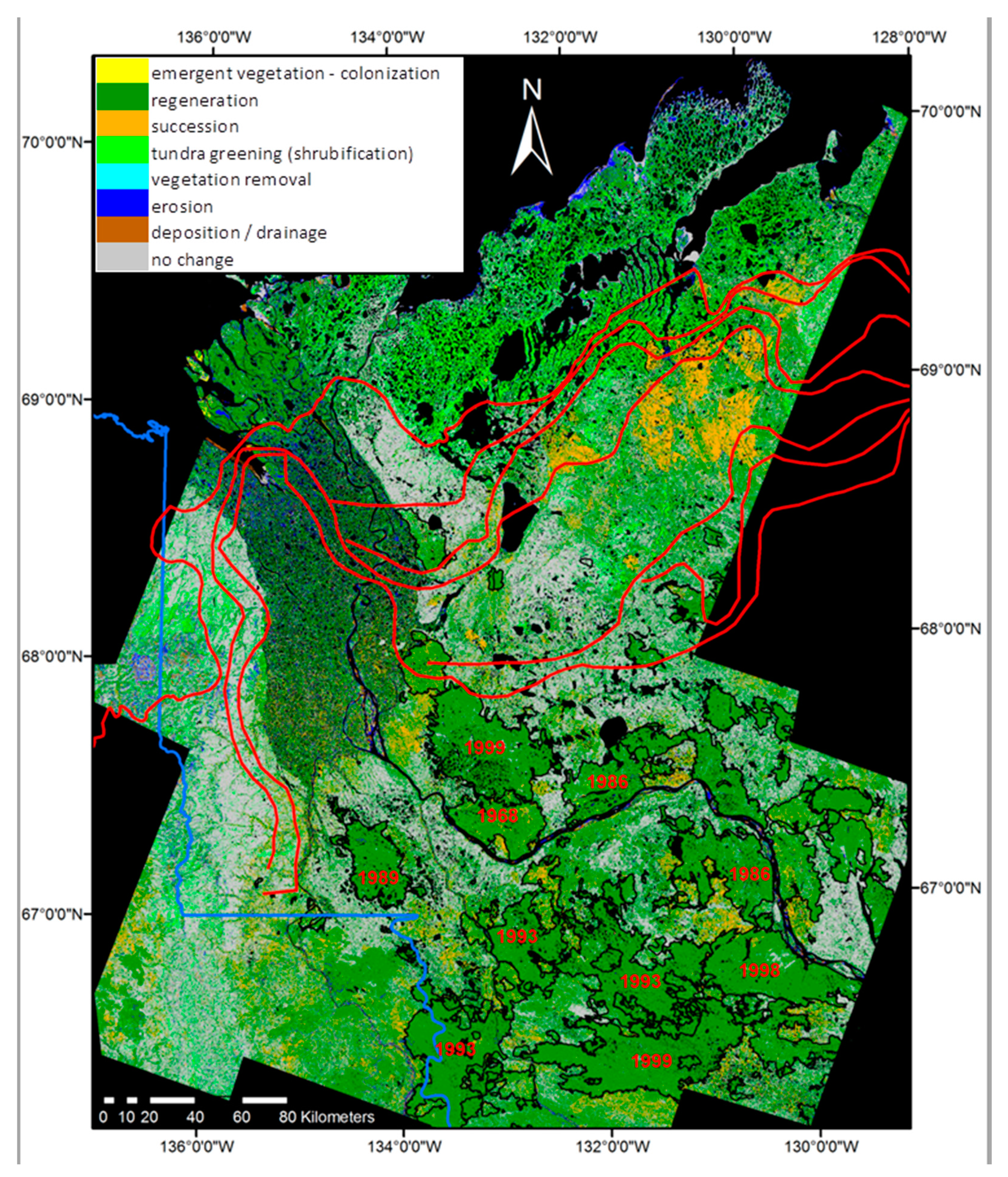
The resulting change process map is shown in Figure 5. Fires appear to be well classified as regeneration when assessed against NWT dated fire polygons. A large area of regeneration also appears at the northern tip of the Mackenzie Delta region that was impacted by a storm surge in 1999. According to [27], 90% of alder shrubs sampled died within five years following the event and soils contained high levels of chloride a decade later, inhibiting vegetation reestablishment. The process labelled “regeneration” largely refers to vegetation removal from fire and assumes subsequent regeneration, though regeneration rates can vary according to fire intensity and location [28]. Both fire and the storm surge appear similar because both maintain dead standing vegetation for a period of time after disturbance as either standing boles in the case of fire or erect dead shrubs following the storm surge. Widespread reestablishment of graminoid and erect shrub began after 2005 and by 2011 roughly two-thirds of the area had exhibited measurable recovery [29].

Tundra greening has occurred extensively above the northernmost treeline isoline and especially on the southern half of the Tuktoyaktuk Peninsula [16]. Along the north shore of the Peninsula and in the northern half of the MacKenzie Delta, there are long stretches of shoreline where erosion has taken place with relatively little deposition, indicating a net loss of land through time [30]. Steeper parts of the Richardson Mountains also show areas of erosion and deposition. Older fires below and within the treeline that pre-date the NWT fire survey beginning in 1965 and are classified as succession. Thaw slumps can be seen east of the Peel River as individual objects classified as erosion. Brooker et al. [31] demonstrated the potential of Landsat Tasseled Cap trends to map and study the evolution of thaw slumps in this region.

Table 8. Confusion matrix from the decision tree classification of eight underlying change processes using robust linear trend coefficients.

		1	2	3	4	5	6	7	8		User’s
1	emergent vegetation—colonization	75,091	6304	3	26	15	593	8022	185		83.2%
2	regeneration	6820	864,658	55,295	9616	3857	6540	823	34,853		88.0%
3	succession	3	26,245	151,045	121	4	626	0	1538		84.1%
4	tundra greening (shrubification)	38	4178	118	40,634	0	66	0	3826		83.2%
5	vegetation removal	42	1865	0	0	14,988	22	12	149		87.8%
6	erosion	625	6374	522	24	53	80,433	30	2102		89.2%
7	deposition/drainage	3021	1049	0	0	211	4	53,689	876		91.2%
8	no change	168	12,421	1080	6532	409	438	72	145,043		87.3%
	Producer’s	87.5%	93.7%	72.6%	71.3%	76.7%	90.7%	85.7%	76.9%
								Overall accuracy:		87.3%
								Kappa:		79.7%

Table 8. Confusion matrix from the decision tree classification of eight underlying change processes using robust linear trend coefficients.

		1	2	3	4	5	6	7	8		User’s
1	emergent vegetation—colonization	75,091	6304	3	26	15	593	8022	185		83.2%
2	regeneration	6820	864,658	55,295	9616	3857	6540	823	34,853		88.0%
3	succession	3	26,245	151,045	121	4	626	0	1538		84.1%
4	tundra greening (shrubification)	38	4178	118	40,634	0	66	0	3826		83.2%
5	vegetation removal	42	1865	0	0	14,988	22	12	149		87.8%
6	erosion	625	6374	522	24	53	80,433	30	2102		89.2%
7	deposition/drainage	3021	1049	0	0	211	4	53,689	876		91.2%
8	no change	168	12,421	1080	6532	409	438	72	145,043		87.3%
	Producer’s	87.5%	93.7%	72.6%	71.3%	76.7%	90.7%	85.7%	76.9%
								Overall accuracy:		87.3%
								Kappa:		79.7%

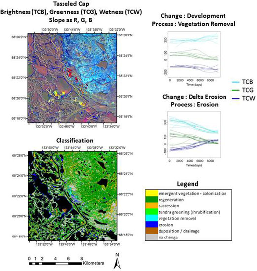
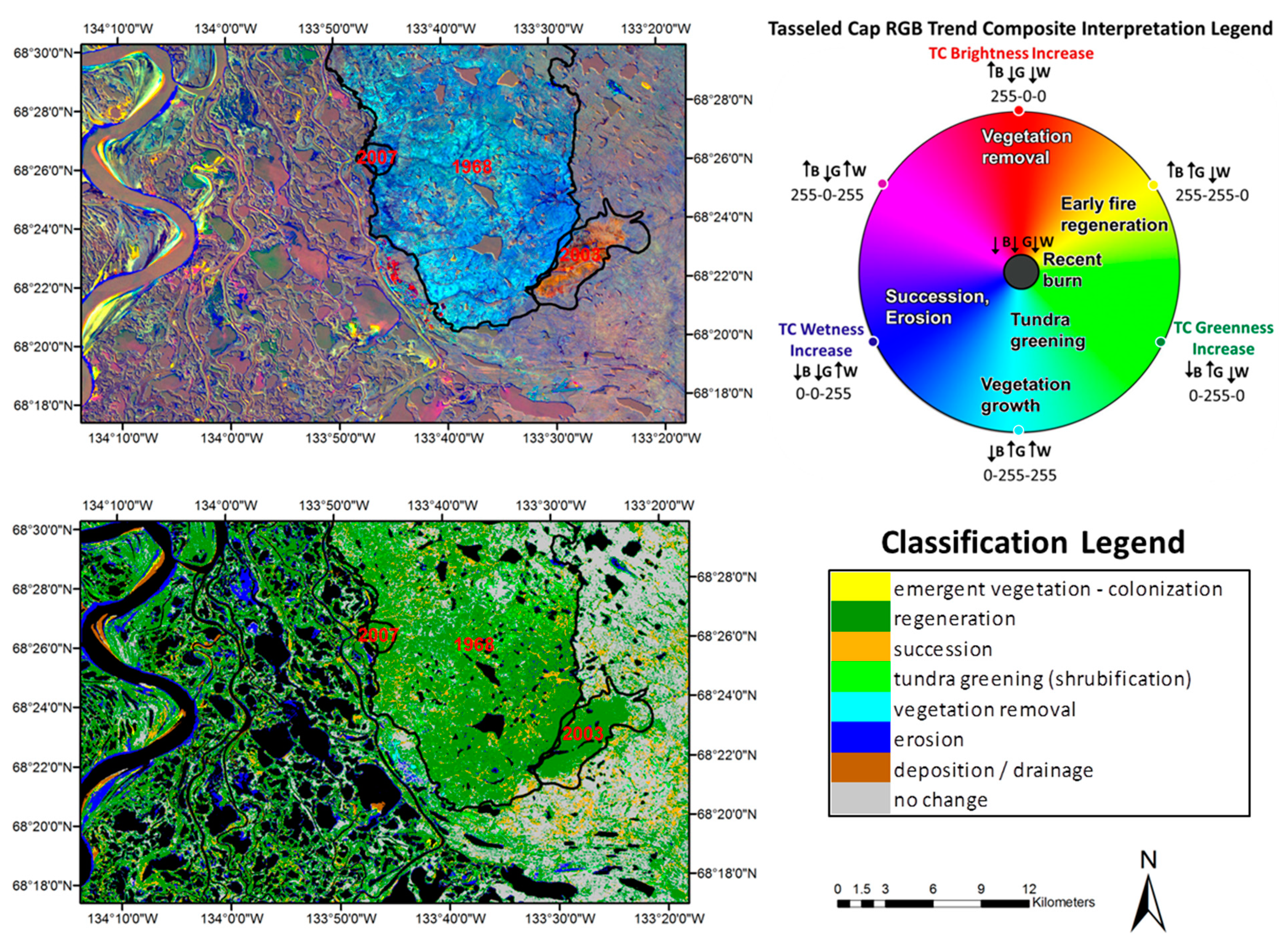
Figure 6 shows an enlargement of the trend composite with interpretation key [5] and classified change process map for the area around Inuvik. A large portion of the northern part of Inuvik is classified as vegetation removal due to recent development. Parts of the delta show vegetation colonization near shore, while elsewhere erosion and deposition occurred. A comparison of both image and map shows the potential utility of each. For a rapid assessment of location and extent of disturbance objects such as thaw slumps, image interpretation and digitizing may be adequate. However, for a survey of the regional extent of different disturbance types, the classified map is perhaps easier and more useful. The accuracy assessment of the map also provides quality assurance of those estimates, while visual interpretation contains error without knowledge of the limitations of derived products. Visual interpretation incorporates context better than automated per-pixel classifiers by relating disturbances to their surroundings. However, regression offsets are also shown to be important predictors of context in decision tree modeling, while trend compositing in Fraser et al. [5] can only visualize regression slopes in the three channels of R, G, B color. An attempt was made to better incorporate context into the decision tree classifier using ancillary layers such as fire, distance to waterbodies, and DEM derivatives, but were found to worsen classification results.

In this study, classification of linear trends outperformed curve matching techniques. Linear trend detection is more suitable for classifying progressive and subtle change, while curve matching should have performed better for detecting sudden change events represented by nonlinear profiles that include inflection points. Because trend detection outperformed profile matching approaches, the methodology may be better suited for mapping progressive change. Although fires were classified well on the basis of their linear vegetation removal or regeneration signal, this was likely because the reference database contained a sufficient range of fires ages that occurred throughout the time-series. Other sudden changes such as human development contained fewer samples and therefore classifying development areas whose timing was not represented in the reference database would be challenging without accounting for temporal alignment. Accuracy may be improved by augmenting the reference database to include more examples of rare disturbances occurring at different times throughout the time-series, or alternatively if real examples do not exist, by generating synthetic samples by offsetting timing information of known examples similar to cross-correlation. An interesting extension of this work would be to explore the use of dynamic time warping approaches for change template matching, which are capable of aligning curves that are out of phase [32,33].

Figure 5. Change map of the Mackenzie Delta region classified to eight change processes. Timoney’s (1992) treeline isolines are in red, the NWT/Yukon border is in blue.

Figure 5. Change map of the Mackenzie Delta region classified to eight change processes. Timoney’s (1992) treeline isolines are in red, the NWT/Yukon border is in blue.

Figure 6. TCB, TCG, TCW displayed as R, G, B and interpretation legend (Fraser et al., this issue [5]) and classified change process map for a region around Inuvik.

Figure 6. TCB, TCG, TCW displayed as R, G, B and interpretation legend (Fraser et al., this issue [5]) and classified change process map for a region around Inuvik.

5. Summary and Conclusions

This study tested methods to classify multi-dimensional spectral trajectories from a Landsat time-series to 21 disturbance classes for cumulative impact assessment in Canada’s Mackenzie Delta region. Curve matching based on shape similarity and distance metrics were tested in addition to decision tree classification using regression coefficients describing profile shape and magnitude. Classification accuracy was found to be poor for the profile matching methods including Euclidean and Frechet distance measures as well as cross-correlation shape similarity, especially when extended to regions beyond the calibration dataset. Decision tree classification generated the best results using robust linear regression coefficients, producing a final map with an overall accuracy of 82.8% that increased to 87.3% when collapsed to eight underlying change processes. Others have employed curve matching to classify change processes [8] in forested regions; however this study presents unique approaches to the problem in an Arctic environment. Other profile matching techniques that can account for temporal misalignment such as dynamic time warping should be considered in future work.

The analysis was limited by a lack of change or disturbance timing information in the reference database that was difficult to obtain, particularly for subtle or ongoing changes such as greening and succession. As a result, each change class was characterized by several profiles that may have been temporally misaligned. In the analysis, we assumed that temporal misalignment could either be accounted for by the profile matching method as is the case for cross-correlation and to a lesser degree Frechet distance, or that the reference data contained a sufficient number of change examples to represent a range of temporal lags, as was demonstrated for fire.

Authors Contribution

Ian Olthof wrote the first draft of the manuscript and was responsible for the research design and leading the data analysis. Robert Fraser supported the interpretation of the results and contributed to writing and editing the manuscript.

References

1. Coppin, P.; Jonckheere, I.; Nackaerts, K.; Muys, B.; Lambin, E. Review ArticleDigital change detection methods in ecosystem monitoring: A review. Int. J. Remote Sens. 2004, 25, 1565–1596. [Google Scholar] [CrossRef]
2. Pouliot, D.; Latifovic, R.; Zabcic, N.; Guindon, L.; Olthof, I. Development and assessment of a 250 m spatial resolution MODIS annual land cover time series (2000–2011) for the forest region of Canada derived from change-based updating. Remote Sens. Environ. 2014, 140, 731–743. [Google Scholar] [CrossRef]
3. Fraser, R.H.; Li, Z.; Cihlar, J. Hotspot and NDVI Differencing Synergy (HANDS): A new technique for burned area mapping over boreal forest. Remote Sens. Environ. 2000, 74, 362–376. [Google Scholar] [CrossRef]
4. Myneni, R.B.; Keeling, C.D.; Tucker, C.J.; Asrar, G.; Nemani, R.R. Increased plant growth in the northern high latitudes from 1981 to 1991. Nature 1997, 386, 698–702. [Google Scholar] [CrossRef]
5. Fraser, R.H.; Olthof, I.; Kokelj, S.V.; Lantz, T.; Lacelle, D.; Brooker, A.; Wolfe, S; Schwartz, S. Detecting landscape changes in high latitude ecosystems using Landsat trend analysis: 1. Visualization. Remote Sens. 2014. [Google Scholar] [CrossRef]
6. Crist, E.P.; Cicone, R.C. A Physically-based transformation of thematic mapper data—The TM tasseled cap. IEEE Trans. Geosci. Remote Sens. 1984, GE-22, 256–263. [Google Scholar] [CrossRef]
7. Roder, A.; Udelhoven, T.; Hill, J.; del Barrio, G.; Tsiourlis, G. Trend analysis of Landsat-Tm and ETM+ imagery to monitor grazing impact in a rangeland ecosystem in Northern Greece. Remote Sens. Environ. 2008, 112, 2863–2875. [Google Scholar] [CrossRef]
8. Kennedy, R.E.; Yang, Z.; Cohen, W.B. Detecting trends in forest disturbance and recovery using yearly Landsat time series: 1. LandTrendr—Temporal segmentation algorithms. Remote Sens. Environ. 2010, 114, 2897–2910. [Google Scholar] [CrossRef]
9. Cohen, W.B.; Yang, Z.; Kennedy, R. Detecting trends in forest disturbance and recovery using yearly Landsat time series: 2. TimeSync—Tools for calibration and validation. Remote Sens. Environ. 2010, 114, 2911–2924. [Google Scholar] [CrossRef]
10. Heginbottom, J.A.; Dubreuil, M.A.; Harker, P.A. Canada—Permafrost. In National Atlas of Canada, 5th ed.; National Atlas Information Service; Natural Resources Canada: Ottawa, ON, Canada, 1995. [Google Scholar]
11. Burn, C.R.; Kokelj, S.V. The environment and permafrost of the Mackenzie Delta area. Permafr. Periglac. Process. 2009, 20, 83–105. [Google Scholar] [CrossRef]
12. Fulton, R.J. Surficial Materials of Canada; Geological Survey of Canada: Ottawa, ON, Canada, 1995. [Google Scholar]
13. Timoney, K.P.; La Roi, G.H.; Zoltai, S.C.; Robinson, A.L. The high subarctic forest-tundra of Northwestern Canada: Position, width, and vegetation gradients in relation to climate. ARCTIC 1992, 45, 1–9. [Google Scholar] [CrossRef]
14. Vincent, L.A.; Wang, X.L.; Milewska, E.J.; Wan, H.; Yang, F.; Swail, V. A second generation of homogenized Canadian monthly surface air temperature for climate trend analysis. J. Geophys. Res. 2012, 117, D18110. [Google Scholar]
15. Serreze, M.C.; Walsh, J.E.; Chapin, F.S., III; Osterkamp, T.; Dyurgerov, M.; Romanovsky, V.; Oechel, W.C.; Morison, J.; Zhang, T.; Barry, R.G. Observational evidence of recent change in the northern high-latitude environment. Clim. Chang. 2000, 46, 159–207. [Google Scholar] [CrossRef]
16. Chander, G.; Markham, B.L.; Helder, D.L. Summary of current radiometric calibration coefficients for Landsat MSS, TM, ETM+, and EO-1 ALI sensors. Remote Sens. Environ. 2009, 113, 893–903. [Google Scholar] [CrossRef]
17. Fraser, R.H.; Lantz, T.C.; Olthof, I.; Kokelj, S.V.; Sims, R.A. Warming-induced shrub expansionand lichen decline in the Western Canadian Arctic. Ecosystems 2014, 17, 1151–1168. [Google Scholar] [CrossRef]
18. Lacelle, D.; Brooker, A.; Fraser, R.H.; Kokelj, S.V. Distribution of thaw slumps and spatio-temporal variations of headwall retreat rates (1990–2010) in the Richardson Mountains—Peel Plateau region, western Arctic Canada. Permafr. Periglac. Process. 2014. submit. [Google Scholar]
19. Olthof, I.; Butson, C.; Fraser, R. Signature extension through space for northern landcover classification: A comparison of radiometric correction methods. Remote Sens. Environ . 2005, 95, 290–302. [Google Scholar] [CrossRef]
20. Alt, H.; Godau, M. Computing the frechet distance between two polygonal curves. Int. J. Comput. Geom. Appl. 1995, 5, 75–91. [Google Scholar] [CrossRef]
21. Song, C.; Woodcock, C.E.; Li, X. The spectral/temporal manifestation of forest succession in optical imagery—The potential of multitemporal imagery. Remote Sens. Environ. 2002, 82, 285–302. [Google Scholar] [CrossRef]
22. Quinlan, J.R. C5: Programs for Machine Learning; Morgan Kaufmann Publishers Inc.: San Francisco, CA, USA, 1993. [Google Scholar]
23. Friedl, M.A.; Brodley, C.E. Decision tree classification of land cover from remotely sensed data. Remote Sens. Environ. 1997, 61, 399–409. [Google Scholar] [CrossRef]
24. Pal, M.; Mather, P.M. An assessment of the effectiveness of decision tree methods for land cover classification. Remote Sens. Environ. 2003, 86, 554–565. [Google Scholar] [CrossRef]
25. Fry, J.; Xian, G.; Jin, S.; Dewitz, J.; Homer, C.; Yang, L.; Barnes, C.; Herold, N.; Wickham, J. Completion of the 2006 national land cover database for the conterminous United States. Photogramm. Eng. Remote Sens. 2011, 77, 858–864. [Google Scholar]
26. Healey, S.P.; Cohen, W.B.; Yang, Z.; Krankina, O.N. Comparison of Tasseled Cap-based Landsat data structures for use in forest disturbance detection. Remote Sens. Environ. 2005, 97, 301–310. [Google Scholar] [CrossRef]
27. Pisaric, M.F.J.; Thienpont, J.R.; Kokelj, S.V.; Nesbitt, H.; Lantz, T.C.; Solomon, S.; Smol, J.P. Impacts of a recent storm surge on an Arctic delta ecosystem examined in the context of the last millennium. Proc. Natl. Acad. Sci. USA 2011, 108, 8960–8965. [Google Scholar] [CrossRef] [PubMed]
28. Johnstone, J.F.; Chapin, F.S., III; Foote, J.; Kemmett, S.; Price, K.; Viereck, L. Decadal observations of tree regeneration following fire in boreal forests. Can. J. For. Res. 2004, 34, 267–273. [Google Scholar] [CrossRef]
29. Lantz, T.; Kokelj, S.V.; Fraser, R.H. Ecological recovery in an arctic delta following widespread saline incursion. Ecol. Appl.  2014, in press. [Google Scholar]
30. Solomon, S.M. Spatial and temporal variability of shoreline change in the Beaufort-Mackenzie region, Northwest Territories, Canada. Geo-Mar. Lett. 2005, 25, 127–137. [Google Scholar] [CrossRef]
31. Brooker, A.; Fraser, R.H.; Olthof, I.; Kokelj, S.V.; Lacelle, D. Mapping the activity and evolution of retrogressive thaw slumps by tasselled cap trend analysis of a Landsat satellite image stack. Permafr. Periglac. Process. 2014. [Google Scholar] [CrossRef]
32. Petitjean, F.; Inglada, J.; Gancarski, P. Satellite image time series analysis under time warping. IEEE Trans. Geosci. Remote Sens. 2012, 50, 3081–3095. [Google Scholar] [CrossRef]
33. Gómez, C.; White, J.C.; Wulder, M.A.; Alejandro, P. Historical forest biomass dynamics modelled with Landsat spectral trajectories. ISPRS J. Photogram. Remote Sens. 2014, 93, 14–28. [Google Scholar] [CrossRef] [Green Version]