Monitoring of Oil Exploitation Infrastructure by Combining Unsupervised Pixel-Based Classification of Polarimetric SAR and Object-Based Image Analysis

Abstract

In developing countries, there is a high correlation between the dependence of oil exports and violent conflicts. Furthermore, even in countries which experienced a peaceful development of their oil industry, land use and environmental issues occur. Therefore, independent monitoring of oil field infrastructure may support problem solving. Earth observation data enables fast monitoring of large areas which allows comparing the real amount of land used by the oil exploitation and the companies’ contractual obligations. The target feature of this monitoring is the infrastructure of the oil exploitation, oil well pads—rectangular features of bare land covering an area of approximately 50–60 m × 100 m. This article presents an automated feature extraction procedure based on the combination of a pixel-based unsupervised classification of polarimetric synthetic aperture radar data (PolSAR) and an object-based post-classification. The method is developed and tested using dual-polarimetric TerraSAR-X imagery acquired over the Doba basin in south Chad. The advantages of PolSAR are independence of the cloud coverage (vs. optical imagery) and the possibility of detailed land use classification (vs. single-pol SAR). The PolSAR classification uses the polarimetric Wishart probability density function based on the anisotropy/entropy/alpha decomposition. The object-based post-classification refinement, based on properties of the feature targets such as shape and area, increases the user’s accuracy of the methodology by an order of a magnitude. The final achieved user’s and producer’s accuracy is 59%–71% in each case (area based accuracy assessment). Considering only the numbers of correctly/falsely detected oil well pads, the user’s and producer’s accuracies increase to even 74%–89%. In an iterative training procedure the best suited polarimetric speckle filter and processing parameters of the developed feature extraction procedure are determined. The high transferability of the methodology is proved by an application to a second SAR acquisition.

1. Introduction

The Doba oil fields were the first of their kind in Chad. Exploration started in 1969 with substantial oil resources being confirmed in the region in 1993. Ten years later, production started in the fields of Miandoum, Bolobo and Komé. Nowadays, the Doba basin in the South of Chad comprises eight oil fields: Moundouli, Miandoum, Nya, Maikeri, Bolobo, Komé, Timbre, and Badila (Figure 1). Four hundred and fifty million barrels of oil have been extracted by the ESSO consortium since production began in late 2003. As a landlocked country, Chad depends on neighboring Cameroon for its oil to reach world markets. A 1070 kilometer export pipeline connects the Doba oil fields with the Gulf of Guinea where offshore infrastructure for storage and vessel loading is located [1].

Figure 1. The study site is located in the Doba basin in southern Chad. The map on the right side shows the oil fields (brown squares) of Komé and its neighborhood as well the study area reported in this article (black rectangle).

Figure 1. The study site is located in the Doba basin in southern Chad. The map on the right side shows the oil fields (brown squares) of Komé and its neighborhood as well the study area reported in this article (black rectangle).

It is well known that the dependence on oil exports often correlates with violent conflicts in developing countries [2]. Chad did not experience the bloodshed and grave human rights violations that characterized the development of neighboring Sudan’s oil industry [3]. Nevertheless, it took place against a backdrop of factional power struggles and a North-South divide as well as authoritarian rule and repression [4]. Trying to avoid the mistakes made in other oil rich countries, a World Bank project was set up to ensure that the local population benefits from oil revenue. Since the Chadian government did not comply with the project requirements, the World Bank abandoned the project in 2008 [4].

In order to prevent land use and environmental issues from arising, independent monitoring of oil field infrastructure is necessary. Satellite data can be analyzed to provide factual evidence on the amount of land used by the oil companies as well as the type of usage. This information can then be checked against the companies’ contractual obligations such as the environment Management Plan which was set up for the Chadian oil fields [5]. These obligations include amongst others the restoration of former oil well pads back into agricultural lands.

Apart from huge infrastructure sites such as central processing facilities, oil fields mainly consist of well pads which either produce oil or inject water into the fields. In the Doba basin, more than 700 well pads are said to be in operation according to the ESSO consortium [6]. The well pads are characterized by flattened, unvegetated rectangles that measure approximately 50–60 m × 100 m. As an exemplary case study, this paper focuses on the study site Komé located in the Doba basin in southern Chad.

The purpose of the research is the detection and monitoring of the implemented infrastructure for oil exploitation—the oil well pads. Especially in remote areas or in cases where field assessments are not possible due to security issues, Earth Observation (EO) data can provide within a short time frame reliable and up to date information on the on-ground situation. Furthermore, space-borne sensors enable the monitoring of a wide field of view (tens of km to more than 100 km) at low costs with a regular revisit time (several days).

The methodology presented in this article is based on polarimetric Synthetic Aperture Radar (SAR) data. SAR has several advantages compared to optical sensors. Contrary to the passive optical sensors which use the solar radiation, SAR as an active sensor is independent of day and night. Moreover, due to its longer wavelength of millimeters to decimeters SAR is almost an all-weather technique, while optical sensors use the visible and infrared part of the electromagnetic spectrum being much more influenced by the atmospheric water vapor. Consequently, in most cases, SAR EO imagery of the Area of Interest (AoI) is earlier available than cloud free optical data [7].

Compared to single polarized SAR data, dual- or quad-polarimetric SAR imagery provides much more information about the backscattering mechanism of the ground target. Therefore, polarimetric SAR data (PolSAR) enables more detailed land cover and land use classification [8,9,10,11].

This article presents an automatic feature extraction procedure based on very high spatial resolution dual-polarimetric SAR imagery of TerraSAR-X, enabling the detection and monitoring of the aforementioned oil exploitation infrastructure (oil well pads). The methodology combines a pixel-based classification of the PolSAR data with an object-based post-processing refinement of the classification.

2. Study Site and Data

The study area (ca. 8.5°N/16.7°E) covers an area of 15 km × 11 km within the Komé oil field which is located in the Doba basin in southern Chad, approximately 430 km south of the Chads capital city Ndjamena (Figure 1). The AoI is characterized by rural area with closed to open shrub land as main land cover [12]. The target features (oil well pads) to be extracted can be characterized as vegetation-free, rectangular patches of land of about 50–60 m × 100 m size (Figure 2).

Figure 2. Subset of the study area. TerraSAR-X acquisition (5 September 2010) (left); Reference dataset marking the features of interest (right), i.e., the oil well pads. The reference oil well pads were generated by manual digitalization. TerraSAR-X © 2014 German Aerospace Center (DLR), 2014 Airbus Defence and Space/Infoterra GmbH.

Figure 2. Subset of the study area. TerraSAR-X acquisition (5 September 2010) (left); Reference dataset marking the features of interest (right), i.e., the oil well pads. The reference oil well pads were generated by manual digitalization. TerraSAR-X © 2014 German Aerospace Center (DLR), 2014 Airbus Defence and Space/Infoterra GmbH.

The developed feature extraction procedure is based on very high spatial resolution dual-polarimetric SAR data of TerraSAR-X (High Resolution SpotLight mode; Polarization HH/VV). The methodology is trained using a first SAR image acquired on 5 September 2010 (cf. Section 3 and Section 4.1). To test the transferability of the developed feature extraction procedure (cf. Section 4.2), the methodology was again applied to a second acquisition from 19 October 2010, using the same imaging parameters (cf. Table 1).

Table 1. Details of used SAR data sets.

Sensor	Imaging Mode	Acquisition Date (Day/Month/Year)	Polari-zation	Incidence Angle (°)	Pass Direction	Relative Orbit
TerraSAR-X	High Resolution SpotLight	5 September 2010	HH/VV	59	Ascending	25
TerraSAR-X	High Resolution SpotLight	19 October 2010	HH/VV	59	Ascending	25

Table 1. Details of used SAR data sets.

Sensor	Imaging Mode	Acquisition Date (Day/Month/Year)	Polari-zation	Incidence Angle (°)	Pass Direction	Relative Orbit
TerraSAR-X	High Resolution SpotLight	5 September 2010	HH/VV	59	Ascending	25
TerraSAR-X	High Resolution SpotLight	19 October 2010	HH/VV	59	Ascending	25

3. Method

The developed procedure can be divided into four main parts, starting with (I) the polarimetric speckle filtering, followed by (II) the decomposition of the polarimetric SAR data to derive information of the physical scattering mechanism of the ground targets. The decomposition parameters are then used as input for (III) a pixel-based unsupervised classification followed by (IV) a hereon based object-based feature extraction. The former (III) aims to extract the land cover/land use class which contains the feature we are interested in—bare land free of vegetation (the oil well pads). The latter (IV) focuses on the refinement of the classification result using Object-Based Image Analysis (OBIA) techniques based on criteria such as shape and minimum area (Figure 3).

3.1. Polarimetric SAR Data Processing

Data from PolSAR systems enable an improved classification of the land cover compared to imagery from single polarized SAR sensors [9,10]. Objects on the ground characterized by different structures and geometries show different backscatter of the SAR wave at different SAR polarizations. Based on physical assumptions, polarimetric decomposition procedures aim to separate these different backscatter types [8,11].

3.1.1. Polarimetric Speckle Filtering

The speckle effect strongly complicates the visual interpretation and the classification of SAR images. The speckle in SAR images is caused by the interference of the coherent reflected SAR waves of many individual scatterers within a resolution cell (distributed targets). Therefore, the first step of the procedure presented in this article is polarimetric speckle filtering to reduce the influence of this effect.

As the developed procedure is based on single acquisitions, only speckle filters working in the spatial domain can be applied (no multi-temporal speckle filters).

We tested three types of polarimetric speckle filters with different parameters (cf. Section 3.1.4)—(I) the mean (box car) filter, (II) the refined Lee filter [13,14] and the (III) Intensity-Driven Adaptive-Neighborhood (IDAN) technique [15,16].

The mean filter assigns the mean of an N × N pixel neighborhood (e.g., for N = 3, there are 8 neighbors) to the center pixel. In contrast to the aforementioned mean filter, the refined Lee filter considers also the structure of the image. This speckle filter is much better suited to preserve edges, which get blurred by the mean filter. The refined Lee filter searches for edges in four directions: horizontal, vertical and the two diagonal directions. The alignment of the edges is determined based on the span image, which is the total scattered power in the case of polarimetric SAR (see Equation (1), valid for the co-dual-polarimetric case HH/VV; with Sinclair-Matrix S, see Equation (3)).

$$Span={\left[S_{HH}\right]}^2+{\left[S_{VV}\right]}^2$$

(1)

Next, the covariance matrix is filtered. The refined Lee filter preserves the correlation between the different polarizations [13,14].

Speckle reduction by the IDAN filter is based on the multiplicative noise model. The basic idea of the IDAN filter is region growing into areas of similar statistical properties [15,16]. This speckle filter is very suited to remove the speckle at large homogenous areas, such as the oil well pads we are interested in.

Figure 3. Procedure of the oil well pad feature extraction (iterations only at training).

Figure 3. Procedure of the oil well pad feature extraction (iterations only at training).

3.1.2. Polarimetric Decomposition

The Jones-Vector is derived from the Maxwell Equation and consists of a field vector of a horizontal E_H and vertical E_V oscillation. Each single oscillation is described by an amplitude γ and a phase value φ (Equation (2)).

$$\overrightarrow{E}=\left[\begin{array}{c}{E}_H\\ E_V\end{array}\right]=\left[\begin{array}{c}{\gamma }_H{e}^{i\phi H}\\ {\gamma }_V{e}^{i\phi V}\end{array}\right]$$

(2)

The Sinclair-Matrix S describes the relation of the transmitted and received wave (Equation (3))

$${\left[\begin{array}{c}{E}_H\\ E_V\end{array}\right]}_{received}=\left[\begin{array}{cc}{S}_{HH}& S_{HV}\\ S_{VH}& S_{VV}\end{array}\right]·{\left[\begin{array}{c}{E}_H\\ E_V\end{array}\right]}_{transmitted}$$

(3)

with S_x,y representing the four combinations of transmitted (index y) and received polarization (index x). If the transmit and receive antennas coincide, S_HV = S_VH = S_X, which reduces S to (Equation (4)):

$$S=\left[\begin{array}{cc}{S}_{HH}& S_X\\ S_X& S_{VV}\end{array}\right]$$

(4)

Enabling also the description of parts of the Sinclair-Matrix elements, the Bourgeaud-Vector is described as follows (Equation (5)):

$${\overrightarrow{S}}_{Bourgeaud}= {\lceil \begin{array}{ccc}{S}_{HH}& \sqrt{2}{S}_X& S_{VV}\end{array}\rceil }^T$$

(5)

The covariance matrix C is defined as the expected value of ${\overrightarrow{S}}_{Bourgeaud}·{{\overrightarrow{S}}^{*T}}_{Bourgeaud}$ (Equation (6)):

$$\langle C_3\rangle = \langle \left[\begin{array}{ccc}{\left|S_{HH}\right|}^2& \sqrt{2}{S}_{HH}{S}_X^{*}& S_{HH}{S}_{VV}^{*}\\ \sqrt{2}{S}_X{S}_{HH}^{*}& 2{\left|S_X\right|}^2& \sqrt{2}{S}_X{S}_{VV}^{*}\\ S_{VV}{S}_{HH}^{*}& \sqrt{2}{S}_{VV}{S}_X^{*}& {\left|S_{VV}\right|}^2\end{array}\right]\rangle$$

(6)

C₃ describes the quad-polarimetric case with the availability of all four combinations of S_x,y. As mentioned in Section 2, our analysis is based on co-polarized dual-polarimetric SAR data (HH and VV). In this case C₃ reduces to C₂ (Equation (7)):

$$\langle C_2\rangle = \langle \left[\begin{array}{cc}{\left|S_{HH}\right|}^2& S_{HH}{S}_{VV}^{*}\\ S_{VV}{S}_{HH}^{*}& {\left|S_{VV}\right|}^2\end{array}\right]\rangle$$

(7)

The anisotropy/entropy/alpha (A/H/α) decomposition proposed by [17] is based on the eigenvalues λ₁, λ₂ and λ₃ of C₃ or C₂. The α angle describes the type of backscattering. Very small α values (close to zero) indicate domination of surface scattering (single bounce scattering) within the resolution cell. High α values represent domination of double bounce scattering, which indicates either urban area or tree trunks. α values in between the aforementioned extremes (i.e., around 45°) show domination of volume scattering, caused by dense vegetation, e.g., multiple scattering inside a volume such as the crown of a tree [18]. α_m represents the mean of α₁ and α₂, with the former describing the backscattering type of the dominant scatterer and the latter the backscattering type of the second dominant one (Equation (8)):

$${\alpha }_m=\frac{1}{{\lambda }_1+{\lambda }_2}·\left[\begin{array}{cc}{\lambda }_1& {\lambda }_2\end{array}\right]·\left[\begin{array}{c}{\alpha }_1\\ {\alpha }_2\end{array}\right]$$

(8)

The second parameter, the entropy H, represents the heterogeneity of the scattering (Equation (9)). H ranges from 0, which indicates a pure target (i.e., a dominant scatterer such as a corner reflector) to 1, representing a random mixture of scattering mechanisms (e.g., forest areas).

$$H=\frac{-1}{{\lambda }_1+{\lambda }_2}·\left[\begin{array}{cc}{\lambda }_1& {\lambda }_2\end{array}\right]·{\log }_2\left(\frac{1}{{\lambda }_1+{\lambda }_2}·\left[\begin{array}{c}{\lambda }_1\\ {\lambda }_2\end{array}\right]\right)$$

(9)

As the interpretation of H values in between the two extremes 0 and 1 is very difficult, a third parameter, the anisotropy A, is used. In practice, A is very important for H > 0.7. In general (i.e., in the full quad-polarimetric case), A enables the investigation of the relationship between the second and third backscattering mechanism (Equation (10)).

$$A_{quad}=\frac{{\lambda }_2-{\lambda }_3}{{\lambda }_2+{\lambda }_3}$$

(10)

However, as we use dual-polarimetric SAR data in our approach, the determination of the third eigenvalue λ₃ is not possible. A reduces in the dual-polarimetric case to (Equation (11)):

$$A_{dual}=\frac{{\lambda }_1-{\lambda }_2}{{\lambda }_1+{\lambda }_2}$$

(11)

For the practical implementation of the developed feature extraction method we used the open source software PolSARpro [19]. This software uses following condition for the calculation of the anisotropy A for the partial polarimetric case (e.g., dual-polarimetric): A is equivalent and equal to the Wave Degree of Polarization (DoP). The DoP ranges from DoP = 0 (representing totally depolarization of the wave) to DoP = 1 (fully polarized waves) [19,20].

3.1.3. Unsupervised Wishart Classification

Next, based on the polarimetric decomposition parameters H, A and α an unsupervised Wishart classification is applied to derive the land cover of the AoI. Two classifications were applied: The first classification is based on H and α only and the second one uses in addition the anisotropy parameter A. The Wishart polarimetric classification procedure executes a Maximum Likelihood (ML) statistical segmentation of a polarimetric data set based on the multivariate complex Wishart probability density function. The initialization of the different clusters uses the result of the H/α segmentation (Figure 4) [21]. Next, a second Wishart classification is applied based on all three components: A/H/α [19]. Thereby, the segmentation shown in Figure 4 is extended to three dimensions, i.e., each zone of the H/α plane is divided into two by using A = 0.5 as cutoff point [20,22]. The Wishart classification procedure executes 10 iterations. The cluster centers initialized by the H/α (or A/H/α) segmentation move during these iterations. Therefore, after several iterations a cluster center may move from one segmentation section to a neighboring section (for instance from class 1 to class 4 (in Figure 4)—These two cluster centers within class 4 (the original class 4 and the one moved from 1 to 4) would then represent two types of double bouncing caused by forest or urban constructions, respectively) [20].

The H/α segmentation plane can be divided into nine segments of which eight are feasible (Figure 4). For instance, very low α and H values are interpreted as bragg surface scattering (“9” in Figure 4) such as bare land (e.g., the oil well pads) or water surfaces. Increasing H, leads to random surface scattering (“6”), i.e., rougher surfaces. Increasing the α value, leads to vegetated areas (“5”) and for very high H values even in random scattering such as forest canopy (“2”). Very high H and α represent complex scattering, e.g., multiple scattering in the crown of a tree (“1”). When again decrease the H value at still high value for α (“4”), we reach double bounce reflections caused by either urban constructions or double bounce between ground and tree trunks (for larger wavelength such as L- and P-band passing through the canopy [10]), and at very low H values dihedral reflections caused by metallic objects such as corner reflectors (“7”). (“8”) represents isolated dipole scatterer, e.g., scattering from vegetation with strongly correlated orientation of anisotropic scattering elements.

Figure 4. H/α segmentation plane (modified after [20]). The numbers represent different types of backscattering as described in the text. The oil well pads—characterized as areas free of vegetation—are located within segment “9”. The grey colored area including “3” is not feasible.

Figure 4. H/α segmentation plane (modified after [20]). The numbers represent different types of backscattering as described in the text. The oil well pads—characterized as areas free of vegetation—are located within segment “9”. The grey colored area including “3” is not feasible.

The classification result is terrain corrected and geocoded, i.e., transformed from the typical SAR geometry (range/azimuth) into a projected coordinate system. The terrain correction is based on a Digital Elevation Model (DEM) of the Shuttle Radar Topography Mission (SRTM) [23].

3.1.4. Iterative Process to Find the Best Suited Combination for the Pixel-Based Classification

In an iterative process, the best suited speckle filter with the best suited parameters (e.g., pixel window) was derived. In order to do this, an accuracy assessment was executed for each combination of polarimetric speckle filters and additional averaging of the Wishart classification (for both H/α and A/H/α). Manually digitalized polygons of our features of interest (the oil well pads) were used as a reference for the accuracy assessment. As basis for the digitalization we used the intensity SAR image (see Figure 2).

The test included all combinations of an N × N pixel window for the speckle filter and an M × M pixel window for the additional filtering of the unsupervised Wishart classification (described in Section 3.1.3). This additional filtering of the classification result applies a box car filtering.

(a) Mean (box car) speckle filter

First, both the entropy H and the angle α (see Section 3.1.2 ) were calculated based on an N × N pixel window with 3 ≤ N ≤ 19 (box car speckle filter, see Section 3.1.1). For the additional filtering of the Wishart classification, we tested 3 ≤ M ≤ 9.

(b) Refined Lee speckle filter

The refined Lee speckle filter (see Section 3.1.1) was calculated for 7 ≤ N ≤ 11 with an additional filtering of the Wishart classification for 1 ≤ M ≤ 9 (with M = 1 representing no additional filtering of the Wishart classification).

(c) Intensity-Driven Adaptive-Neighborhood filter

For the IDAN filter (see Section 3.1.1) the maximum region growing was set to 50 pixels, while the additional filtering of the Wishart classification was applied for 1 ≤ M ≤ 9 (with M = 1 representing no additional filtering of the Wishart classification).

3.2. Object-Based Post-Classification

To improve the classification results of the pixel-based classification described above, in a second step an object-based post-classification is applied. First, morphological procedures such as shrinking and expanding are used to clean the boundaries of the classified objects (especially the oil well pads) and to close small islands within larger objects. Second, an object-based rule-set using the Cognition Network Language (CNL) is applied to extract the oil well pads using criteria such as minimum area, shape and asymmetry. Third, an additional boundary cleaning is applied based on morphological approaches.

After transforming the PolSAR pixel-based classification result presented in Section 3.2 into a binary format (i.e., class “1” = possible oil well pad; class “0” = all other land cover classes), the object-based post-classification starts with the first morphological step: Shrinking of the oil well pads (class 1) by a certain number of pixels s. The shrinking procedure aims to eliminate small areas characterized by the same SAR backscattering properties as the oil well pads, e.g., small areas free of vegetation. After that, an expanding of the oil well pad (class 1) by a certain number of pixels e is applied to (I) close small islands within larger areas of class 1 and (II) to compensate for the previous shrinking—especially at the boundaries of the oil well pad class. Again, within an iterative process the best suited combination of shrinking and expanding is derived by comparing the resulting features with the reference data (see Section 4.1).

Next, an OBIA rule-set is applied to the binary data preprocessed in the aforementioned step. First, the image is segmented using the multiresolution approach based on the Fractal Net Evolution Approach (FNEA) [24,25]. The target features, i.e., the oil well pads, are characterized by a more or less (I) rectangular shape with (II) a size of approximately 50–60 m × 100 m. Furthermore, as we are working with binary data (class 1 = possible oil well pad; class 0 = all other land cover types), the focus at the multiresolution segmentation is at the shape of the target features and not on the spectral information of the imagery (only 2 classes). To consider the shape of the oil well pads, (I) higher shape values (0.8) than color, and (II) high compactness (0.8) compared to smoothness are chosen. Moreover, to take the large areas of our target class into account, (II) a relatively large scale parameter (80) which is an abstract value to determine the maximum possible change of heterogeneity with no direct correlation to the object size measured in pixel is used [26].

Second, all segments of the binary data are classified to the classes “possible oil well pads” and “No Data” (all other land cover classes) based on the binary values “1” or “0”, respectively. Third, all possible oil well pads objects which are smaller than a minimum area of 4500 m² are excluded from this class. As oil well pads have in general a size of 50–60 m × 100 m (see Section 1), the minimum area results in 5000 m². To be able to detect also slightly smaller oil well pads, we applied a 10% buffer in the feature extraction procedure resulting in the aforementioned minimum area of 4500 m².

Fourth, to differentiate between our targets features (i.e., oil well pads) and features of similar SAR backscattering properties, such as unpaved tracks and roads (land cover bare soil, free of vegetation), an arithmetic feature f is calculated for each segment (Equation (12)). The asymmetry (ranging from 0–1) of an object is defined by comparing the length and width of an object. The rectangular fit (ranging from 0–1) calculation is based on a rectangle with the same area and length to width proportion as the object to be analyzed. The overlapping area of the rectangular is compared with the area of the image object outside the rectangle. The higher the overlapping part between image object and comparison rectangular, the higher is the value of the rectangular fit (with 1 = perfect rectangular).

$$f=\frac{Asymmetry}{Rectangular Fit}$$

(12)

The arithmetic feature f considers the more or less rectangular shape of the oil well pads, i.e., low asymmetry and high rectangular fit values. Contrary to this, linear features such as tracks and roads are characterized by high asymmetry values. Consequently, all segments of the class “possible oil well pads” exceeding a value of f > 0.5 are excluded from the target feature class and assigned to the new class “linear objects” (e.g., roads and tracks). This is achieved by first merging all “possible oil well pads” exceeding a certain f value and second excluding all of these newly generated connected objects exceeding a certain area (assigned to the class roads and tracks).

After the OBIA rule-set application an additional combination of shrinking and expanding procedures is used for boundary cleaning of the oil well pad features. The procedure is as follows: e, s, s, e with e = s = 3 pixels showing the best result. Thereby, the boundaries of the oil well pads are smoothed and the accuracy of the feature extraction is in addition slightly increased (see Section 4.1).

4. Results

4.1. Results of the Training Data Set—Development of the Feature Extraction Procedure—Area Based Accuracy Assessment

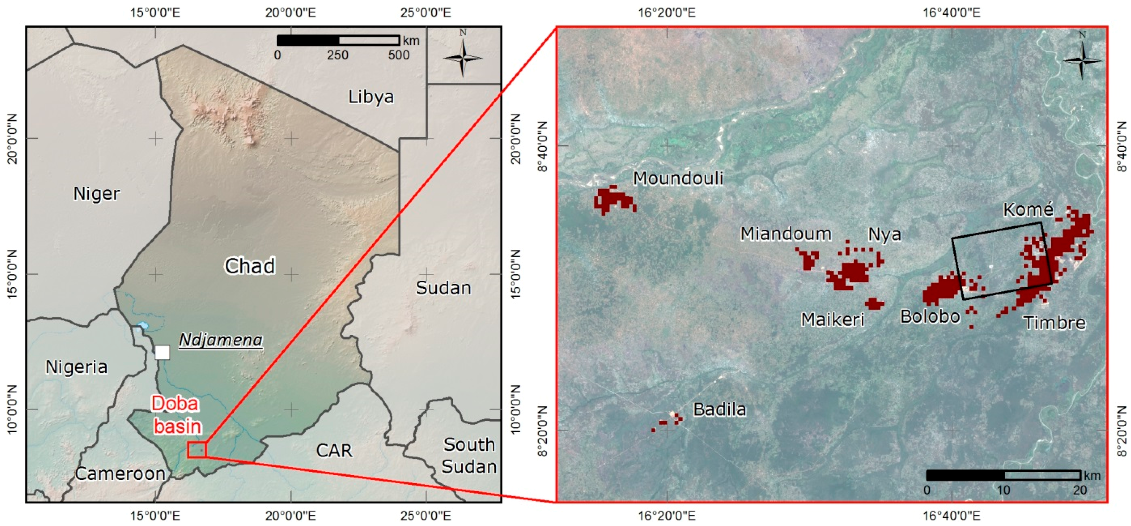
The methodology described in Section 3 was developed using the TerraSAR-X dual-pol High Resolution SpotLight imagery acquired on 5 September 2010. After that the best suited parameters for the oil well pad extraction at this scene were applied to extract the oil well pads at the second acquisition (19 October 2010), enabling a fully automated feature extraction (see Section 4.2).

Figure 5 shows for a subset of the study area the result of the first step—the pixel-based PolSAR Wishart classification (based on H/α). When visually comparing the classification with the reference data (manually digitized polygons), one can recognize that all oil well pads are detected. However, there is also a strong overestimation, as also roads and tracks and other smaller areas free of vegetation (bare land) are classified as the same class as the oil well pads. This is confirmed by the high producer’s accuracy (=high detection rate) of 82.25% or 69.56% for H/α or A/H/α, respectively. The strong overestimation is reflected by the relatively low user’s accuracy of 6.29% or 7.02% for H/α or A/H/α, respectively. The mentioned values for the producer’s and user’s accuracies are valid for the best suited parameters (IDAN 50, M = 9; described in detail below).

Figure 5. Subset of the study area. Left: Original TerraSAR-X acquisition (5 September 2010). Right: Best result of the pixel-based Wishart classification. This first classification step is based on H/α (with M = 9) using the IDAN filter (with 50 pixel max. region growing). Visual comparison with the reference data shows a high detection rate of the oil well pads, but also a strong overestimation (e.g., roads and tracks and other areas of bare land are classified as the same class (class 1, red) as the oil well pads). Visual comparison with optical imagery enables an assignment of the classes to different types of land cover and backscattering mechanisms (cf. also Section 3.1.3): The classes 2, 8, 6 and 7 represent different kinds of double bouncing (segment 4 in Figure 4) caused by urban construction (2 and 8) or forest (6 and 7), respectively. This doubled assignment of the classes (2 and 8 or 6 and 7, respectively) can be explained by different power of backscattering. The classes 3, 4 and 5 represent areas of rougher surfaces with lower vegetation (segment 6 in Figure 4), vegetated areas (segment 5) and forest (segment 2), respectively. TerraSAR-X © 2014 German Aerospace Center (DLR), 2014 Airbus Defence and Space/Infoterra GmbH.

Figure 5. Subset of the study area. Left: Original TerraSAR-X acquisition (5 September 2010). Right: Best result of the pixel-based Wishart classification. This first classification step is based on H/α (with M = 9) using the IDAN filter (with 50 pixel max. region growing). Visual comparison with the reference data shows a high detection rate of the oil well pads, but also a strong overestimation (e.g., roads and tracks and other areas of bare land are classified as the same class (class 1, red) as the oil well pads). Visual comparison with optical imagery enables an assignment of the classes to different types of land cover and backscattering mechanisms (cf. also Section 3.1.3): The classes 2, 8, 6 and 7 represent different kinds of double bouncing (segment 4 in Figure 4) caused by urban construction (2 and 8) or forest (6 and 7), respectively. This doubled assignment of the classes (2 and 8 or 6 and 7, respectively) can be explained by different power of backscattering. The classes 3, 4 and 5 represent areas of rougher surfaces with lower vegetation (segment 6 in Figure 4), vegetated areas (segment 5) and forest (segment 2), respectively. TerraSAR-X © 2014 German Aerospace Center (DLR), 2014 Airbus Defence and Space/Infoterra GmbH.

The validation or accuracy assessment (of Section 4.1 and Section 4.2) was applied to the entire AoI and is based on the comparison of the area of the oil well pads classified by the described methodology with the area of the reference data. This type of accuracy assessment is much more accurate than an accuracy assessment based on only counting the numbers of correctly and falsely detected oil well pads (cf. Section 4.3).

For all tested combinations of different speckle filters (box car, refined Lee, IDAN) and different values for N and M (cf. Section 3.1.4), there is a relatively high overall accuracy ranging between 69% and 97%. Moreover, the user’s and producer’s accuracies for the class “non oil well pads” (i.e., the remaining land cover classes outside the oil well pads) are very high for all the tested combinations (ranging between 90%–99% or 68%–92%, respectively). This effect can be explained by the domination of the class “non oil well pads” regarding the percentage area of the entire study area. Consequently, to analyze the accuracy of the presented feature extraction method, we focus on the user’s and producer’s accuracy of the class oil well pads.

As described in Section 3.1.4 in an iterative process the best suited combination for the pixel-based PolSAR classification was derived.

The Figure 6 and Figure 7 show the user’s accuracy values for the box car filter (with 3 ≤ N ≤ 19 and 3 ≤ M ≤ 9), the refined Lee filter (with 7 ≤ N ≤ 11 and 1 ≤ M ≤ 9) and the IDAN filter (with a maximum region growing of 50 pixels and 1 ≤ M ≤ 9). With M describing the pixel size of the additional filtering of the Wishart classification.

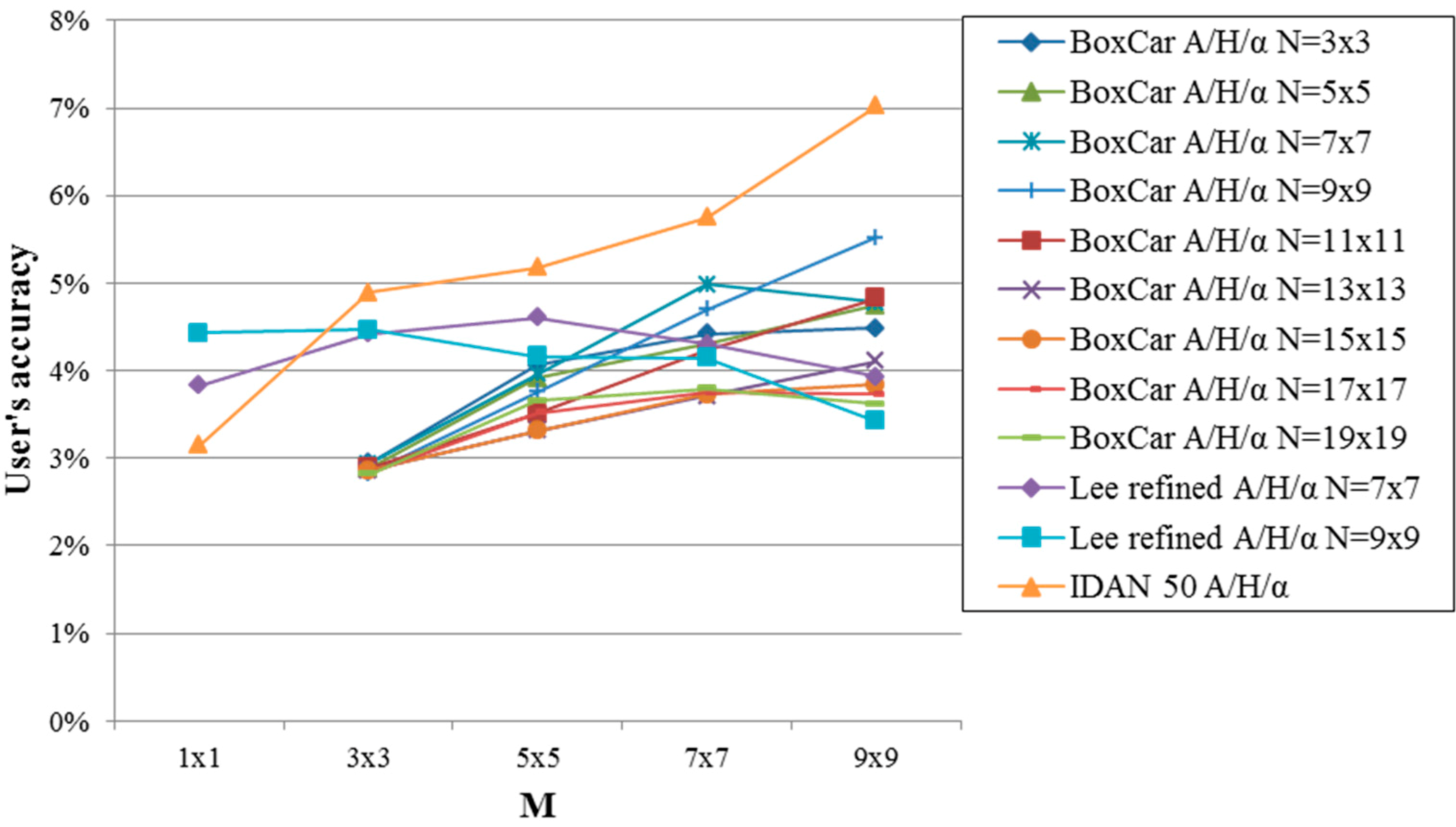
Figure 6. User’s accuracy vs. window size M after the pixel-based PolSAR classification based on H/α (box car, refined Lee and IDAN filter) for the first TerraSAR-X acquisition (5 September 2010).

Figure 6. User’s accuracy vs. window size M after the pixel-based PolSAR classification based on H/α (box car, refined Lee and IDAN filter) for the first TerraSAR-X acquisition (5 September 2010).

Except for N = 3 and N = 19, the box car filter shows an increase of the user’s accuracy with increasing M. All in all, when focusing on the user’s accuracy values at the highest value of M = 9, the user’s accuracy increases with increasing N with the highest value at N = 9. At N > 9, the user’s accuracy decreases again with increasing N. The best result of the box car filter is achieved at N = M = 9.

The refined Lee filter shows an opposed trend. Here, the user’s accuracy decreases with increasing M. The best result for this speckle filter is at N = 7, M = 5.

The best result of all polarimetric speckle filters is achieved by using the IDAN filter (with 50 pixels maximum region growing) and M = 9. This combination achieves the best result of 6.29% for the user’s accuracy (with 82.25% producer’s accuracy) for H/α and 7.02% user’s accuracy (with 69.56% producer’s accuracy) with additionally considering the anisotropy (A/H/α). The achieved Cohen’s Kappa values are 0.10 or 0.11 for H/α or A/H/α, respectively.

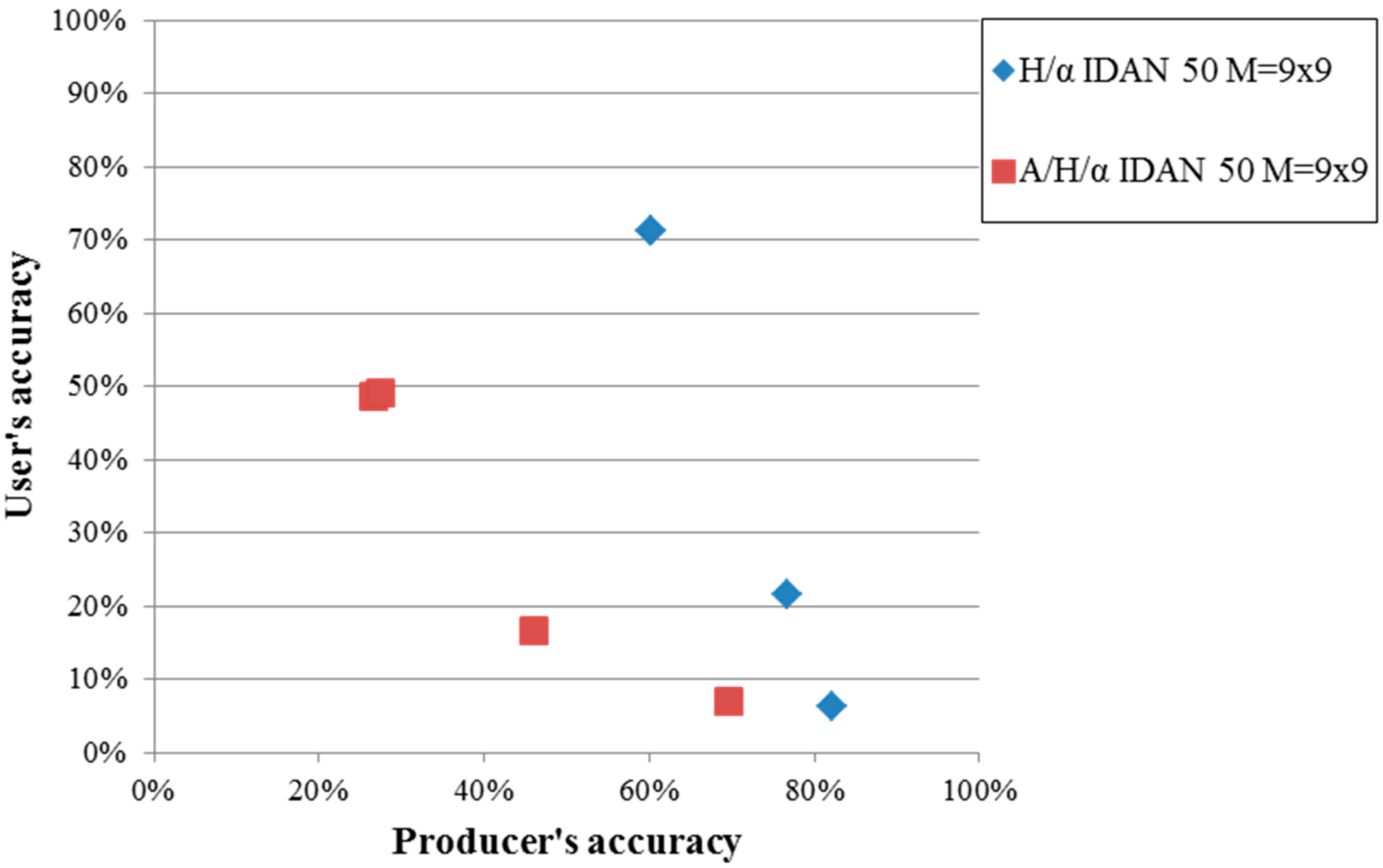
Figure 7. User’s accuracy vs. window size M after the pixel-based PolSAR classification based on A/H/α (box car, refined Lee and IDAN filter) for the first TerraSAR-X acquisition (5 September 2010).

Figure 7. User’s accuracy vs. window size M after the pixel-based PolSAR classification based on A/H/α (box car, refined Lee and IDAN filter) for the first TerraSAR-X acquisition (5 September 2010).

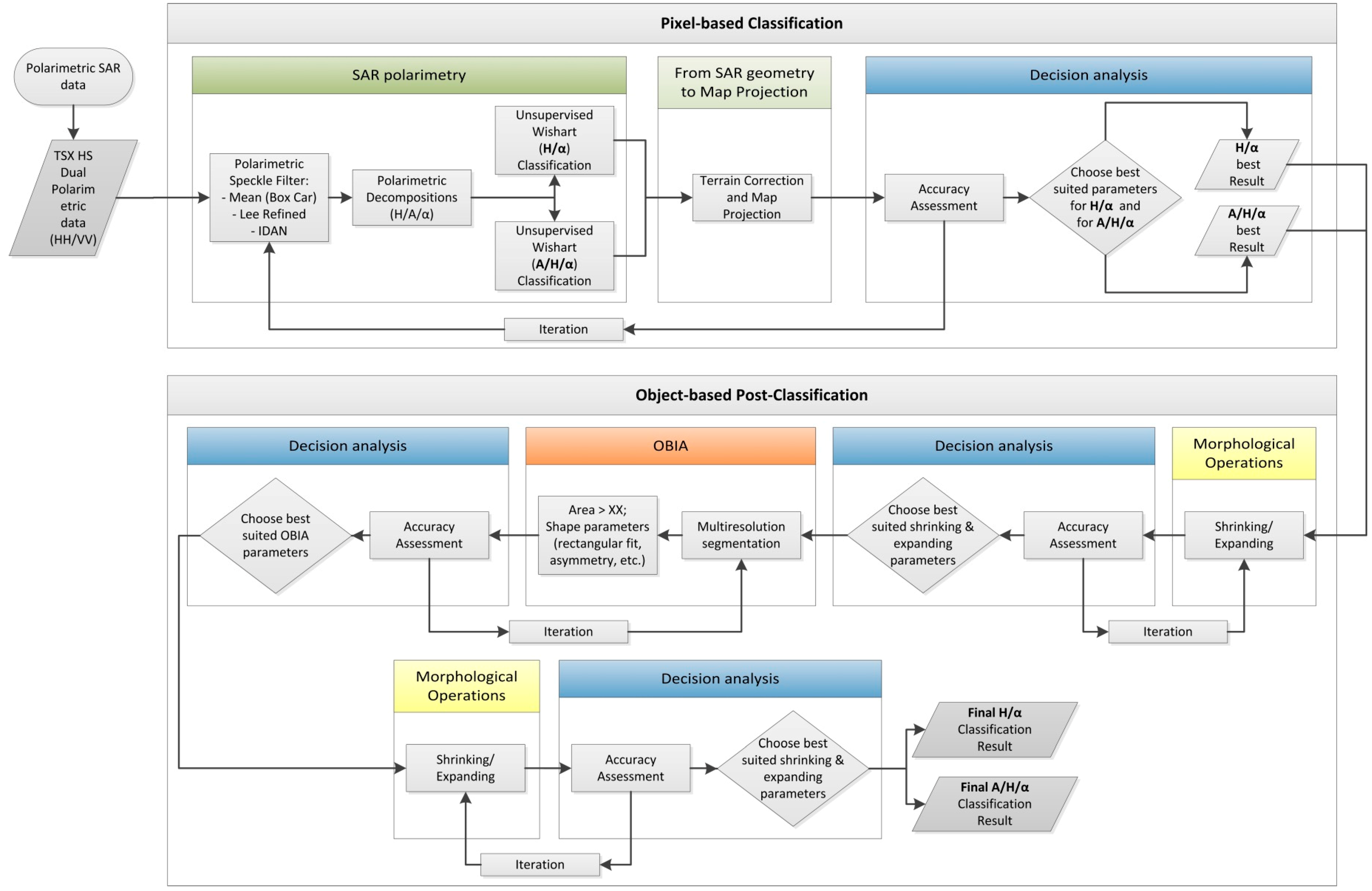
The second part of the developed feature extraction procedure—the object-based post-classification (cf. Section 3.2)—uses the best result of the previous step as input: IDAN filter (with 50 pixels maximum region growing) and M = 9. Figure 8 shows the development of the user’s versus the producer’s accuracy within the object-based refinement for H/α and A/H/α, respectively.

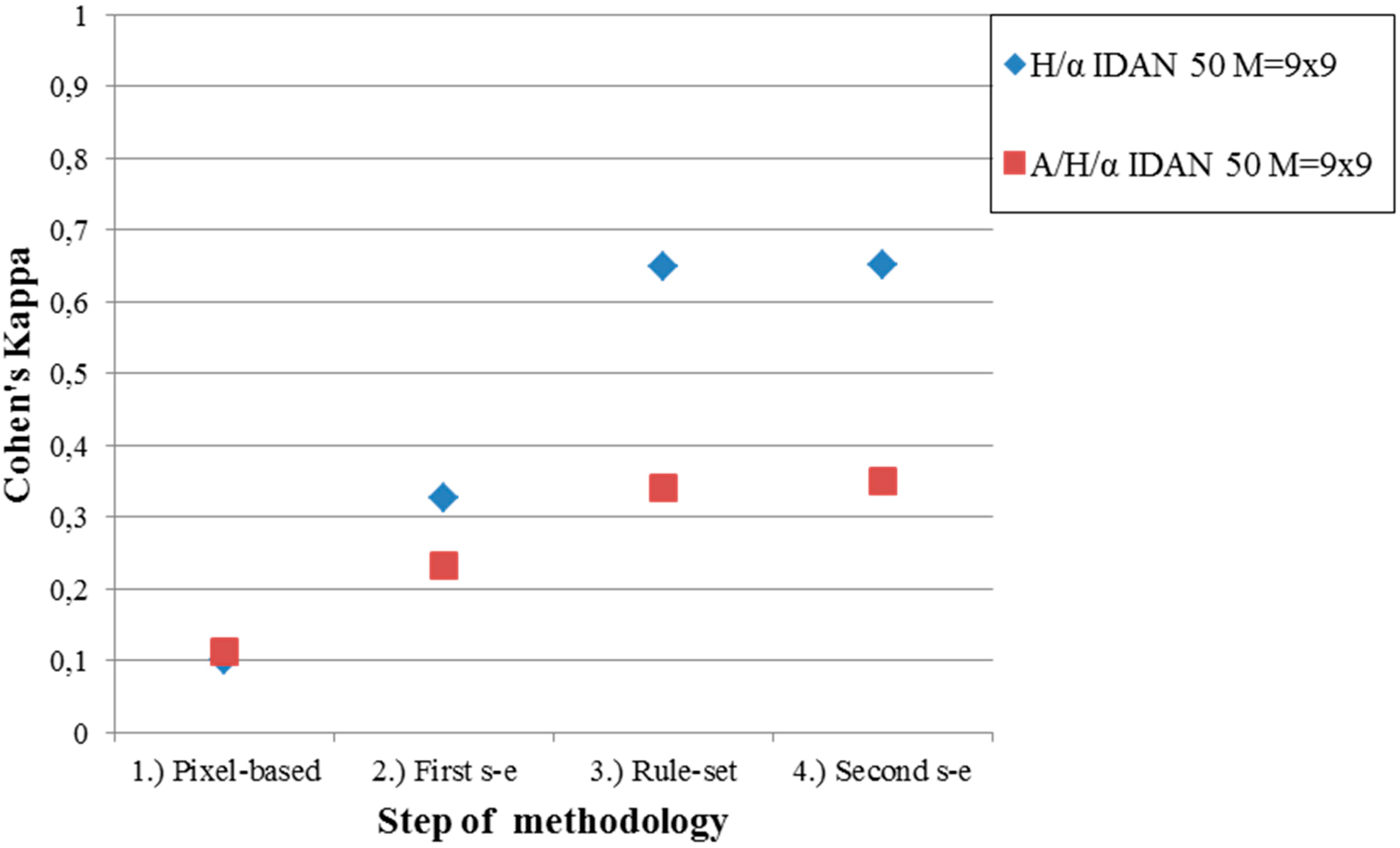
As described in Figure 4, the object-based post-classification starts with shrinking (s) and expanding (e) of the binary data with focus on the possible oil well pads. The best suited results were achieved with s = e = 4 pixels for H/α and s = e = 2 for additionally considering the anisotropy (A/H/α). Thereby, the user’s accuracy of H/α was increased threefold (doubled) from the original 6.29% (7.02% for A/H/α) to 21.54% (16.54%), while the producer’s accuracy of H/α was only slightly reduced from the primary 82.25% (69.56% for A/H/α) to 76.72% (46.13% for A/H/α). The first shrinking and expanding procedure also strongly increased the Cohen’s Kappa value from 0.10 or 0.11 to 0.33 or 0.23 for H/α or A/H/α, respectively (Figure 9).

The second object-based post-classification step includes a rule-set based procedure (cf. Section 3.2) considering the minimum area of the oil well pads, their more or less rectangular shape and the nature of other land cover types characterized by the same backscattering properties (e.g., features free of vegetation with linear shape—high asymmetry—such as roads and tracks). This refinement procedure strongly increased the user’s accuracy of H/α by an order of magnitude (compared to the primary pixel-based classification) to 71.16% (Figure 8). The user’s accuracy of A/H/α increased to 48.72%. The corresponding producer’s accuracy of H/α remains still relatively high with 60.16%. Contrary to this, the producer’s accuracy of A/H/α strongly decreased to 26.63%. This second post-classification step increased the Cohen’s Kappa to 0.65 for H/α (0.34 for A/H/α).

The third step of the object-based refinement is a combination of expanding and shrinking procedures. The best suited results were achieved for a combination of e, s, s, e with e = s = 3 pixels. This last post-classification step has more visual influences, such as cleaning (smoothing) of the boundaries of the extracted oil well pad objects, as the user’s accuracies only slightly increased to 71.28% or 49.19% for H/α or A/H/α, respectively. The corresponding final producer accuracies also slightly increased by this last morphological step to 60.24% or 27.54% for H/α or A/H/α, respectively (Figure 8). The final achieved Cohen’s Kappa value is 0.65 for H/α (0.35 for A/H/α) (Figure 9).

Figure 8. Development of user’s accuracy vs. producer’s accuracy for the OBIA improvements (for the best results of the pixel-based PolSAR classification) based on H/α or A/H/α, respectively (for the first TerraSAR-X acquisition (5 September 2010)). Processing steps from lower right to upper left: (1) pixel-based, (2) first s-e, (3) rule-set, (4) second s-e. Please notice that the third and fourth point are located very close to each other (valid for both, H/α and A/H/α).

Figure 8. Development of user’s accuracy vs. producer’s accuracy for the OBIA improvements (for the best results of the pixel-based PolSAR classification) based on H/α or A/H/α, respectively (for the first TerraSAR-X acquisition (5 September 2010)). Processing steps from lower right to upper left: (1) pixel-based, (2) first s-e, (3) rule-set, (4) second s-e. Please notice that the third and fourth point are located very close to each other (valid for both, H/α and A/H/α).

For sake of completeness, the final values for the overall accuracy and the user’s and producer’s accuracy for the class “non oil well pads” are 99.08%, 99.34% and 99.74%. However, as mentioned in the beginning of this section, these values are not relevant for the validation of this methodology, as the area of the class “non oil well pads” is much larger than the area of the oil well pads. Therefore, the focus is on the user’s and producer’s accuracies of the class “oil well pads”.

The visual comparison of the classification with the reference data (see Figure 10) confirms the high accuracy values of the final result of the oil well pad feature extraction.

In conclusion, Figure 8 clearly demonstrates the surplus value which is achieved by combining a traditional pixel-based classification with an object-based post-classification procedure additionally taking the properties like shape, area and neighboring relations into account.

Figure 9. Development of the Cohen’s Kappa coefficient for the OBIA improvements (for the best results of the pixel-based PolSAR classification) based on H/α or A/H/α, respectively (for the first TerraSAR-X acquisition (5 September 2010)).

Figure 9. Development of the Cohen’s Kappa coefficient for the OBIA improvements (for the best results of the pixel-based PolSAR classification) based on H/α or A/H/α, respectively (for the first TerraSAR-X acquisition (5 September 2010)).

Figure 10. Subset of the study area. Original TerraSAR-X acquisition (5 September 2010) (left). Final result of the feature extraction methodology (right): Combination of the pixel-based PolSAR Wishart classification (based on H/α with M = 9; IDAN filter with 50 pixel max. region growing) with the object-based post-classification. The visual comparison of the classification and the reference data confirms the high accuracy values reported in Figure 8. TerraSAR-X © 2014 German Aerospace Center (DLR), 2014 Airbus Defence and Space/Infoterra GmbH.

Figure 10. Subset of the study area. Original TerraSAR-X acquisition (5 September 2010) (left). Final result of the feature extraction methodology (right): Combination of the pixel-based PolSAR Wishart classification (based on H/α with M = 9; IDAN filter with 50 pixel max. region growing) with the object-based post-classification. The visual comparison of the classification and the reference data confirms the high accuracy values reported in Figure 8. TerraSAR-X © 2014 German Aerospace Center (DLR), 2014 Airbus Defence and Space/Infoterra GmbH.

4.2. Results—Application of the Fully Automated Feature Extraction Methodology to the Second TerraSAR-X Acquisition—Area Based Accuracy Assessment

To investigate the transferability of the PolSAR data based oil well pad feature extraction methodology described in Section 3, the feature extraction procedure was in addition applied to a second High Resolution SpotLight TerraSAR-X acquisition (19 October 2010) recorded ca. 1.5 month later over the same AoI. To enable a fully automated feature extraction and also a direct comparison of the achieved accuracies at the different acquisition dates, the same parameters which worked out to be suited best (see Table 2) during the training procedure based on the first TerraSAR-X acquisition (5 September 2010) (cf. Section 4.1) were used for the processing of the second one (19 October 2010).

Table 2. Best suited parameters for the oil well pad feature extraction derived by the training procedure (based on the TerraSAR-X acquisition 5 September 2010) and applied to the second acquisition (19 October 2010).

Parameter/Processing Step	Value
IDAN speckle filter	50 pixels maximum region growing
M	9
Shrinking, expanding	s = e = 4 for H/α; s = e = 2 for A/H/α
Rule-set	Minimum area, shape, (asymmetry, rectangular fit)
Expanding, shrinking, shrinking, expanding	e = s = 3 for both H/α and A/H/α

Table 2. Best suited parameters for the oil well pad feature extraction derived by the training procedure (based on the TerraSAR-X acquisition 5 September 2010) and applied to the second acquisition (19 October 2010).

Parameter/Processing Step	Value
IDAN speckle filter	50 pixels maximum region growing
M	9
Shrinking, expanding	s = e = 4 for H/α; s = e = 2 for A/H/α
Rule-set	Minimum area, shape, (asymmetry, rectangular fit)
Expanding, shrinking, shrinking, expanding	e = s = 3 for both H/α and A/H/α

Due to changes on the ground in the time period between the two SAR acquisitions (i.e., construction of few new oil well pads by the oil industry), the reference dataset of the first TerraSAR-X acquisition had to be updated. In practice, the topicality of reference dataset was checked based on the second SAR acquisition. New constructed oil well pads were added to the dataset.

Figure 11, the development of the user’s and producer’s accuracies—shows a similar trend for the second TerraSAR-X acquisition (19 October 2010) as the first one (5 September 2010) described in Section 4.1. The PolSAR pixel-based Wishart classification achieved a user’s and producer’s accuracy of 4.83% for H/α (6.00% for A/H/α) and 87.59% (78.62% for A/H/α), respectively. The Cohen’s Kappa was 0.07 or 0.09 for H/α or A/H/α, respectively (Figure 12).

The first step of the object-based post-classification—shrinking and expanding with s = e = 4 for H/α (s = e = 2 for A/H/α) increased the user’s accuracy to 13.70% for H/α (21.79% for A/H/α) by slightly decreasing the producer’s accuracy to 70.60% for H/α (66.40% for A/H/α). Thereby, the Cohens’s Kappa was increased to 0.22 for H/α (0.32 for A/H/α).

After the second step—the rule-set based OBIA approach—the user’s accuracies increased to 58.14% or 46.35% for H/α or A/H/α, respectively, while the producer’s accuracies decreased to 68.44% or 44.07%, respectively, and the Cohen’s Kappa increased to 0.62 or 0.45, respectively (Figure 11 and Figure 12).

The final expanding-shrinking-combination of e, s, s, e (with s = e = 3 pixels) increased the user’s accuracy (Cohen’s Kappa) to 58.28% (0.63) or 46.86% (0.46) for H/α or A/H/α, respectively. The finally achieved producer’s accuracy is 68.49% for H/α (45.35% for A/H/α). For sake of completeness, the final values for the overall accuracy and the user’s and producer’s accuracy for the class “non oil well pads” are 98.94%, 99.45% and 99.48%.

Figure 11. Development of user’s accuracy vs. producer’s accuracy for the OBIA improvements based on H/α or A/H/α, respectively (for the second TerraSAR-X acquisition (19 October 2010)). Processing steps from lower right to upper left: (1) pixel-based, (2) first s-e, (3) rule-set, (4) second s-e. Please notice that the third and fourth point are located very close to each other (valid for both, H/α and A/H/α).

Figure 11. Development of user’s accuracy vs. producer’s accuracy for the OBIA improvements based on H/α or A/H/α, respectively (for the second TerraSAR-X acquisition (19 October 2010)). Processing steps from lower right to upper left: (1) pixel-based, (2) first s-e, (3) rule-set, (4) second s-e. Please notice that the third and fourth point are located very close to each other (valid for both, H/α and A/H/α).

Figure 12. Development of the Cohen’s Kappa coefficient for the OBIA improvements based on H/α or A/H/α, respectively (for the second TerraSAR-X acquisition (19 October 2010)).

Figure 12. Development of the Cohen’s Kappa coefficient for the OBIA improvements based on H/α or A/H/α, respectively (for the second TerraSAR-X acquisition (19 October 2010)).

4.3. Results—Accuracy Assessment Based on the Number of Correctly Classified Oil Well Pads

The accuracy assessment executed in Section 4.1 and Section 4.2 was based on the percentage area of correctly classified oil well pads. This type of accuracy assessment is much more accurate and therefore better suited to validate the developed PolSAR and OBIA feature extraction technique. However, for practical applications it is often satisfactory to know the number of correctly/falsely detected oil well pads, including over- and underestimation. Therefore, this section reports the results of an accuracy assessment based on the number of oil well pads and not on the percentage area of detection.

The Table 3, Table 4, Table 5 and Table 6 show for both TerraSAR-X acquisitions the number-based user’s and producer’s accuracies for H/α and A/H/α, respectively. The user’s and producer’s accuracy of the class “non oil well pad” as well as the overall accuracy and the Cohen’s Kappa coefficient are not included in the Table 3, Table 4, Table 5 and Table 6, as the focus of the presented methodology is on the extraction of the oil well pads and not on their surroundings, i.e., the aim is not to proof whether a “non oil well pad” is correctly classified as being located outside the oil well pads.

Table 3. Number-based accuracy assessment for TerraSAR-X acquisition 5 September 2010—H/α.

5 September 2010 H/α		Reference Data		∑
		Oil Well Pad	Non Oil Well Pad		User’s Accuracy
Classification	Oil well pad	113	19	132	85.61%
	Non oil well pad	26	-	-	-
∑		139	-	-	-
Producer’s accuracy		81.29%	-	-	-

Table 3. Number-based accuracy assessment for TerraSAR-X acquisition 5 September 2010—H/α.

5 September 2010 H/α		Reference Data		∑
		Oil Well Pad	Non Oil Well Pad		User’s Accuracy
Classification	Oil well pad	113	19	132	85.61%
	Non oil well pad	26	-	-	-
∑		139	-	-	-
Producer’s accuracy		81.29%	-	-	-

Table 4. Number-based accuracy assessment for TerraSAR-X acquisition 5 September 2010—A/H/α.

5 September 2010 A/H/α		Reference Data		∑
		Oil Well Pad	Non Oil Well Pad		User’s Accuracy
Classification	Oil well pad	136	145	281	48.40%
	Non oil well pad	3	-	-	-
∑		139	-	-	-
Producer’s accuracy		97.84%	-	-	-

Table 4. Number-based accuracy assessment for TerraSAR-X acquisition 5 September 2010—A/H/α.

5 September 2010 A/H/α		Reference Data		∑
		Oil Well Pad	Non Oil Well Pad		User’s Accuracy
Classification	Oil well pad	136	145	281	48.40%
	Non oil well pad	3	-	-	-
∑		139	-	-	-
Producer’s accuracy		97.84%	-	-	-

Table 5. Number-based accuracy assessment for TerraSAR-X acquisition 19 October 2010—H/α.

19 October 2010 H/α		Reference Data		∑
		Oil Well Pad	Non Oil Well Pad		User’s Accuracy
Classification	Oil well pad	129	45	174	74.14%
	Non oil well pad	16	-	-	-
∑		145	-	-	-
Producer’s accuracy		88.97%	-	-	-

Table 5. Number-based accuracy assessment for TerraSAR-X acquisition 19 October 2010—H/α.

19 October 2010 H/α		Reference Data		∑
		Oil Well Pad	Non Oil Well Pad		User’s Accuracy
Classification	Oil well pad	129	45	174	74.14%
	Non oil well pad	16	-	-	-
∑		145	-	-	-
Producer’s accuracy		88.97%	-	-	-

Table 6. Number-based accuracy assessment for TerraSAR-X acquisition 19 October 2010—A/H/α.

19 October 2010 A/H/α		Reference Data		∑
		Oil Well Pad	Non Oil Well Pad		User’s Accuracy
Classification	Oil well pad	157	237	394	39.85%
	Non oil well pad	−12	-	-	-
∑		145	-	-	-
Producer’s accuracy		108.28%	-	-	-

Table 6. Number-based accuracy assessment for TerraSAR-X acquisition 19 October 2010—A/H/α.

19 October 2010 A/H/α		Reference Data		∑
		Oil Well Pad	Non Oil Well Pad		User’s Accuracy
Classification	Oil well pad	157	237	394	39.85%
	Non oil well pad	−12	-	-	-
∑		145	-	-	-
Producer’s accuracy		108.28%	-	-	-

The number-based accuracy assessment achieves much higher values for the user’s and producer’s accuracies, as this type of accuracy assessment focuses on the number of correctly/falsely detected oil well pads and not on the percentage area correctly detected. However, the trend is the same: The highest value for the user’s accuracy is achieved for the first TerraSAR-X acquisition (5 September 2010) for H/α with 85.61% (compared to 71.28% for the area-based accuracy assessment), followed by H/α for the second acquisition (19 October 2010) and by A/H/α for the first and the second acquisition, respectively. The same is true for the producer’s accuracy for H/α when comparing the number- and area-based accuracy assessment values (cf. Section 4.1 and Section 4.2).

However, for A/H/α the producer’s accuracy shows very high values at the number-based accuracy assessment. For the second TerraSAR-X acquisition (19 October 2010) A/H/α even shows a producer’s accuracy of >100%. The reason for this is that the additional consideration of the anisotropy, i.e., A/H/α, leads to a very strong fragmentation of the possible oil well pad objects. Contrary to the large oil well pad objects which were extracted using only H/α (see Section 4.1 and Figure 10), the feature extraction based on A/H/α results in a much higher number of possible oil well pad objects, which are much smaller compared to the one extracted by the method based on H/α. This is also reflected by the number of classified oil well pads shown in the Table 3, Table 4, Table 5 and Table 6: When comparing the values for H/α with the one based on A/H/α, we can recognize a strong increase from 132 or 174 to 281 or 394 classified pads (for 5 September 2010 or 19 October 2010, respectively). For comparison the number of the reference oil well pads is 139 or 145, respectively (cf. also Section 5.3).

5. Discussion

As already mentioned in Section 4.1, this feature extraction procedure is a two-class problem with the class “non oil well pads” dominating the percentage area of the entire AoI. Therefore, we receive for all types of polarimetric speckle filters and parameter combinations for N and M very high values for the user’s and producer’s accuracies of the class “non oil well pads’ as well as for the overall accuracies (ranging between 90%–99%, 68%–92% or 69%–97%, respectively). Consequently, to analyze the accuracy of the developed feature extraction procedure, we focus on the user’s and producer’s accuracy of the class “oil well pads”.

5.1. Influence of the Polarimetric Speckle Filter and the Parameters N and M

The Figure 6 and Figure 7 show the user’s accuracy values for the box car filter, the refined Lee filter and the IDAN filter with their different values for the parameters N and M. In general, the results show that the higher the amount of averaging (i.e., speckle reduction), the higher is the achieved user’s accuracy value. For instance, the box car filter achieves for the highest value of M = 9 (with N = 9) the second highest values for the user’s accuracies for all tested speckle filters and parameters (cf. Figure 6 and Figure 7) with 5.05% or 5.52% for H/α or A/H/α, respectively. Focusing at the box car filter at the highest value of M = 9, the Figure 6 and Figure 7 clearly show an increase of the user’s accuracy with increasing N (maximum value at N = 9). However, for N > 9 the user’s accuracy decreases again. The reason for this is that with increasing N the influence of the speckle decreases leading to an increase of the user’s accuracy as false classification due to this “noise” within the oil well pads decreases. However, at N > 9 (with M = 9) the degree of averaging is too high, i.e., our target features—the oil well pads—cannot fully be detected anymore, leading again to a decrease the user’s accuracy.

The refined Lee filter is designed to preserve the structure of the SAR image, i.e., this filter definitely better preserves edges, etc. than for instance the box car (mean filter) [13,14]. Therefore, the refined Lee filter is very good suited in e.g., urban area, characterized by strong differences of the SAR backscattering within a small area. Moreover, Betbeder et al. [27] reported a very good suitability of the refined Lee filter for their application aiming to detect hedgerows—linear objects. However, the AoI which is analyzed in this article is characterized by rural area and the target features—the oil well pads—are relatively large objects (ca. 50–60 m × 100 m) of bare land. Consequently, the refined Lee filter is not suited for the presented feature extraction procedure.

The best suited speckle filter for the developed feature extraction procedure is the Intensity-Driven Adaptive-Neighborhood (IDAN) filter, which includes a region growing into areas of similar statistical properties [15,16]. Therefore, this filter best removes the speckle inside the large oil well pads while at the same time preserving the boundaries of the oil well pads. At a maximum region growing of 50 pixels (IDAN filter) and for M = 9, the highest user’s accuracy is achieved for both H/α and A/H/α (Figure 6 and Figure 7).

Using this best suited speckle filter (with the best suited value for M = 9) all oil well pads were correctly detected by the classification (producer’s accuracy of 82.25% or 69.56% for H/α or A/H/α, respectively). However, the achieved user’s accuracies are very low (6.29% or 7.02% for H/α or A/H/α, respectively), i.e., there is a strong overestimation, as also other land cover classes characterized by the same backscattering properties (e.g., roads and tracks) are classified within the same class (cf. Figure 5).

5.2. Improvement by Object-Based Post-Classification

Figure 8 and Section 4.1 clearly demonstrated the great advantage of combining traditional pixel-based PolSAR classification with object-based post-classification methodologies. The latter strongly increases the user’s accuracy. This is in line with the results presented by Qi et al. [8], who reported a higher accuracy of their RADARSAT-2 quad-polarimetric based land use and land cover classification by OBIA techniques. The great surplus value of OBIA approaches additionally to the pixel-based PolSAR classification is also confirmed by [28,29,30]. However, contrary to our study, all aforementioned studies do not compare the accuracy of a “pixel-based only” classification with the accuracy of a pixel-based classification improved by OBIA approaches.

The first post-classification step—shrinking—is very well suited to eliminate small areas characterized by the same SAR backscattering properties as our target class, e.g., small areas free of vegetation are removed. Next, expand is applied to close small islands within the oil well pads and to compensate for the previous shrinking at the boundaries of the target features. These relatively simple morphological approaches increased the user’s accuracy by a factor of 3 or 2 for H/α or A/H/α, respectively, while still preserving high producer’s accuracy values.

The most important and influential step of the object-based post-classification is the rule-set procedure which considers the minimum area of the oil well pads and their more or less rectangular shape as well as the properties of other land cover classes characterized by the same SAR backscattering properties (e.g., roads and tracks—linear objects with high asymmetry). This second post-processing step increased the user’s accuracy threefold (compared to the first post-processing step) (cf. Figure 8).

The last post-processing step—a combination of expanding and shrinking procedures—has almost no influence on the accuracies. The user’s and producer’s accuracies of H/α (A/H/α) are increased by 0.12% (0.47%) or 0.08% (0.91%), respectively. Consequently, this last object-based processing step is only useful for visual purposes, i.e., to clean the boundaries of the extracted oil well pads. When focusing only on the increase of the accuracy values, this last expanding and shrinking combination could also be omitted.

5.3. Comparison of H/α and A/H/α Based Classification

At the first processing step, the pixel-based PolSAR classification, results for both the classification based on only H/α and the one considering additionally the anisotropy (A/H/α) show a similar behavior regarding the influence of the different speckle filters and values for the parameters N and M (cf. Figure 6 and Figure 7). The user’s accuracy of A/H/α is with 7.02% slightly higher than the one of H/α (6.29%), while the producer’s accuracy is vice versa (76.72% or 82.25% for A/H/α or H/α, respectively).

However, within the object-based post-classification, there is a different performance of H/α and A/H/α regarding the development of the user’s versus the producer’s accuracy (Figure 8). For both H/α and A/H/α, the user’s accuracy increases with a slightly stronger increase for H/α after the first post-classification step (shrinking and expanding) and a definitely stronger increase for H/α at the second object-based step (rule-set) compared to A/H/α, leading to a final user’s accuracy of 71.28% or 49.19% for H/α or A/H/α, respectively. Regarding the development of the producer’s accuracy, A/H/α shows a much stronger decrease during the post-processing than H/α. By the end, the producer’s accuracy of A/H/α decreased from originally 76.72% to only 27.54%, which is a decrease of almost two-thirds, while the producer’s accuracy of H/α remained relatively high (60.24% from primary 82.99%, equal to a decrease of less than one-third). This difference in behavior of H/α and A/H/α regarding the producer’s accuracy while increasing the user’s accuracy during the post-classification procedure can also be observed at the second TerraSAR-X acquisition (19 October 2010; Figure 11). Moreover, also the development of the Cohen’s Kappa coefficient reflects this different behavior of H/α and A/H/α during the three steps of post-classification. For H/α, the Cohen’s Kappa coefficient increases from originally 0.10 to 0.65, while for A/H/α this coefficient increases from 0.11 to only 0.35 (Figure 9).

The reason for this effect is the additional consideration of the anisotropy at A/H/α. Thereby, 16 land cover classes instead of 8 classes (as for H/α) are achieved by the unsupervised Wishart classification (cf. Section 3.1.3). Both, the classification based on H/α and the one based on A/H/α detect very well all oil well pads as previously mentioned (cf. also Section 4.1). However, the result of the A/H/α based classification is characterized by a strong fragmentation, i.e., after the final post-classification there is a much higher number of small objects, compared to the relatively large and well-shaped oil well pads derived by the feature extraction based on only H/α. This is also reflected by the number of oil well pad objects classified by H/α (132) and A/H/α (281) compared to number of reference oil well pads (139) derived by manual digitization (cf. Table 3 and Table 4, Section 4.3; TerraSAR-X acquisition 5 September 2010).

Consequently, it is recommended to use only H/α for the presented PolSAR feature extraction methodology, not A/H/α. However, this statement is only valid when using partial polarimetric SAR data as for instance dual-polarimetric TerraSAR-X data which was used in the presented study. Furthermore, this statement is also only valid for the presented application—the extraction of relatively large, homogenous objects such as our target features, the oil well pads.

As shown in Section 3.1.2, the anisotropy generates no real surplus value compared to the entropy, as both depend on λ₁ and λ₂ of C₂ in Equations (8) and (10). Only at full (quad) polarimetric data λ₃ can be derived and then A can generate a surplus value for the classification. However, for practical applications we also have to take the availability of polarimetric SAR missions and their spatial resolution into account. Currently, only the Canadian Radarsat-2 provides quad-polarimetric SAR data [31]. Contrary to this, dual-polarimetric data is much more often available, e.g., by TerraSAR-X with the great advantage of a very high spatial resolution [32] or by the recently launched Sentinel-1 SAR mission. This SAR sensor will monitor the entire Earth’s landmass every 12 (or 6 days with Sentinel-1 B, planned to be launched end of 2015). Moreover, in most cases dual-polarimetric data will be acquired [33,34,35]. Therefore, it is important to develop feature extraction and classification methodologies which generate sufficient high accuracies using “only” dual-polarimetric SAR data.

5.4. Transferability of the Developed Feature Extraction Methodology

After deriving the best suited polarimetric speckle filter and parameters for N and M as well as for the object-based post-classification within the training phase (cf. Section 4.1), the oil well pad feature extraction methodology was applied to a second TerraSAR-X acquisition (19 September 2010) to investigate the transferability of the procedure (cf. Section 4.2). When comparing the final results of both, training (first TerraSAR-X acquisition) and fully automated application (second acquisition), one recognizes a very high conformity: At the second TerraSAR-X acquisition H/α (A/H/α) achieved 58.28% (46.86%) and 68.49% (45.35%) for the user’s and producer’s accuracy, respectively. For comparison the final result of the training data was a user’s and producer’s accuracy of 71.28% for H/α (49.19% for A/H/α) and 60.24% (27.54%), respectively (cf. Figure 8 and Figure 11). Especially for the better suited H/α based classification, very similar accuracy values are achieved. This is also reflected by the high conformity of the final Cohen’s Kappa values as well as by their development during the post-classification procedure (cf. Figure 9 and Figure 12), with a final value for H/α of 0.65 and 0.63 for the first and the second acquisition, respectively.

Moreover, the number-based accuracy assessment (cf. Section 4.3) shows the same trend as the area-based validation: At the second TerraSAR-X acquisition a slightly lower user’s accuracy but at the same time a slightly higher producer’s accuracy is achieved compared to the first acquisition.

Concluding this section, the comparison of all accuracy assessment values (area and number based) for both, the training and the second acquisition, approves the high transferability of the developed PolSAR and OBIA based feature extraction procedure.

However, currently only data from the same SAR sensor was available. Therefore, in future the procedure should also be tested using other SAR data. One of the most promising SAR missions is the aforementioned Sentinel-1 (cf. Section 5.3). We assume also a high transferability of the developed feature extraction technique using e.g., Sentinel-1 data. Naturally, some parameters have to be adapted, e.g., due to the lower spatial resolution (C-band instead of X-band) of this SAR sensor compared to the TerraSAR-X data used for the described procedure (cf. Section 2).

5.5. Limitations of the Methodology

The accuracy assessment is based on the comparison of the classified oil well pads with the ones derived by manual digitization (reference data). Basis for this digitization was the SAR data, as no optical imagery acquired within the same time period as the SAR data was available. Digitization based on SAR data is not as easy and not as accurate as the one based on high spatial resolution optical imagery. However, the errors caused by the manual digitization of the reference data can assumed to be very low. Moreover, thereby only the area-based accuracy assessment is influenced and not the number-based one, as all oil well pads were detected by the digitization.

As already mentioned in Section 5.3, the result of A/H/α based oil well pad extraction is characterized by a strong fragmentation of the single objects, i.e., A/H/α results in much more objects of a much smaller size compared to H/α. At A/H/α some of the reference oil well pads were detected by several small classified objects. Therefore, at the number-based accuracy assessment (Section 4.3) there is some double counting. This explains also the high producer’s accuracy values for A/H/α. At H/α no multiple detection of the same reference data occurred, i.e., the results of H/α are not influenced in this way.

6. Conclusions

In developing countries, there is a high correlation between the dependence of oil exports and violent conflicts. Moreover, even in countries which experienced a peaceful development of their oil industry, land use and environmental issues occur. Consequently, an independent monitoring of the oil field infrastructure is necessary to support problem solving, i.e., to compare the real amount of land used (including the type of usage) by the oil exploitation and the companies’ contractual obligations which include the restoration of former oil well pads back to agricultural lands. Our target features are the infrastructure of the oil exploitation—the oil well pads, rectangular features of bare land covering an area of approximately 50–60 m × 100 m size.

Satellite data enables a fast and regular analysis of large areas. This article presented a fast and fully automated feature extraction methodology for oil well pad classification based on a combination of polarimetric SAR (PolSAR) data and object-based post-classification. The developed procedure is characterized by multiple advantages:

(I)

The method is based on SAR data, enabling a high frequent monitoring of the area of interest, as SAR is almost complete weather independent—compared to optical sensors which rely on a cloud-free sky to record useful imagery.

(II)

The combination of the traditional pixel-based classification of the PolSAR data with object-based post-classification, considering for instance also the shape and size of the target features, highly increased the accuracy of the feature extraction technique. For instance, the final user’s accuracy was increased by an order of a magnitude (from 6.29% to 71.28%; cf. Figure 8).

Empirical tests of different polarimetric speckle filters—the box car (mean), the edge preserving refined Lee and the Intensity-Driven Adaptive-Neighborhood (IDAN)—with different parameters showed that the IDAN filter which includes region growing into areas of similar statistical properties is the best suited speckle filter for the described application (cf. Section 3.1.1 and Section 4.1).

After speckle filtering the entropy (H)/alpha (α)/anisotropy (A) decomposition is used to derive the backscattering mechanism of the ground targets. Next, two unsupervised Maximum Likelihood classifications based on the multivariate complex Wishart probability density function are applied: The first classification is based on only H and α, while the second one additionally considers the anisotropy (A/H/α).

Thereby, we found out that the H/α based classification is much better suited than the one based on A/H/α characterized by more fragmented objects. Consequently, the anisotropy does not bring a surplus value for the dual-polarimetric SAR data based feature extraction, especially for the described application.

After training of the feature extraction procedure using the first dual-polarimetric TerraSAR-X imagery, the best suited parameters were used to apply the fully automated oil well pad extraction methodology at a second acquisition acquired one and a half months later.

The final user’s and producer’s accuracies of the area based accuracy assessment for the H/α based classification are 71.28% (58.28%) and 60.24% (68.49%) for the first (and the second) TerraSAR-X acquisition, respectively (cf. Figure 8 and Figure 11). The Cohen’s Kappa values result in 0.65 and 0.63 for the training and the application data, respectively.

As for practical applications, it is their number that is of interest and not the area of correctly and falsely detected oil well pads; also a number-based accuracy assessment was executed (cf. Section 4.3). At the H/α based classification a user’s and producer’s accuracy of 85.61% (74.14%) and 81.29% (88.97%) was achieved for the first (second) TerraSAR-X acquisition, respectively.

The aforementioned results confirm (I) the high accuracy of the developed feature extraction technique as well as (II) the high transferability of the method.

With the upcoming Sentinel-1 mission, very frequent monitoring of the oil well pads will be possible. Therefore, in future it is also planned to adapt the developed feature extraction technique to be used for data of this very promising C-band SAR sensor.

References

1. Chad/Cameroon Development Project. Available online: http://essochad.com/Chad-English/PA/Operations/TD_Project.aspx (accessed on 30 June 2014).
2. Guesnet, L. Oil, conflict and military expenditure: The Chad example. In Proceedings of the 2013 Annual International Conference on Economics and Security SIPRI, Stockholm, Sweden, 14–15 June 2013; pp. 1–20.
3. European Coalition on Oil in Sudan (ECOS). Sudan, Whose Oil? Facts and Analysis. Available online: http://www.ecosonline.org/reports/2008/dossier%20final%20groot%20web.pdf (accessed on 30 June 2014).
4. Frank, C.; Guesnet, L. The Influence of Petroleum on Conflict Dynamics in Chad. Available online: http://www.bicc.de/uploads/tx_bicctools/brief41.pdf (accessed on 14 July 2014).
5. World Bank. Chad Export Project Environmental Management Plan. Available online: http://web.worldbank.org/archive/website01210/WEB/IMAGES/MULTI_-7.PDF (accessed on 14 July 2014).
6. Fact Sheet: ExxonMobil in Chad and Cameroon. Available online: http://essochad.com/Chad-English/PA/Files/Chad-Cameroon_Fact_Sheet_May_2013.docx (accessed on 30 June 2014).
7. Gupta, R.P. Remote Sensing Geology; Springer: Heidelberg, Germany, 2003. [Google Scholar]
8. Qi, Z.; Yeh, A.G.-O.; Li, X.; Lin, Z. A novel algorithm for land use and land cover classification using RADARSAT-2 polarimetric SAR data. Remote Sens. Environ. 2012, 118, 21–39. [Google Scholar]
9. Yonezawa, C.; Watanabe, M.; Saito, G. Polarimetric decomposition analysis of ALOS PALSAR observation data before and after a landslide event. Remote Sens. 2012, 4, 2314–2328. [Google Scholar] [CrossRef]
10. Ouchi, K. Recent trend and advance of synthetic aperture radar with selected topics. Remote Sens. 2013, 5, 716–807. [Google Scholar] [CrossRef]
11. Cable, J.W.; Kovacs, J.M.; Shang, J.; Jiao, X. Multi-Temporal polarimetric RADARSAT-2 for land cover monitoring in northeastern Ontario, Canada. Remote Sens. 2014, 6, 2372–2392. [Google Scholar] [CrossRef]
12. GlobCover. 2009. Available online: http://due.esrin.esa.int/globcover/ (accessed on 23 June 2014).
13. Lee, J.S. Refined filtering of image noise using local statistics. Comput. Gr. Image Process. 1981, 15, 380–389. [Google Scholar] [CrossRef]
14. Lee, J.S.; Jurkevich, I.; Dewaele, P.; Wambacq, P.; Oosterlinck, A. Speckle filtering of synthetic aperture radar images: A review. Remote Sens. Rev. 1994, 8, 313–340. [Google Scholar] [CrossRef]
15. Vasile, G.; Trouvé, E.; Ciuc, M.; Bolon, P.; Buzuloiu, V. Intensity-Driven-Adaptive-Neighborhood technique for POLSAR parameters estimation. In Proceedings of the IEEE IGARSS, Seoul, Korea, 25–29 July 2005; pp. 5509–5512.
16. Vasile, G.; Trouvé, E.; Lee, J.S.; Buzuloiu, V. Intensity-Driven adaptive-neighborhood technique for polarimetric and interferometric SAR parameters estimation. IEEE Trans. Geosci. Remote Sens. 2006, 44, 1609–1621. [Google Scholar] [CrossRef]
17. Cloude, S.R.; Pottier, E. An entropy based classification scheme for land applications of polarimetric SAR. IEEE Trans. Geosci. Remote Sens. 1997, 35, 68–78. [Google Scholar] [CrossRef]
18. Jagdhuber, T.; Stockamp, J.; Hajnsek, I.; Ludwig, R. Identification of soil freezing and thawing states using SAR polarimetry at C-Band. Remote Sens. 2014, 6, 2008–2023. [Google Scholar] [CrossRef]
19. PolSARpro. The Polarimetric SAR Data Processing and Educational Tool. Available online: http://earth.eo.esa.int/polsarpro/ (accessed on 7 January 2014).
20. Lee, J.-S.; Pottier, E. Polarimetric Radar Imaging—From Basics to Applications; CRC Press: London, UK, 2009. [Google Scholar]
21. Lee, J.S.; Grunes, M.R.; Ainswort, T.L.; Du, L.J.; Schuler, D.L.; Cloude, S.R. Unsupervised classification using polarimetric decomposition and the complex Wishart classifier. IEEE Trans. Geosci. Remote Sens. 1999, 37, 2249–2258. [Google Scholar] [CrossRef]
22. De Q. da Silva, A.; Paradella, W.R.; Freitas, C.C.; Oliveira, C.G. Evaluation of digital classification of polarimetric SAR data for iron-mineralized laterites mapping in the Amazon region. Remote Sens. 2013, 5, 3101–3122. [Google Scholar] [CrossRef]
23. Rabus, B.; Eineder, M.; Roth, A.; Bamler, R. The shuttle radar topography mission—A new class of digital elevation models acquired by spaceborne radar. ISPRS J. Photogramm. Remote Sens. 2003, 57, 241–261. [Google Scholar] [CrossRef]
24. Baatz, M.; Schäpe, A. Object-oriented and multi-scale image analysis in semantic networks. In Proceeding of the 1999 International Symposium on Operationalization of Remote Sensing, Enschede, the Netherlands, 16–20 August 1999.
25. Baatz, M.; Schäpe, A. Multiresolution Segmentation: An Optimization Approach for High Quality Multi-Scale Image Segmentation. Available online: http://www.ecognition.com/sites/default/files/technology.pdf (accessed on 8 July 2014).
26. Willhauck, G. Comparison of object oriented classification techniques and standard image analysis for the use of change detection between SPOT multispectral satellite images and aerial photos. Int. Arch. Photogramm. Remote Sens. 2000, 33, 214–221. [Google Scholar]
27. Betbeder, J.; Nabucet, J.; Pottier, E.; Baudry, J.; Corgne, S.; Hubert-Moy, L. Detection and characterization of hedgerows using TerraSAR-X imagery. Remote Sens. 2014, 6, 3752–3769. [Google Scholar] [CrossRef]
28. Benz, U.; Pottier, E. Object based analysis of polarimetric SAR data in Alpha-Entropy-Anisotropy decomposition using fuzzy classification by eCognition. In Proceedings of the 2001 IEEE IGARSS, Sydney, Australia, 9–13 July 2001; pp. 1427–1429.
29. Niu, X.; Ban, Y. Multi-temporal RADARSAT-2 polarimetric SAR data for urban land-cover classification using an object-based support vector machine and a rule-based approach. Int. J. Remote Sens. 2013, 34, 1–26. [Google Scholar] [CrossRef]
30. Jiao, X.; Kovacs, J.M.; Shag, J.; McNairn, H.; Walters, D.; Ma, B.; Geng, X. Object-oriented crop mapping and monitoring using multi-temporal polarimetric RADARSAT-2 data. ISPRS J. Photogramm. Remote Sens. 2014, 96, 38–46. [Google Scholar] [CrossRef]
31. RADARSAT-2. Available online: http://www.asc-csa.gc.ca/eng/satellites/radarsat2/ (accessed on 18 June 2014).
32. TerraSAR-X. Available online: http://www.dlr.de/eo/en/desktopdefault.aspx/tabid-5725/9296_read-15979/ (accessed on 18 June 2014).
33. Torres, R.; Snoeij, P.; Geudtner, D.; Bibby, D.; Davidson, M.; Attema, E.; Potin, P.; Rommen, B.; Floury, N.; Brown, M.; et al. GMES Sentinel-1 mission. Remote Sens. Environ. 2012, 120, 9–24. [Google Scholar] [CrossRef]
34. Aschbacher, J.; Milagro-Peréz, M.P. The European Earth monitoring (GMES) programme: Status and perspectives. Remote Sens. Environ. 2012, 120, 3–8. [Google Scholar] [CrossRef]
35. Plank, S. Rapid damage assessment by means of multi-temporal SAR—A comprehensive review and outlook to Sentinel-1. Remote Sens. 2014, 6, 4870–4906. [Google Scholar] [CrossRef]