Monitoring Active Volcanos Using Aerial Images and the Orthoview Tool

Abstract

In volcanic areas, where it can be difficult to perform direct surveys, digital photogrammetry techniques are rarely adopted for routine volcano monitoring. Nevertheless, they have remarkable potentialities for observing active volcanic features (e.g., fissures, lava flows) and the connected deformation processes. The ability to obtain accurate quantitative data of definite accuracy in short time spans makes digital photogrammetry a suitable method for controlling the evolution of rapidly changing large-area volcanic phenomena. The systematic acquisition of airborne photogrammetric datasets can be adopted for implementing a more effective procedure aimed at long-term volcano monitoring and hazard assessment. In addition, during the volcanic crisis, the frequent acquisition of oblique digital images from helicopter allows for quasi-real-time monitoring to support mitigation actions by civil protection. These images are commonly used to update existing maps through a photo-interpretation approach that provide data of unknown accuracy. This work presents a scientific tool (Orthoview) that implements a straightforward photogrammetric approach to generate digital orthophotos from single-view oblique images provided that at least four Ground Control Points (GCP) and current Digital Elevation Models (DEM) are available. The influence of the view geometry, of sparse and not-signalized GCP and DEM inaccuracies is analyzed for evaluating the performance of the developed tool in comparison with other remote sensing techniques. Results obtained with datasets from Etna and Stromboli volcanoes demonstrate that 2D features measured on the produced orthophotos can reach sub-meter-level accuracy.

1. Introduction

In active volcanic areas, the continuous monitoring of surface variations provides a fundamental contribution for a better understanding of the dynamics of the system. Ground deformations are typically measured through geodetic methods, such as Global Positioning System (GPS), total stations and leveling surveys, clinometers, terrestrial radar interferometry. These methods track localized deformation processes, provided that fixed networks/stations have been established in quiescent periods. In contrast, mapping the morphological evolution induced by processes which affect large portions of a volcano (lava flow emplacements, fissures and cracks development, caldera collapses, landslides and flank failures, etc.) can be achieved by comparing multi-temporal datasets acquired by means of various remote sensing methods, including satellite Differential Interferometry Synthetic Aperture Radar (DInSAR), Airborne Laser Scanning (ALS) and aerial and satellite photogrammetry. Among these, photogrammetry and ALS provide the advantage of measuring, through semiautomatic procedures, a dense number of 3D points to generate DEMs and digital orthophotos of the surveyed area. By comparing DEMs at subsequent epochs, mass balance analysis can be performed (volume estimation, erosion/accumulation rates, etc.), Digital orthophotos can be used to produce and update maps relevant for understanding the evolution of the volcanic processes. This type of monitoring approach was recently applied to volcanic areas in the world during eruptive and post-eruption phases [1,2,3,4,5]. The acquired data were used to monitor the morphological evolution of the volcanic edifices [6] induced both by effusive activity and in part by instability phenomena [7]. Such rigorous surveys allow obtaining high quality data but they require a great effort both for data processing and for measuring a well-distributed GCP network.

Rapidly evolving and spatially limited phenomena can be monitored through terrestrial photogrammetry and laser scanning surveys [8,9,10]. In both cases, the sensors must be positioned to have an open view of the entire area of interest or, alternatively, it is necessary to acquire overlapping data from different observation points. In James et al. [11] an approach based on Structure-from-Motion and dense matching techniques is presented. These methods require a very large number of images taken around the object of investigation and well-constrained view geometry in order to extract 3D models that can be adequately adopted for the orthorectification process.

Considering that during an eruption there is a limited accessibility to the active area of a volcano, the use of low-altitude flying platforms (helicopter, ultra-light airplane or Unmanned Aerial Vehicle) for monitoring purposes is highly convenient. Unfortunately, such platforms do not easily allow the acquisition of images that meet the requirements for a photogrammetric processing, that is quasi nadir view, regular overlap along strips, fixed average scale, etc. Moreover, during a crisis it is difficult, and sometimes impossible, to establish a well-defined network of GCP.

In light of the efforts and the expertise required for performing aerial photogrammetric surveys, a more straightforward approach should be developed to support rapid and frequent monitoring of morphological changes at active volcanoes. Therefore a photogrammetric approach was implemented into the Orthoview software which is written in C++ language and has a user-friendly interface. The software processes single-view images, acquired during regular aerial monitoring, for extracting digital orthophotos. The algorithm needs GCPs, measured on a reference orthophoto in correspondence of well-defined natural points (if pre-signalized ones are not available), and a recent DEM for correcting the image geometrical distortions. The extracted orthophoto satisfies most of the spatial and temporal requirements to support the management of a volcanic crisis.

This work analyses the characteristics of the Orthoview software and evaluate its performance both on a test field and in real volcanic environments (Stromboli and Etna).

2. Photogrammetric Survey in Volcanic Areas

On active volcanoes each new eruption alters the local topography building and destroying morphological features. Up-to-date and detailed topographic maps are required to collect quantitative data (e.g., volume of erupted material, lava-flow length, area, and thickness) for compiling reliable scientific reports of on-going eruptions and contributing to hazard assessment analysis. More specifically, geometrical data collected during an eruption can be used for estimating the effusion rate thus enhancing computer simulations aimed at forecasting lava-flow path and mitigating the related hazard [12].

Aerial digital photogrammetry and ALS approaches have been applied on active volcanic areas in Italy (Vulcano and Stromboli Islands, and Etna). The extracted 3D and 2D high resolution digital maps were used to carry out detailed morphological analysis, to identify and follow the evolution of failures and rock falls along the volcano flanks, and mainly, to map and measure lava flow fields. In addition, the ability to orthorectify oblique photos acquired from helicopter was exploited for 2D measurements (linear and areal) of the lava fields [13].

On Stromboli volcano aerial photogrammetry techniques were adopted during the 2002–2003 and 2007 eruptions to monitor the evolution of both the instability phenomena and the lava flow emplacement on the Sciara del Fuoco (SdF) slope and on the summit area [3,13]. A large scale photogrammetric survey, performed in 2001, and an ALS survey, performed in 2006 furnished the reference pre-eruption data for the two events. DEMs and digital orthophotos, repeatedly acquired during the two eruptions, allowed to follow the evolution of the lava-flow fields and to measure the cumulative volumes and the time-averaged discharge rates.

Oblique aerial photos, taken from daily helicopter surveys by the Italian Department for Civil Protection (DCP), were adopted to define the summit area after the 2002–2003 eruption and the evolution of the 2007 lava field [13], as described below. In this study, we have used DEMs, having a vertical accuracy ranging between 0.2 and 0.5 m, and digital orthophotos, with a Ground Sample Distance (GSD) between 0.5 and 1.0 m, to validate the results shown in the following sections.

Differently from Stromboli, surveying activity to extract 3D data was rarely performed on Etna during the past eruptions, even though many events have recently occurred. A photogrammetric survey was performed in 2004 on the summit area for extracting DEM and orthophotos [14]. Two more surveys were performed on the whole volcanic edifice, in 2005 and 2007, using a HRSC-AX stereo-photogrammetric sensor [15]. A multi-temporal analysis of photographs taken during helicopter over-flights was conducted to evaluate areas and volumes of the lava-flow fields of recent Etna eruptions [12,16]. Nevertheless, the photos were not orthorectified limiting the map accuracy. Results using the Orthoview software to process oblique aerial images taken at Etna on the area inundated by the 2006 eruption and after the 12/13 January 2011 paroxysmal event, are presented in this work.

3. The Orthoview Software

Orthoview is a user-friendly software for the orthorectification of single acquisition aerial photos [17]. Its main achievement is the capability to support the quantitative use of high-resolution digital photos, acquired from helicopter, by non-photogrammetry specialists. In particular, it allows a straightforward extraction of georeferenced 2D features for rapid topographic mapping.

Required inputs data are high-resolution digital photos, preferably acquired using a calibrated camera, a current DEM and at least 4 GCPs. The accuracy of the extracted digital orthophoto is influenced by various factors such as the image resolution, the DEM and GCP accuracy and the quality of the estimated space resection solution. The performance of the algorithm and the influence of the input parameters is analyzed through a sensitivity analysis on a calibration test field and by processing images taken on active volcanic areas and comparing them with datasets from ALS and aerial photogrammetry.

3.1. The Software Outline

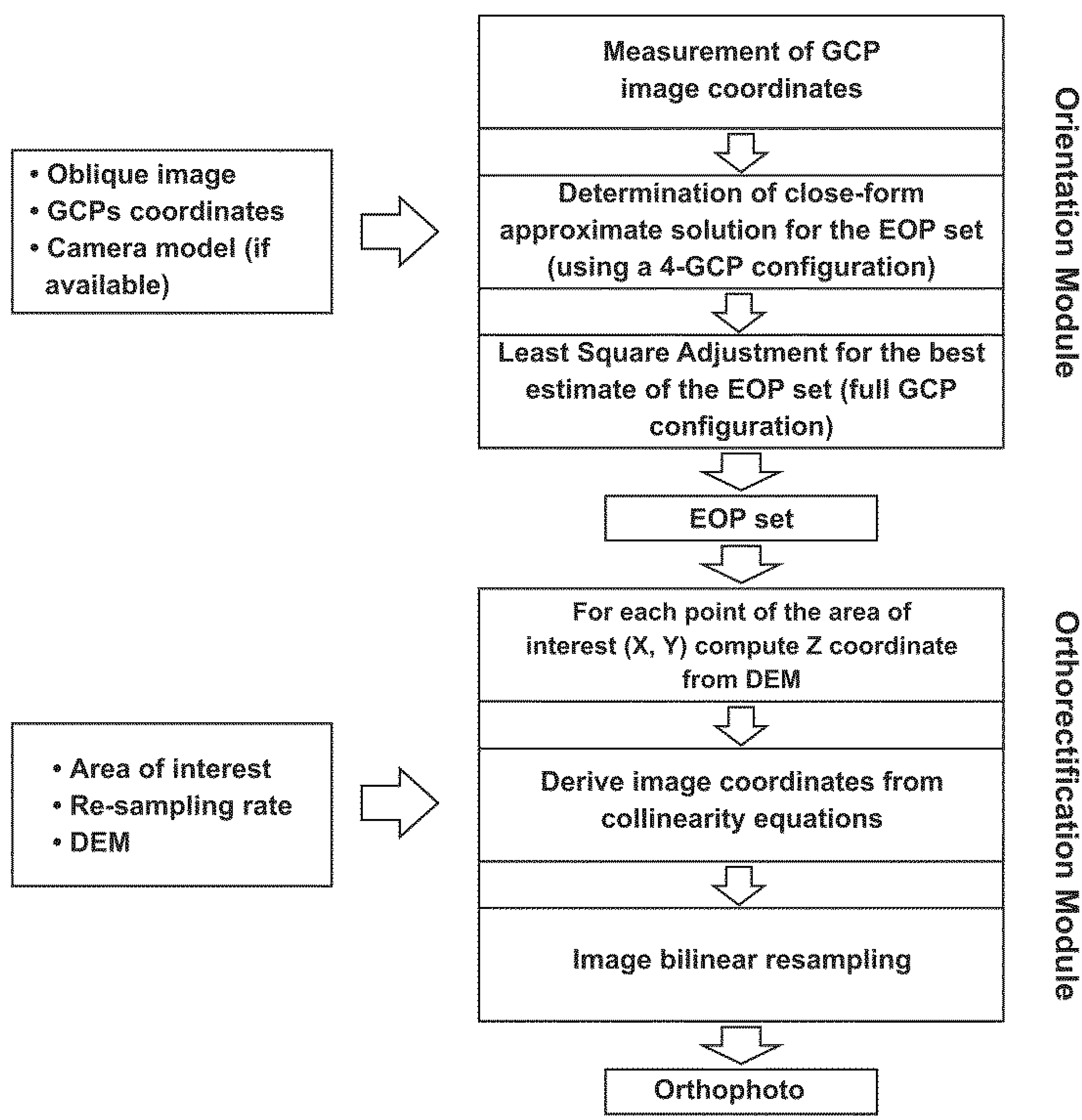
The implemented tool can be divided into two modules (Figure 1) according to their functionalities: an orientation module, which is based on a space resection approach to estimate the external orientation parameters of each image, and an orthorectification module to generate a geometrically corrected and georeferenced raster map, that is a digital orthophoto.

In the first module, the input parameters are the image, a set of GCPs and, if known, the camera model, which would allow for the reduction of the effect of lens distortions, by correcting the image coordinates of GCPs. The outputs are the external orientation parameters, that is the coordinates of the image center and the attitude of the camera at the acquisition time, which are extracted using a Least Square (LS) adjustment and used as input for the second module. In order to evaluate the quality of the estimated solution, standard deviations of the orientation parameters and of the residuals associated to each GCP are also provided.

In the second module, the orthorectification is performed by means of a geometrical transformation from pixel coordinates (x, y) in the Image Reference System (IRF) to the corresponding ground ones (X, Y, Z) in the External Reference System (ERF). The transformation is based on the collinearity equations [17] and on the knowledge of external orientation parameters, estimated in the first module. The elevation value, Z, of each point of the orthophoto is acquired from a reference DEM. A bilinear resampling method is used to define radiometric values g(X, Y) associated to each pixel within the orthophoto. The orthophoto final GSD is defined by establishing a re-sampling rate, accordingly to the image resolution, which may range between 0.8 and 1.2 times the image pixel size multiplied by the mean scale of the image. The orthophoto is provided in standard formats (jpg, tiff, bmp) and relative georeferencing external files (jpw, tfw, bpw). GCP residuals and the associated statistics are stored in ASCII format.

Figure 1. Outline of the algorithms implemented in the Orthoview software: image orientation and image orthorectification modules. EOP stands for External Orientation Parameters.

Figure 1. Outline of the algorithms implemented in the Orthoview software: image orientation and image orthorectification modules. EOP stands for External Orientation Parameters.

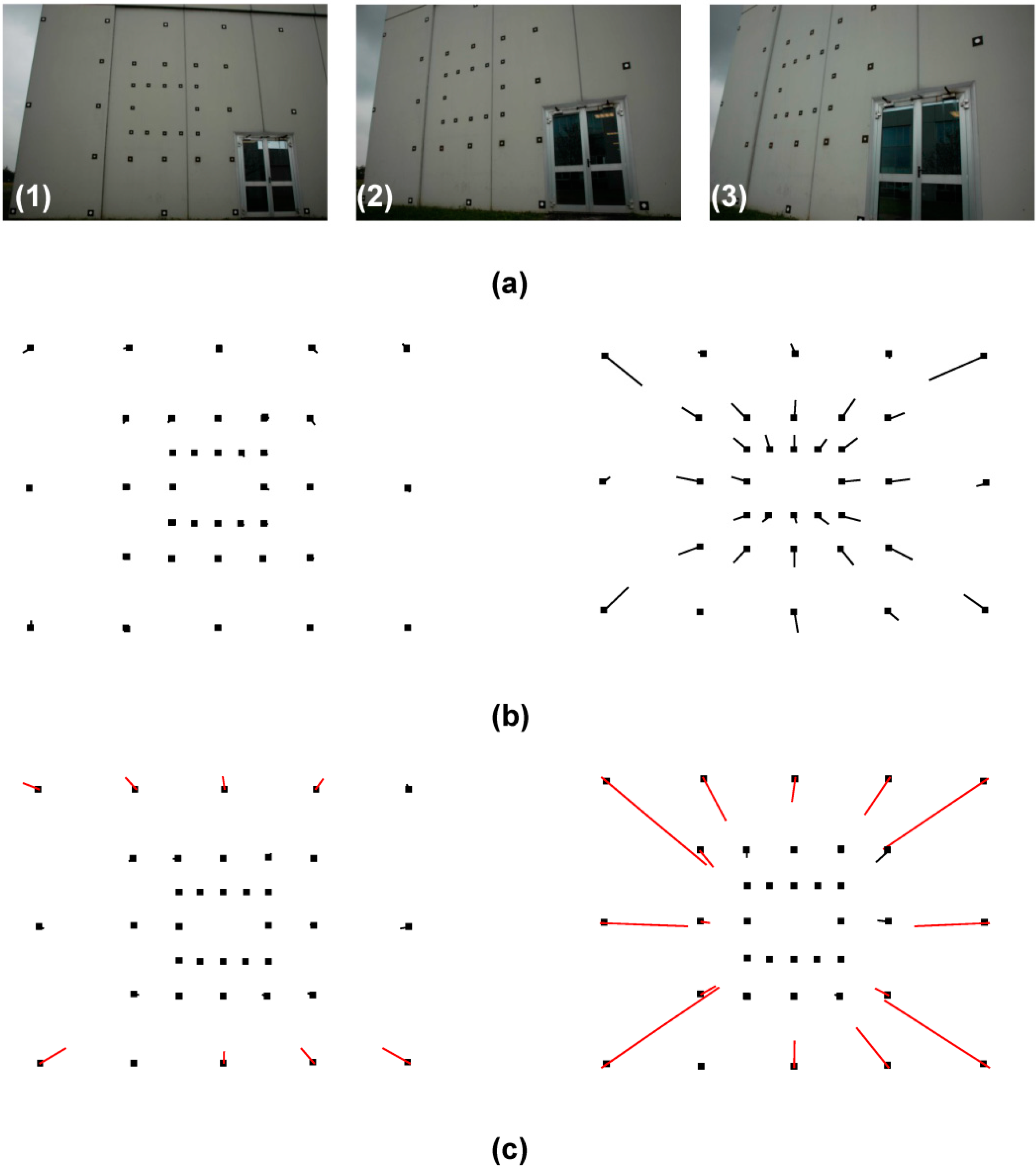
3.2. Calibration Test Field

The influence of the input parameters was assessed by performing a sensitivity analysis on several images acquired, with a Nikon D100 camera, on a calibration test field formed by 36 GCPs whose coordinates were known with an accuracy of few millimeters (Figure 2a). The orientation of each photo was first calculated by a rigorous bundle adjustment performed with the scientific software CALGE [18]. Successively, the influence of camera calibration, the accuracy of the approximate external orientation and the effect of GCP distribution were investigated. Since the calibration test bed is a planar surface, the influence of morphological characteristics and of their uncertainties (DEM and associated errors) was not considered. A further investigation of this aspect with results obtained using data acquired at Etna and Stromboli is described in Section 4.1, Section 4.2, Section 4.3, Section 4.4 and Section 4.5.

Figure 2. (a) Three different views the first of the calibration test field formed by 36 Ground Control Points (GCPs). The tilt of the images increases from left to right; (b) Residuals obtained on the Check Points (CPs), with (left) and without (right) camera distortion correction, by using all the available CPs; (c) Residuals obtained on the CPs, with (left) and without (right) camera distortion correction, by using only the central points.

Figure 2. (a) Three different views the first of the calibration test field formed by 36 Ground Control Points (GCPs). The tilt of the images increases from left to right; (b) Residuals obtained on the Check Points (CPs), with (left) and without (right) camera distortion correction, by using all the available CPs; (c) Residuals obtained on the CPs, with (left) and without (right) camera distortion correction, by using only the central points.

3.2.1. Camera Calibration

If non-calibrated lenses (interior orientation parameters unknown) are used, default parameters corresponding to approximate values of focal length (value declared by the camera brand), Principal Point (PP) coordinates which coincide with the image mid-point (number of rows/2; number of columns/2) and null values for all the distortion parameters, can be applied. It is well known that if we apply such an ideal camera model (pinhole model), without taking into account the calibration parameters (sensor distortion and geometry), we introduce large approximations that cause several errors in the subsequent image processing [19,20] owing to a geometry that is quite different from an ideal central perspective projection.

During camera calibration, the knowledge of the interior parameters (focal length, PP coordinates as well as the three coefficients, K1, K2, K3, of radial distortion and two, P1, P2, of decentering distortion) provides a camera model to correct for geometrical distortions introduced by lens and sensor. There are different approaches to calculate interior parameters. Generally, this calculation is performed with a perspective geometrical model by means of a bundle adjustment approach [19] which considers additional parameters (up to eleven) in the non-linear collinearity equation. A review and a comparative analysis between different approaches are provided in [20]. The camera calibration of the Nikon D100 camera was here obtained using the bundle adjustment software CALGE [18].

The influence of the calibration parameters has been evaluated on the calibration test field by estimating the residuals on the GCPs with and without camera distortion correction. The solution was obtained by using both all the available GCPs (Figure 2b) and only the central points (Figure 2c). The calibration improves the overall results (Figure 2b, left side) by reducing the effects of distortions at the borders of the image that are visible when the camera calibration is neglected (Figure 2c, right side). Considering that GCPs are often located at the border of a photo, it is worthwhile to put additional efforts for estimating sensor calibration parameters.

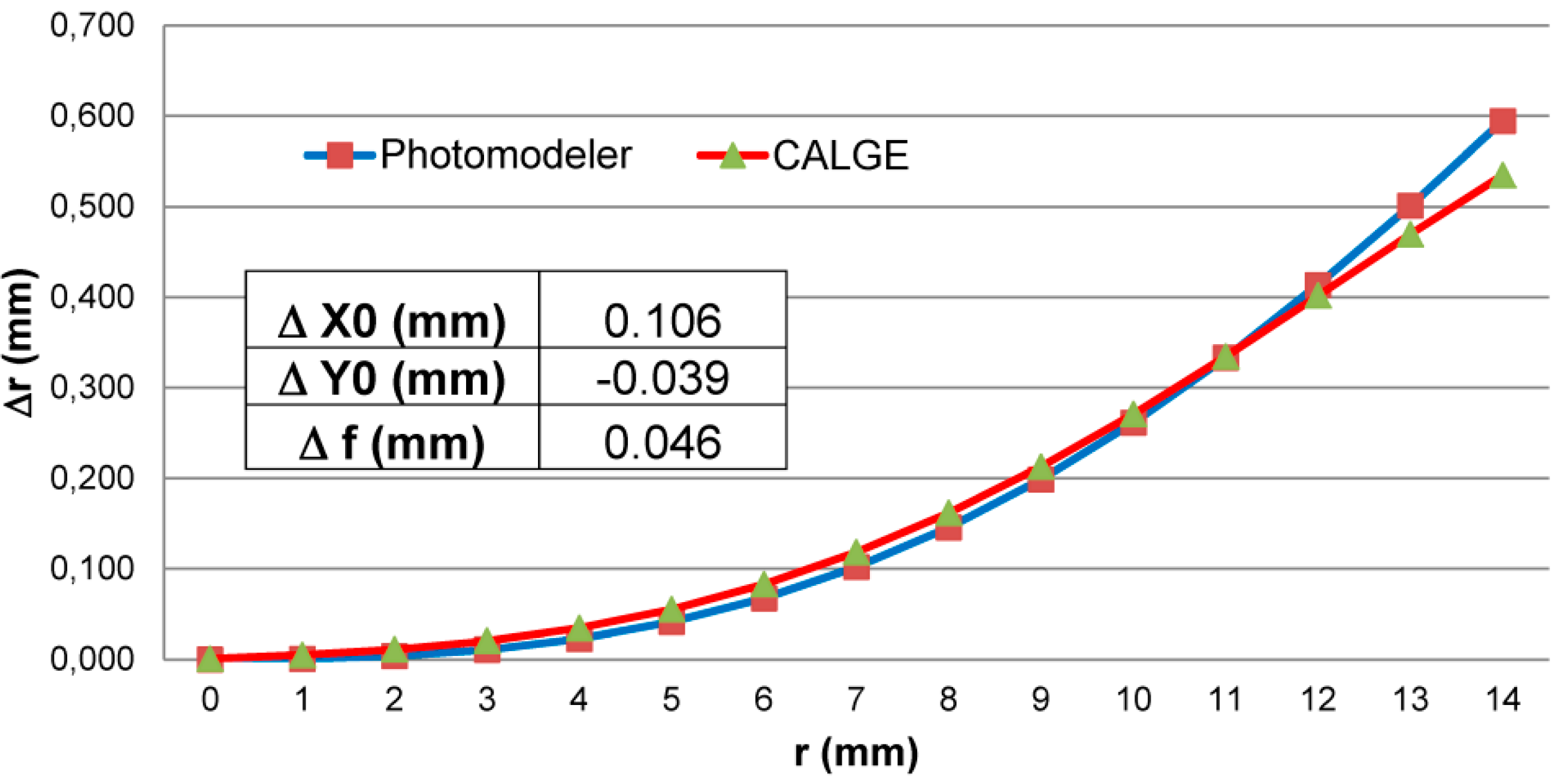
The camera calibration parameters obtained with CALGE [14] were then compared with those evaluated using the procedure implemented in the Photomodeler software [21]. The observed differences for the focal lengths and the PP coordinates (Figure 3) are of the order of tenth of millimeter while the curves of the distortion parameters have differences within 2 pixels (about 15 μm) except at the four corner of the photo (at a distance of 13 mm from the principal point) where the difference increase up to 7 pixels (about 0.05 mm).

Figure 3. Curve of radial distortions evaluated for the Nikon D100 camera using the CALGE (green triangles) and Photomodeler (red squares) software packages. The difference between the PP coordinates and the focal lengths obtained are shown in the embedded table.

Figure 3. Curve of radial distortions evaluated for the Nikon D100 camera using the CALGE (green triangles) and Photomodeler (red squares) software packages. The difference between the PP coordinates and the focal lengths obtained are shown in the embedded table.

3.2.2. Approximate Solution for Space Resection

In order to solve the space resection problem, 4 GCPs are necessary to estimate a unique solution for the 6 parameters defining the external orientation: camera coordinates (X₀, Y₀, Z₀) and attitude angles (ϕ, ω, κ). Moreover, the space resection is a non-linear problem, which must be linearized around approximate values.

Different methods are available to estimate the approximate values in a closed form solution. First to be mentioned is the Direct Linear Transformation (DLT), which is based on at least 6 GCPs because it solves at the same time the interior and external orientation parameters [22]. This method requires redundant GCPs that are well distributed on the photos, which limits the performance of our approach, therefore two alternative solutions were evaluated: the closed form solutions proposed by Zeng [23] and the approach based on quaternions proposed by Sansò [24].

The different algorithms were evaluated on the test field (Figure 2a) through an exhaustive combination of 4-GCP configurations. For each combination, the remaining 32 CGPs were considered as Check Points (CP) to determine the differences between the reference coordinates and the estimated ones. The solution providing the smallest differences was chosen to define the approximate orientation parameters. Table 1 shows the differences between the external parameters calculated by a bundle adjustment software and those estimated by Zeng’s and quaternion methods.

Table 1. Results from images taken on the calibration test field: differences between the external parameters evaluated by a bundle adjustment software and with both Zeng and quaternion approaches applied to the three images in Figure 2. The first column refers to the image number.

	Zeng						Quaternion
	ΔX0 (m)	ΔY0 (m)	ΔZ0 (m)	Δω (deg)	Δφ (deg)	Δκ (deg)	ΔX0 (m)	ΔY0 (m)	ΔZ0 (m)	Δω (deg)	Δφ (deg)	Δκ (deg)
(1)	0.005	−0.003	−0.036	0.135	−0.417	−0.078	−0.043	−0.040	−0.057	0.406	−0.960	−0.968
(2)	0.045	0.182	0.141	12.732	2.630	−1.415	0.061	−0.015	0.088	−1.974	0.717	6.267
(3)	0.122	0.035	−0.045	44.838	30.544	−36.386	0.100	0.019	−0.014	−1.031	0.789	11.377

Table 1. Results from images taken on the calibration test field: differences between the external parameters evaluated by a bundle adjustment software and with both Zeng and quaternion approaches applied to the three images in Figure 2. The first column refers to the image number.

	Zeng						Quaternion
	ΔX0 (m)	ΔY0 (m)	ΔZ0 (m)	Δω (deg)	Δφ (deg)	Δκ (deg)	ΔX0 (m)	ΔY0 (m)	ΔZ0 (m)	Δω (deg)	Δφ (deg)	Δκ (deg)
(1)	0.005	−0.003	−0.036	0.135	−0.417	−0.078	−0.043	−0.040	−0.057	0.406	−0.960	−0.968
(2)	0.045	0.182	0.141	12.732	2.630	−1.415	0.061	−0.015	0.088	−1.974	0.717	6.267
(3)	0.122	0.035	−0.045	44.838	30.544	−36.386	0.100	0.019	−0.014	−1.031	0.789	11.377

The results of Zeng’s algorithm seem to be more influenced by the view geometry, since the all the residuals increase with the image tilt (Figure 2). The quaternion approach provides more steady results for the three configurations, with the exception of the residuals on the k values that increase with the image tilting as well (Table 1).

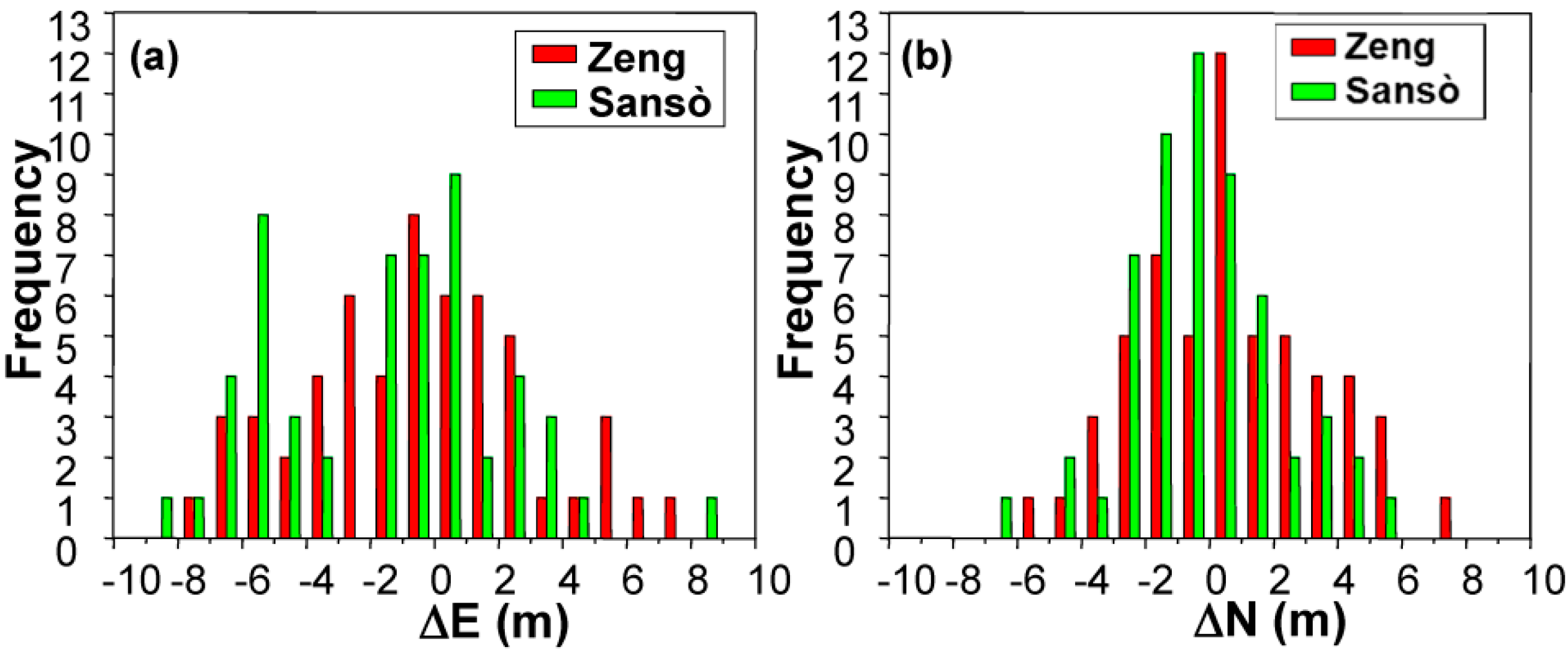
The performance of the Zeng and the quaternion approaches was also evaluated by analyzing the outputs obtained from three photos taken in a real case on Mount Etna. The comparison, based on the difference observed with the East and North coordinates of CPs measured on a reference orthophoto (Figure 4) provided comparable results for the two methods.

Figure 4. Results from images taken on Mt Etna: residuals between the coordinates of Check Points (CP) and those measured of the orthophotos obtained using the Zeng (red bars) and quaternion (green bars) approaches. (a) East coordinates; (b) North coordinates.

Figure 4. Results from images taken on Mt Etna: residuals between the coordinates of Check Points (CP) and those measured of the orthophotos obtained using the Zeng (red bars) and quaternion (green bars) approaches. (a) East coordinates; (b) North coordinates.

3.2.3. Ground Control Point Distribution

Considering that in real cases GCPs are limited in number and not very well-distributed, a further analysis has been performed to understand how different geometrical configurations of GCPs can affect the accuracy of the final results. For example, if the points are clustered in a portion of the image, the solution is ill conditioned and hardly converges. Therefore an image taken on the test field (Figure 2a) was processed by considering twelve different configurations of GCPs with the following characteristics:

• Well distributed GCPs: 36, 24 and 12 points in configurations 1, 2; and 3, respectively;
• Poorly distributed GCPs: 12 points all located in the center of the image for configuration 4; 21 points, on the top and on the right of the image for configurations 5 and 6, respectively; 12 points all located in a corner for configuration 7;
• Few well distributed GCPs for configurations 8 and 9;
• Few sparsely distributed GCPs for configurations 10, 11 and 12.

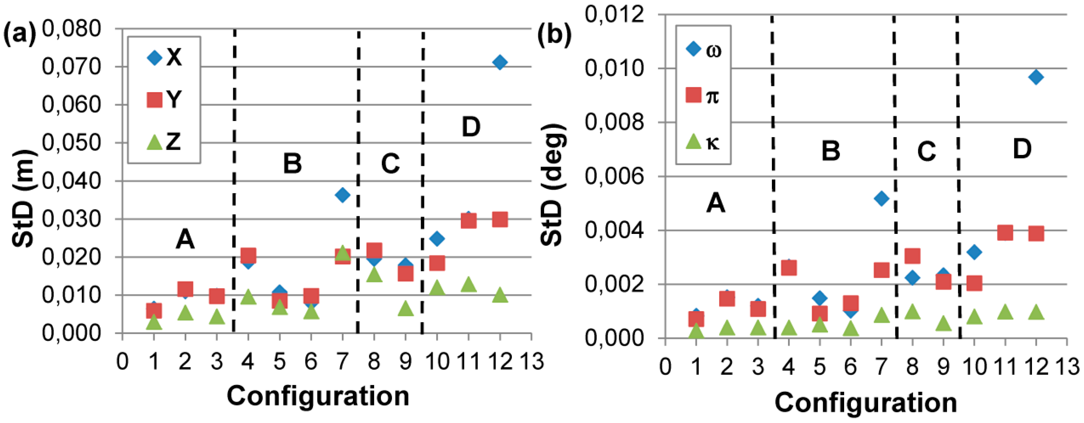
The results obtained in terms of the standard deviation of external orientation parameters, that is on the coordinates of the camera center and on the attitude angles, are summarized in Figure 5. These results shows that even with a low number of well distributed GCPs, surrounding the area of interest (C), a precision in the order of few centimeters can be reached. The algorithm converges to a solution but it is very sensible to GCP distribution.

Figure 5. Sensitivity analysis on the influence of CGP distribution evaluated on the test field showing the standard deviation of the external orientation parameters: camera center coordinates (a) and attitude angles (b) On both figures the dashed lines separate the results relative to the four different classes: (A) well distributed GCPs; (B) poorly distributed GCPs; (C) few well distributed GCPs; (D) few badly placed GCPs.

Figure 5. Sensitivity analysis on the influence of CGP distribution evaluated on the test field showing the standard deviation of the external orientation parameters: camera center coordinates (a) and attitude angles (b) On both figures the dashed lines separate the results relative to the four different classes: (A) well distributed GCPs; (B) poorly distributed GCPs; (C) few well distributed GCPs; (D) few badly placed GCPs.

4. Evaluation of Orthoview Software on Active Volcanic Areas

A number of tests were conducted in active volcanic areas for evaluating the performance of the Orthoview tool and for assessing the effects of operational constraints, such as not-optimal acquisition views and lack of recent maps for measuring GCPs. Recent eruptions of Etna and Stromboli volcanoes were selected as test cases according to the availability of oblique helicopter photos, acquired during or after the active phases, as well as of high resolution reference digital orthophotos and DEMs acquired before the beginning of the eruptions (reference datasets).

The oblique helicopter photos, the pre-eruption DEM and the GCPs coordinates are the input files required by the Orthoview software, while the certificate of camera calibration is an optional input file. Various consumer cameras were used during the different volcanic crisis, thus photos taken by non-calibrated cameras have been used in this study as they represent the only data available for some events. However, as described above, the use of the camera calibration parameters can greatly improve the quality of the output data. Natural points, well visible on the oblique photos, were identified and measured on the pre-eruption orthophotos and DEMs and used as GCPs. The pre-eruption orthophotos and DEMs have also been used for evaluating the accuracy of the Digital Orthophotos (DO) extracted with Orthoview by measuring natural points or features clearly identifiable on both datasets.

The selected test cases include: the Stromboli summit area after the 2002–2003 eruption (Section 4.1); the 2006 Etna eruption (Section 4.2); the 2007 Stromboli eruption (Section 4.3); the 2010 overflow from Stromboli summit area (Section 4.4) and the first Etna paroxysmal eruptive event of 2011 (Section 4.5).

4.1. Test 1: The Stromboli Summit Area after the 2002–2003 Eruption

The first preliminary test was performed to map the summit area of Stromboli volcano after the 2002–2003 eruption, which strongly modified its morphology. A number of images, covering an area of about 1 km², were collected in October 2003 during a helicopter survey using a Nikon D100 camera with 28 mm focal length lens. 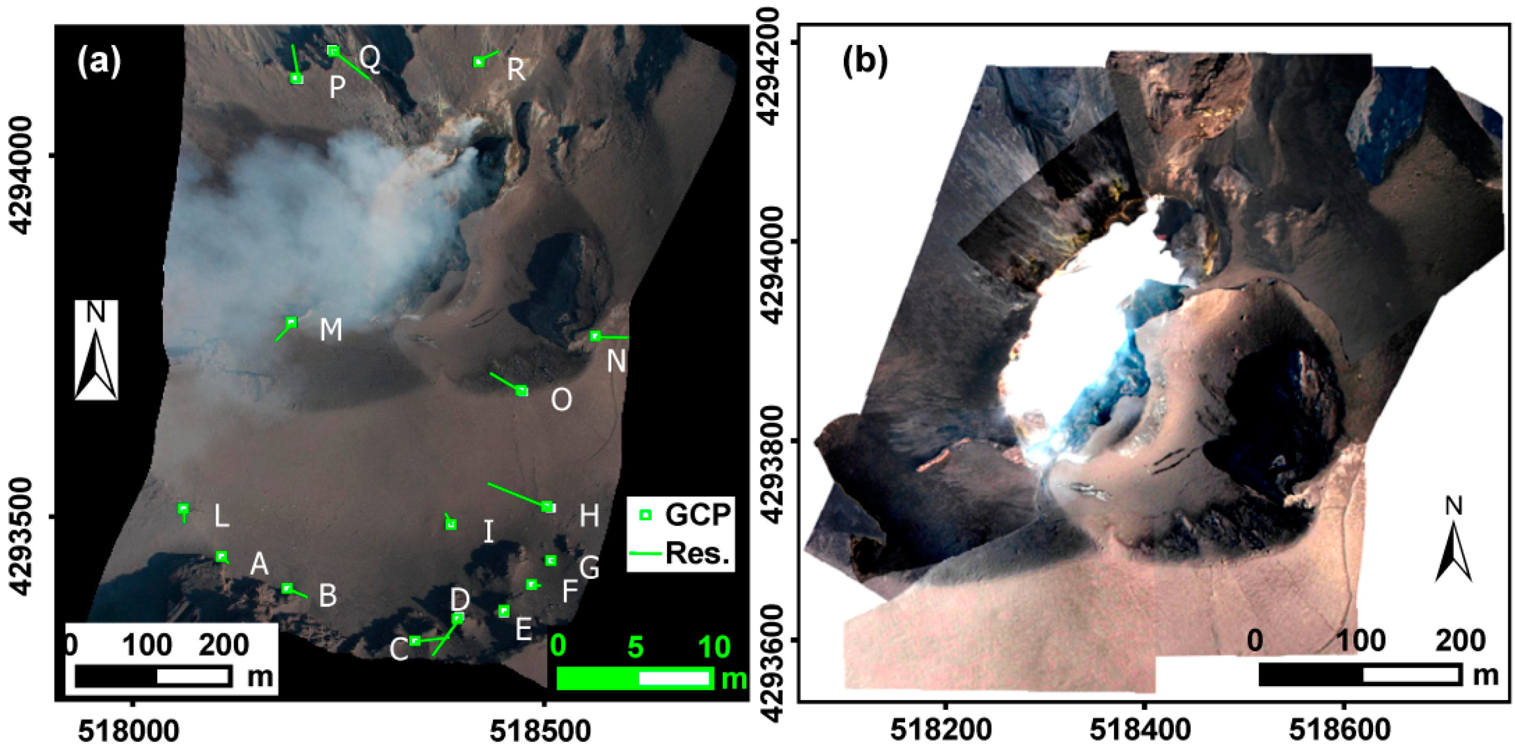GCPs were measured on a 1:5000 aerial photogrammetry dataset obtained in 2001 [1] and are distributed around the crater depression. The different orthophotos were processed and merged to obtain a single orthophoto that covers the whole area at a scale of 1:1000 (Figure 6). The statistics of post adjustment residuals on the GCPs provided mean standard deviations of residuals of ±1.9 m and ±1.3 m on the North and East components, respectively.

Figure 6. Test 1—Stromboli summit area: (a) Orthorectified image acquired on Stromboli crater area after the 2002–2003 eruption showing the residuals (Res.) obtained on the GCPs. The scale bars of the orthorectified image and of the GCP residuals are shown in black and green, respectively; (b) Mosaic of the orthophotos necessary for mapping the whole crater area.

Figure 6. Test 1—Stromboli summit area: (a) Orthorectified image acquired on Stromboli crater area after the 2002–2003 eruption showing the residuals (Res.) obtained on the GCPs. The scale bars of the orthorectified image and of the GCP residuals are shown in black and green, respectively; (b) Mosaic of the orthophotos necessary for mapping the whole crater area.

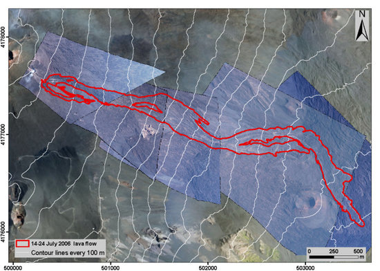
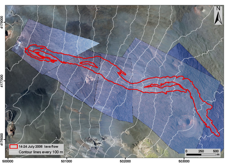
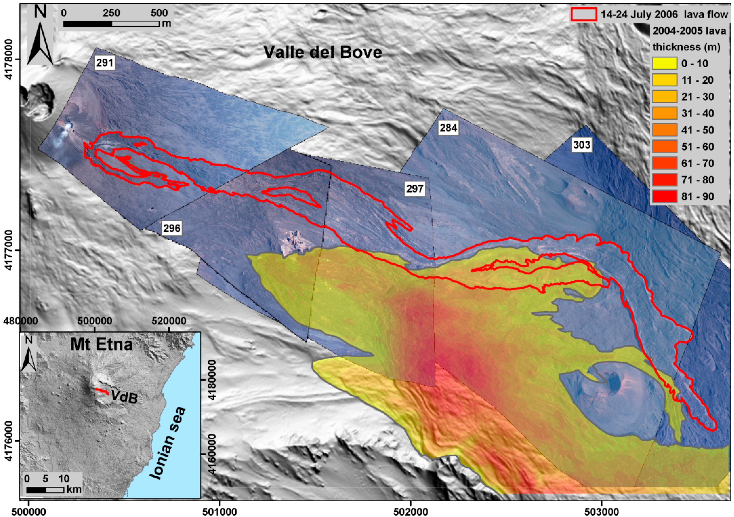
4.2. Test 2: The 14–24 July 2006 Eruption of Mt Etna

The second validation test was conducted using photos taken at Mt Etna from a helicopter and showing a single lava flow, about 4 km long, emplaced inside the Valle del Bove (VdB) between 14 and 24 July 2006. A successive eruptive phase produced a lava flow between 31 August and 14 December 2006, which partially overlapped and expanded the previous ones [25]. Aerial images were acquired on 28 July 2006 to map the first flow, using a Nikon D100 camera with 28 mm focal length lens. The five DOs generated using Orthoview, from the 28 July images, are the only data available for delineating the 14–24 July lava flow (Figure 7).

As reference datasets a pre-eruption DEM (5 m) and a large scale orthophoto (<1 m) generated from aerial surveys in 2005 were adopted [15]. Table 2 reports the external orientation parameters with the associated standard deviations, useful to appraise the errors associated to the measurements that can be done on the relative DO. In addition, the Orthoview software provides post-adjustment residuals, which are the difference between the estimated GPC coordinates and those measured on the reference orthophoto. The standard deviations of post adjustment GCP residuals are reported in Table 3 indicating an overall precision of about 1 m.

Figure 7. Test 2—2006 lava flow in Valle del Bove (Mt Etna): view of orthorectified images showing the limits of the lava flow formed between 14 and 24 July 2006 (red line). The colored map represents the area and the thickness of the 2004–2005 lava field. The inset indicates the location of the 2006 lava flow on the shaded relief image of Etna volcano.

Figure 7. Test 2—2006 lava flow in Valle del Bove (Mt Etna): view of orthorectified images showing the limits of the lava flow formed between 14 and 24 July 2006 (red line). The colored map represents the area and the thickness of the 2004–2005 lava field. The inset indicates the location of the 2006 lava flow on the shaded relief image of Etna volcano.

In order to perform a quality assessment of the measurements that can be done on the DOs, a set of Check Points (CPs) has been measured on the reference orthophoto (map scale of 1:10,000). The statistics of the residuals on the East and North coordinates of the CPs and on the corresponding displacements are reported in Table 4. Such an analysis demonstrates that the generated DOs are characterized by an accuracy of 1–3 m.

Table 2. Test 2—2006 lava flow in Valle del Bove (Mt Etna): standard deviations of the external orientation parameters for the five DOs showing the 2006 Etna lava flow.

Photo ID	Coordinates of Image Center			Camera Attitude
	E (m)	N (m)	H (m)	ω (deg)	φ (deg)	κ (deg)
291	±2.29	±3.01	±2.08	±0.58	±0.59	±0.50
297	±3.70	±3.68	±2.22	±0.74	±0.78	±0.46
296	±2.78	±3.07	±2.24	±0.35	±0.59	±0.42
284	±1.93	±1.79	±1.17	±0.30	±0.30	±0.18
303	±2.59	±2.58	±1.56	±0.43	±0.41	±0.26

Table 2. Test 2—2006 lava flow in Valle del Bove (Mt Etna): standard deviations of the external orientation parameters for the five DOs showing the 2006 Etna lava flow.

Photo ID	Coordinates of Image Center			Camera Attitude
	E (m)	N (m)	H (m)	ω (deg)	φ (deg)	κ (deg)
291	±2.29	±3.01	±2.08	±0.58	±0.59	±0.50
297	±3.70	±3.68	±2.22	±0.74	±0.78	±0.46
296	±2.78	±3.07	±2.24	±0.35	±0.59	±0.42
284	±1.93	±1.79	±1.17	±0.30	±0.30	±0.18
303	±2.59	±2.58	±1.56	±0.43	±0.41	±0.26

Table 3. Test 2—2006 lava flow in Valle del Bove (Mt Etna): statistics of post adjustment residuals of GCPs adopted for extracting each DO: ground resolution (GSD), number of GCPs, standard deviations (StD) on the East and North components.

Photo ID	GSD (m)	GCP n.	StD_E (m)	StD_N (m)
291	0.46	4	0.71	0.11
296	0.44	5	1.12	1.51
297	0.43	6	1.55	1.00
284	0.50	5	0.21	0.34
303	0.43	6	0.59	0.15

Table 3. Test 2—2006 lava flow in Valle del Bove (Mt Etna): statistics of post adjustment residuals of GCPs adopted for extracting each DO: ground resolution (GSD), number of GCPs, standard deviations (StD) on the East and North components.

Photo ID	GSD (m)	GCP n.	StD_E (m)	StD_N (m)
291	0.46	4	0.71	0.11
296	0.44	5	1.12	1.51
297	0.43	6	1.55	1.00
284	0.50	5	0.21	0.34
303	0.43	6	0.59	0.15

Table 4. Test 2—2006 lava flow in Valle del Bove (Mt Etna): statistics of CP residuals on the East (E_CP) and North (N_CP) components and on the computed displacements (Δ_CP): number of measured points (CP n.), minimum, maximum and mean values (Min, Max and Mean), standard deviations (StD).

Photo ID	CP n.	Residual of E_CP (m)				Residual of N_CP (m)				Residual of Δ_CP (m)
		Min	Max	Mean	StD	Min	Max	Mean	StD	Min	Max	Mean	StD
291	21	−5.73	7.51	−1.04	3.75	−4.81	5.44	−0.52	2.33	0.27	8.19	3.80	2.14
296	24	−4.59	5.95	1.25	2.52	−5.95	10.88	0.72	3.33	1.04	11.52	3.55	2.53
297	12	−7.91	−0.97	−3.91	2.73	−2.20	5.96	2.60	2.63	1.61	9.90	5.36	2.67
284	22	−4.09	3.21	−0.14	1.78	−1.56	5.48	2.73	2.21	0.88	5.54	3.63	1.44
302	24	−4.76	4.60	−0.63	1.94	3.71	8.93	5.19	1.39	3.73	9.38	5.56	1.46

Table 4. Test 2—2006 lava flow in Valle del Bove (Mt Etna): statistics of CP residuals on the East (E_CP) and North (N_CP) components and on the computed displacements (Δ_CP): number of measured points (CP n.), minimum, maximum and mean values (Min, Max and Mean), standard deviations (StD).

Photo ID	CP n.	Residual of E_CP (m)				Residual of N_CP (m)				Residual of Δ_CP (m)
		Min	Max	Mean	StD	Min	Max	Mean	StD	Min	Max	Mean	StD
291	21	−5.73	7.51	−1.04	3.75	−4.81	5.44	−0.52	2.33	0.27	8.19	3.80	2.14
296	24	−4.59	5.95	1.25	2.52	−5.95	10.88	0.72	3.33	1.04	11.52	3.55	2.53
297	12	−7.91	−0.97	−3.91	2.73	−2.20	5.96	2.60	2.63	1.61	9.90	5.36	2.67
284	22	−4.09	3.21	−0.14	1.78	−1.56	5.48	2.73	2.21	0.88	5.54	3.63	1.44
302	24	−4.76	4.60	−0.63	1.94	3.71	8.93	5.19	1.39	3.73	9.38	5.56	1.46

Considering that the 2004–2005 lava field inundated the test area and that a pre-eruption DEM (2004) was available, the influence of disregarded elevation changes in the orthorectification process was also investigated. DOs generated using the 2004 DEM were validated by integrating the previously defined set of CPs with additional points located in the modified area, evidenced by the colored map in Figure 7. A comparative analysis was carried out between the two DOs obtained from the photo with ID 297, that covers the largest portion of the modified area (40%) and which is interested by the largest (up to 90 m) vertical topographic changes (Figure 7). Figure 8 summarizes the obtained results: the map of displacement vectors evaluated for the CPs, for both the 2005 and 2004 DOs, with respect to the reference orthophoto (Figure 8a) and a graph that clearly represents how the magnitude of the displacements increases as a function of the height variation (Figure 8b). A further analysis on the effects of the use of not up-to-date DEM was performed to evaluate the errors associated to the measurement of the area inundated by lava flows, which represents a key parameter for prompt hazard assessment (Figure 8c). A major discrepancy (underestimation of about 46%) has been observed between the most accurate area, measured on the reference orthophoto, and that evaluated on the 2004_DO. A minor discrepancy (underestimation of about 8%) characterizes the 2005_DO, obtained using the up-to-date DEM. This demonstrates that, in order to obtain lava-flow maps with accuracy adequate for short-term monitoring purposes it is convenient, after an eruption and especially after a large one, to carry out topographical surveys for DEM updating.

Figure 8. Test 2—2006 lava flows in Valle del Bove (Mt Etna): (a) Displacement vectors of CPs measured on the DO with ID 297 obtained using the 2005 DEM and the 2004 DEM (red and black arrows, respectively). The yellow line indicates the area covered by the 2004–2005 lava field; (b) Graph showing the magnitude of the displacements in the modified area as a function of the height variations; (c) Comparison between flow limits drawn on the reference orthophoto (yellow), as well as on the 2005 and 2004 DOs (red and black, respectively).

Figure 8. Test 2—2006 lava flows in Valle del Bove (Mt Etna): (a) Displacement vectors of CPs measured on the DO with ID 297 obtained using the 2005 DEM and the 2004 DEM (red and black arrows, respectively). The yellow line indicates the area covered by the 2004–2005 lava field; (b) Graph showing the magnitude of the displacements in the modified area as a function of the height variations; (c) Comparison between flow limits drawn on the reference orthophoto (yellow), as well as on the 2005 and 2004 DOs (red and black, respectively).

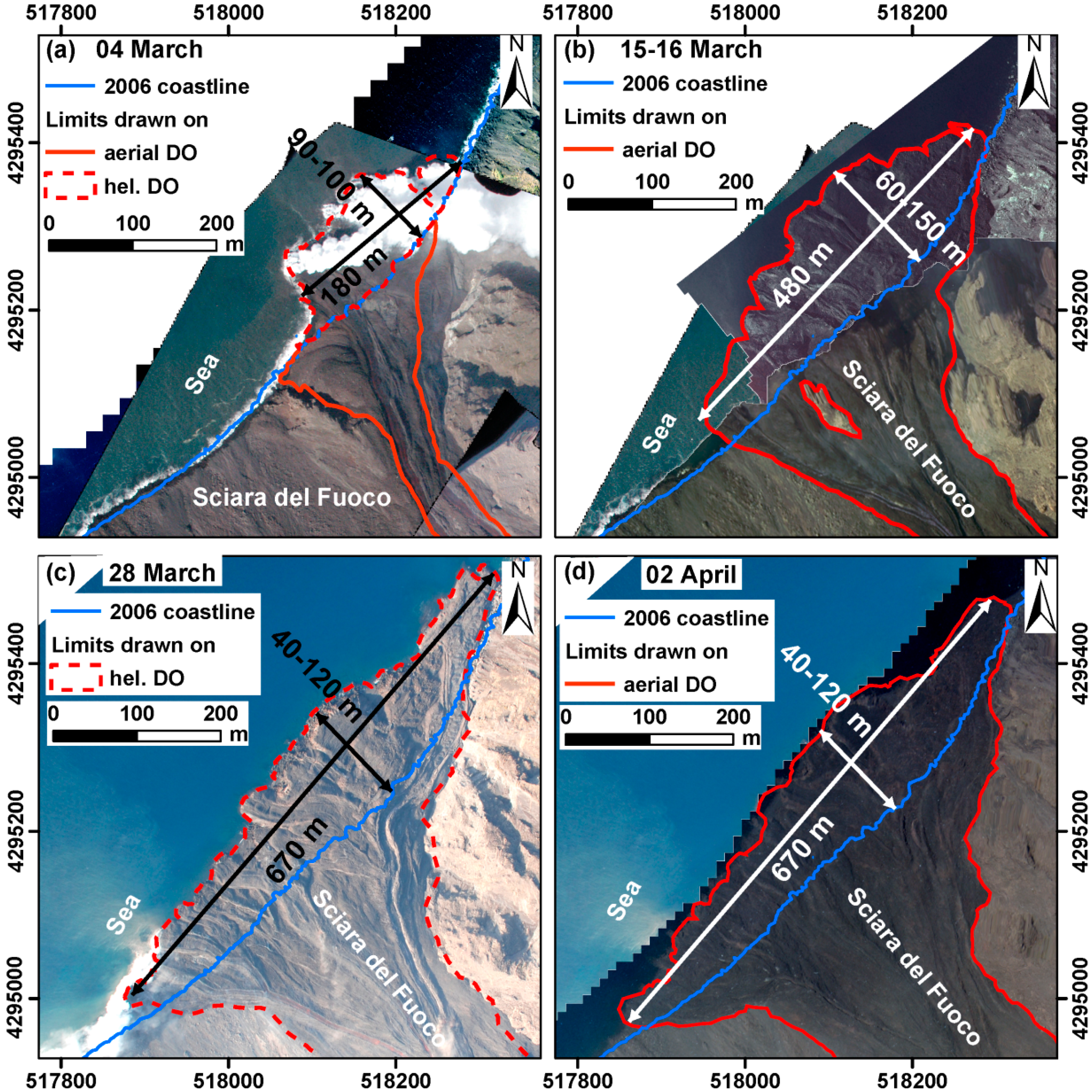
4.3. Test 3: The Sciara del Fuoco Slope during the 2007 Stromboli Eruption

During the 2007 eruption of Stromboli many photos were taken from helicopter using a calibrated Nikon D100 camera with 18 mm focal length lens, to map the evolution of the active lava flows on the Sciara del Fuoco (SdF) slope. The eruption lasted from 27 February until 2 April emitting lava from multiple vents and resulting in a compound lava field that reached the sea forming a fan that rapidly expanded. Periodical photogrammetric and LIDAR aerial surveys were performed to monitor the topographic changes caused by the eruption, while photos from helicopter were acquired almost daily [13]. The available data permitted to extract digital orthophotos and DEMs for evaluating the dimensions and volumes of the lava-flow field. Some of the orthophotos were extracted from the helicopter images using Orthoview, in order to obtain more frequent mapping data (Figure 9). This activity provided useful information on the evolution of the lava fan that overloaded the slope at the coastline level and that, in case of sudden bench collapse, represented a potential hazard for the SdF slope stability.

Figure 9. Test 3—2007 eruption, Stromboli: temporal evolution and dimensions of the fan produced by the main lava flow. (a) 04 March; (b) 15–16 March; (c) 28 March; (d) 2 April. The pre-eruption coastline (2006) is drawn in blue, continuous and dashed lines are limits drawn on an aerial and a helicopter (hel.) DOs, respectively.

Figure 9. Test 3—2007 eruption, Stromboli: temporal evolution and dimensions of the fan produced by the main lava flow. (a) 04 March; (b) 15–16 March; (c) 28 March; (d) 2 April. The pre-eruption coastline (2006) is drawn in blue, continuous and dashed lines are limits drawn on an aerial and a helicopter (hel.) DOs, respectively.

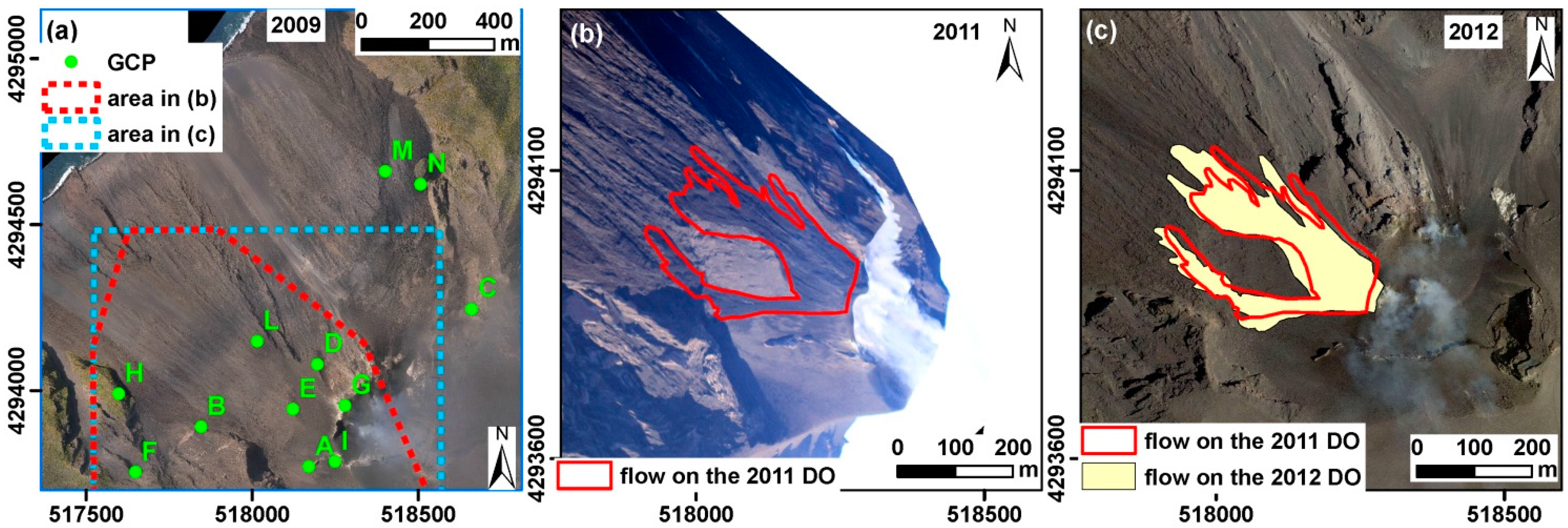
4.4. Test 4: The December 2010 Stromboli Overflow

In December 2010, an increase of the effusive activity caused a lava overflow from the main crater of Stromboli that rapidly flowed along the SdF. It was not possible to perform a helicopter survey until 25 January 2011 when images were taken with a Canon EOS 7D. The DOs generated with Orthoview are shown in Figure 10. An ALS dataset, acquired in 2009, was used as reference for topographic correction and for identifying 11 GCPs (Figure 10a). The lava-flow delineation on the DOs (Figure 10b) allowed the measurements of the maximum lava flow length (~370 m) and the distance of the front from the coastline (~590 m a.s.l.). In addition, average lava thicknesses were estimated by dividing the lava field (~42,700 m²) into three zones based on their average slope. The results of this analysis provided a total lava volume of about 63,500 m³ and an average thickness of 1.4 m.

The first LIDAR aerial survey, useful for delimiting with known accuracy the December 2010 overflows and thus checking the measurements obtained from the January 2011 DOs, was performed by Italian Department of Civil Protection (DPC) in 2012, about 18 months later. The comparison between the two flow field limits shows that the overall geometry of the lava-flow field was well sketched out on the DOs, although the most advanced lava front was approximately 70 m (16%) shorter than the 2012 one (Figure 10c). Moreover, the flow field area was underestimated of about 15% with respect to the one measured using the 2012 dataset.

Figure 10. Test 4—2010 overflow at Stromboli: (a) 2009 orthophoto of Sciara del Fuoco slope and natural points selected as GCPs; (b) Limits of the December 2010 overflow defined on 25 January 2011 DOs; (c) Limits of the December 2010 overflows defined on the on the 2011 DOs (red line) and on the 2012 (yellow polygon), the background image is the 2012 orthophoto.

Figure 10. Test 4—2010 overflow at Stromboli: (a) 2009 orthophoto of Sciara del Fuoco slope and natural points selected as GCPs; (b) Limits of the December 2010 overflow defined on 25 January 2011 DOs; (c) Limits of the December 2010 overflows defined on the on the 2011 DOs (red line) and on the 2012 (yellow polygon), the background image is the 2012 orthophoto.

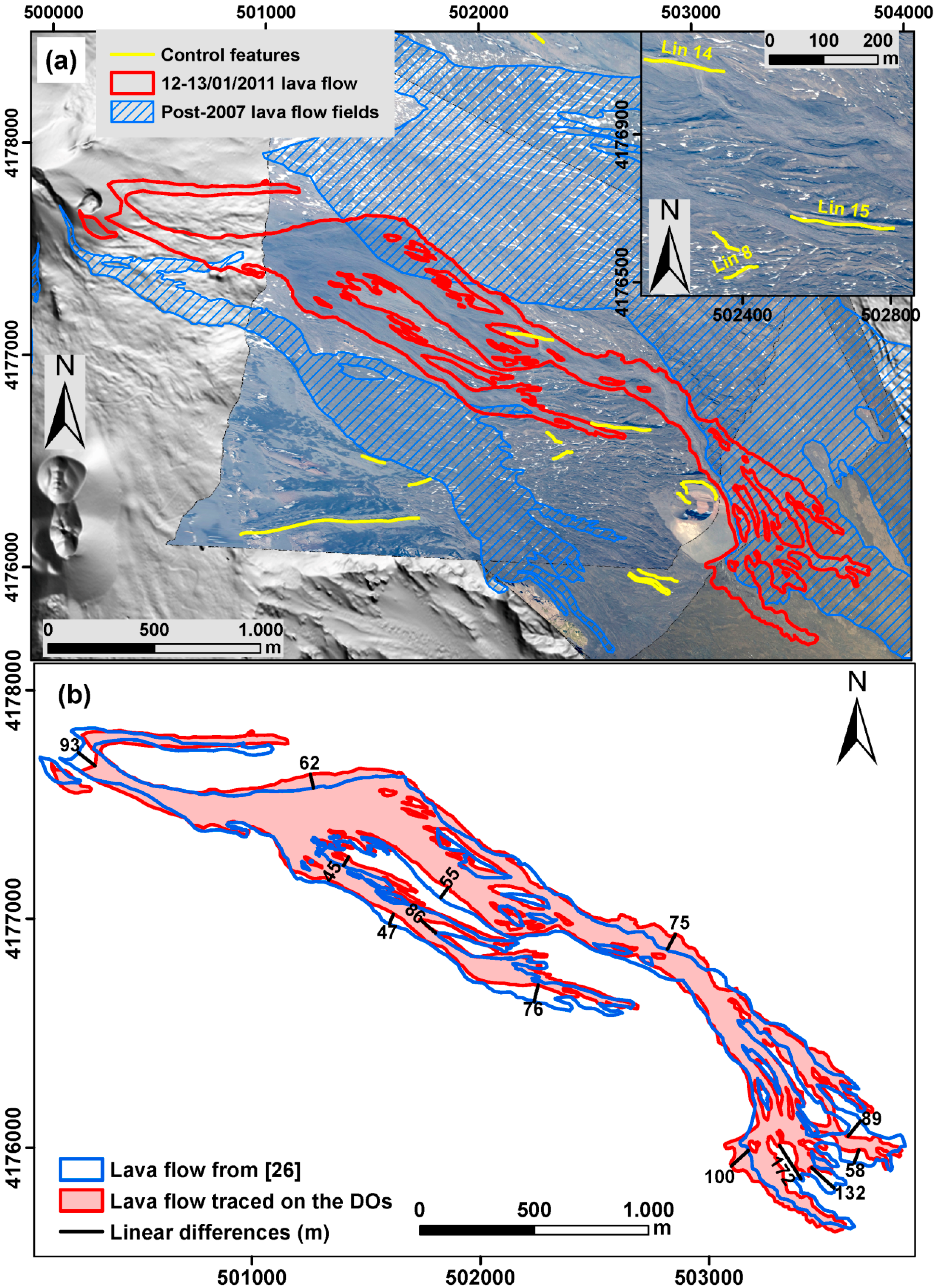
4.5. Test 5: The 12–13 January 2011 Etna Paroxysmal Event

The last test was conducted for the Etna lava flow emplaced in Valle del Bove during a paroxysmal eruptive event occurred on 12–13 January 2011. Images were collected, on 19 January 2011, using a Nikon D90 camera having a 50 mm focal length. In order to minimize scale distortion and occlusions the images were taken in nadir direction. GCPs were measured on a reference orthophoto (sub-meter resolution) and DEM (10 m) acquired in 2005 and 2007, respectively [15].

In order to map the whole lava-flow field, three images were orthorectified. Their accuracy was evaluated by considering the discrepancy between well identifiable linear morphological features measured on the 2011 DO and on the 2005 reference orthophoto (Figure 11a). The statistic associated to distances computed between points selected every 5 m along the polyline drawn on the 2011 DO and the corresponding polyline traced on the 2005 orthophoto are shown in Table 5. The results demonstrate that uncertainties of few meters can be associated to a linear feature measurement, which is acceptable for a rapid mapping of lava flows during emergency phases.

In addition, it was possible to evaluate the accuracy improvements with respect to the not rigorous, but commonly used, approach of drawing the lava limits on existing maps by means of photo interpretation and direct field observations [26]. The comparison showed that the linear differences range between 45 and 75 m in the central portion of the flow field, while they increase up to about 170 m in the frontal area (Figure 11b). In this case, the incorrect location of the lava fronts could have represented a critical issue impacting on hazard evaluation.

Figure 11. Test 5—2011 lava flow in Valle del Bove (Mount Etna): (a) Limits of the 12–13 January 2011 lava flow (red line) drawn on the 19 January 2011 DOs, and areas not up-to-date in the 2007 reference DEM (i.e., 2007–2010 lava flows, dashed polygons). Yellow lines indicate the morphological features used for accuracy evaluation; the inset shows a detail of some features (b) Comparison between the lava-flow field traced on the DOs (red) and that one drawn from direct field observations and photo interpretation (blue line, from [26]).

Figure 11. Test 5—2011 lava flow in Valle del Bove (Mount Etna): (a) Limits of the 12–13 January 2011 lava flow (red line) drawn on the 19 January 2011 DOs, and areas not up-to-date in the 2007 reference DEM (i.e., 2007–2010 lava flows, dashed polygons). Yellow lines indicate the morphological features used for accuracy evaluation; the inset shows a detail of some features (b) Comparison between the lava-flow field traced on the DOs (red) and that one drawn from direct field observations and photo interpretation (blue line, from [26]).

Table 5. Test 5—2011 lava flow in Valle del Bove (Mount Etna): statistics on the distance between natural linear features measured on the 19 January 2011 DOs and on the 2005 orthophoto: number of measured lines (LN n.), number of point along the 2011 linear features (PT n.), line (LN) length, mean and median (Med) values as well as standard deviations (StD) of point-line distances.

Photo ID	LN n.	PT n.	LN Length (km)	Mean (m)	Med (m)	StD (m)
318	8	328	1.64	1.26	0.56	8.97
321	16	496	2.48	7.02	6.95	4.27
331	8	333	1.67	3.19	2.74	2.88
All images	18	1156	5.79	4.28	3.63	6.26

Table 5. Test 5—2011 lava flow in Valle del Bove (Mount Etna): statistics on the distance between natural linear features measured on the 19 January 2011 DOs and on the 2005 orthophoto: number of measured lines (LN n.), number of point along the 2011 linear features (PT n.), line (LN) length, mean and median (Med) values as well as standard deviations (StD) of point-line distances.

Photo ID	LN n.	PT n.	LN Length (km)	Mean (m)	Med (m)	StD (m)
318	8	328	1.64	1.26	0.56	8.97
321	16	496	2.48	7.02	6.95	4.27
331	8	333	1.67	3.19	2.74	2.88
All images	18	1156	5.79	4.28	3.63	6.26

4.6. Discussion of the Results

The test performed using the photos acquired on Stromboli summit area after the 2002–2003 eruption (Test 1) represents the first application of the Orthoview software on an active volcano and it demonstrates its capability of extracting orthophotos, with sufficient accuracy, from oblique aerial images. These data were useful for obtaining quantitative measurements of volcanic landscape features in absence of aerial surveys dedicated to map production.

On Mt Etna, the images taken during the 14–24 July 2006 eruption (Test 2) are the only data available for mapping this lava flow, since it was soon covered by the subsequent effusive activity. Similarly, the helicopter DOs were the only data available in short times for the 2007 Stromboli eruption on the Sciara del Fuoco slope (Test 3) and for the December 2010 Stromboli overflow (Test 4). In the first case, the helicopter DOs were used for more frequently mapping the lava-flow field and for measuring the dimension of the lava delta with sufficient accuracy; in the second case, helicopter DOs furnished the final dimensions of the overflow. Finally, the lava flow produced during the 12–13 January 2011 Etna paroxysmal event (Test 5) was partially covered by lava emitted during the subsequent paroxysmal event occurred on 18 February 2011 [27], only one month after the helicopter survey, which is the only available dataset for mapping the first flow.

Test 5 allowed also to compare the lava-flow field traced on the DOs with that one drawn from direct field observations and photo interpretation [26]. The drawing of the lava limits by means of photo interpretation can result in an inaccurate delimitation of the flow field and to a significant error on the location of the flow fronts thus impacting on the hazard evaluation. The relative small difference (from a few tens of meters up to two hundred meters) can furnish a sufficient low uncertain on the area and volume estimations only for short-lasting eruptions. In contrast, in case of a long-lasting eruption many horizontal errors may cumulate causing final large errors in area and volumes, barely after a few days from the eruption start.

To provide a comparative overview of the performed tests, that use both calibrated and not calibrated sensors, the standard deviations of the external orientation parameters and of the GCP residuals, after outlier removal, are reported in Table 6. This comparison demonstrated that similar results have been obtained when using the same not-calibrated sensor in different areas having different morphologies, i.e., the Stromboli summit area (Test Case, TC 1) and the 2006 Etna lava flow in Valle del Bove (TC 2). Even if the use of calibrated lenses improve the results, as demonstrated for the calibration test-field (see paragraph 3.2.1), this enhancement is not evident in the tests performed on volcanic areas: comparable results were obtained both when using calibrated (TC 3) and not calibrated lenses (TCs 1 and 2). The use of natural instead of signalized GCPs, thus characterized by lower accuracy, introduce errors of large magnitudes that can hide the benefit deriving by the correction of the error linked to image distortion.

Table 6. Evaluation of the software performance: Test Cases (TC) numbered as in paragraph 4; Internal Orientation Parameters (IOP), Not-Available (NA) or Available (A); number (n.) of PDO for each test; ground resolution (GSD); number of GCP (GCP n.); Standard Deviation (StD) of GCP residuals: and Standard Deviation of External Orientation Parameters (StD of EOP). Average values on all the PDOs are reported for each test.

TC	IOP	PDO n.	GSD (m)	GCP n.	StD of EOP						StD GCP res.
					X (m)	Y (m)	Z (m)	ω (deg)	φ 3 (deg)	κ (deg)	E (m)	N (m)
1	NA	4	0.30	8	2	2	1	0.58	0.45	0.33	1	2
2	NA	5	0.45	5	3	3	2	0.48	0.53	0.36	1	1
3	A	3	0.28	4	3	3	3	0.99	0.77	0.52	2	2
4	NA	1	0.21	4	10	12	12	2.00	2.24	1.61	4	4
5	NA	3	0.37	4	6	4	6	0.71	0.69	0.62	2	4

Table 6. Evaluation of the software performance: Test Cases (TC) numbered as in paragraph 4; Internal Orientation Parameters (IOP), Not-Available (NA) or Available (A); number (n.) of PDO for each test; ground resolution (GSD); number of GCP (GCP n.); Standard Deviation (StD) of GCP residuals: and Standard Deviation of External Orientation Parameters (StD of EOP). Average values on all the PDOs are reported for each test.

TC	IOP	PDO n.	GSD (m)	GCP n.	StD of EOP						StD GCP res.
					X (m)	Y (m)	Z (m)	ω (deg)	φ 3 (deg)	κ (deg)	E (m)	N (m)
1	NA	4	0.30	8	2	2	1	0.58	0.45	0.33	1	2
2	NA	5	0.45	5	3	3	2	0.48	0.53	0.36	1	1
3	A	3	0.28	4	3	3	3	0.99	0.77	0.52	2	2
4	NA	1	0.21	4	10	12	12	2.00	2.24	1.61	4	4
5	NA	3	0.37	4	6	4	6	0.71	0.69	0.62	2	4

5. Conclusions

The problem of keeping geological maps up-to-date is a quite demanding issue, especially for very active volcanoes like Etna and Stromboli [28,29], where frequent eruptions produce large changes of the landscape. The standard aerial photogrammetric approach is one of the most effective techniques for mapping fast evolving natural phenomena, despite of the fact that dedicated airborne systems are not always available due to the operational constrains. The frequency of data acquisition can be increased by utilizing imagery acquired during helicopter surveys, quite frequently performed throughout volcanic crises. In order to take advantage of helicopter surveying for rapid mapping purposes, it is necessary to adopt a simplified procedure for processing imagery that do not meet the requirements of vertical photogrammetry.

This work discusses the results obtained by using a software, i.e., Orthoview, developed for processing oblique single-view acquisitions that was tested on active volcanic areas. The study highlights that the accuracy of the produced maps depends on the quality of GCPs, which in areas difficult to access often correspond to natural features, and on the quality of the DEM used for image projection. However, the mapping accuracy achievable on 2D features, measured on the orthophoto maps, is considered adequate to assess hazard scenarios, in particular by permitting to rapidly establish the position and the rate of advancement of the lava fronts along the volcano slopes.