Automatic Seamline Network Generation for Urban Orthophoto Mosaicking with the Use of a Digital Surface Model

Abstract

Intelligent seamline selection for image mosaicking is an area of active research in the fields of massive data processing, computer vision, photogrammetry and remote sensing. In mosaicking applications for digital orthophoto maps (DOMs), the visual transition in mosaics is mainly caused by differences in positioning accuracy, image tone and relief displacement of high ground objects between overlapping DOMs. Among these three factors, relief displacement, which prevents the seamless mosaicking of images, is relatively more difficult to address. To minimize visual discontinuities, many optimization algorithms have been studied for the automatic selection of seamlines to avoid high ground objects. Thus, a new automatic seamline selection algorithm using a digital surface model (DSM) is proposed. The main idea of this algorithm is to guide a seamline toward a low area on the basis of the elevation information in a DSM. Given that the elevation of a DSM is not completely synchronous with a DOM, a new model, called the orthoimage elevation synchronous model (OESM), is derived and introduced. OESM can accurately reflect the elevation information for each DOM unit. Through the morphological processing of the OESM data in the overlapping area, an initial path network is obtained for seamline selection. Subsequently, a cost function is defined on the basis of several measurements, and Dijkstra’s algorithm is adopted to determine the least-cost path from the initial network. Finally, the proposed algorithm is employed for automatic seamline network construction; the effective mosaic polygon of each image is determined, and a seamless mosaic is generated. The experiments with three different datasets indicate that the proposed method meets the requirements for seamline network construction. In comparative trials, the generated seamlines pass through fewer ground objects with low time consumption.

1. Introduction

1.1. Background

The growing demand for richer information and better visual experience in a single image has caused the increasing application of seamless image mosaicking in scientific domains, such as massive data processing, computer vision, photogrammetry and remote sensing. In remote sensing, this technique is applied to different datasets, including satellite [1,2,3], aerial [4,5,6,7], low-altitude [8,9] and close-range [10,11] images. In a typical processing pipeline, aerial images are always reprojected onto a digital terrain model (DTM) with various camera locations and orientations, and the obtained digital orthophoto maps (DOMs) are used for mosaicking [12]. Thus, generating mosaics from DOMs has attracted considerable attention.

The most important idea of image mosaicking is combining two or more images into a larger image with minimal visual transition. When applying mosaicking to high-resolution urban DOMs, visual transition is mainly caused by three aspects among images: positioning accuracy, tone and relief displacement of high ground objects. Positioning accuracy can be improved through high-quality bundle block adjustment, whereas tone differences can be addressed by image color balancing and feathering [13]. However, relief displacement is relatively more difficult to address in mosaicking. Relief displacement mainly occurs because a DTM does not contain elevations for ground objects, such as buildings and bridges, thus causing the imperfect rectification of such objects in DOMs. Figure 1a,b shows the relief displacements of the same building in different directions. These displacements result from imaging from different angles. When the seamline of the mosaic passes through the building in Figure 1c, a significant visual discontinuity occurs.

An ideal solution is the use of true DOMs (TDOMs) rectified with a digital surface model (DSM) for mosaicking. However, although TDOMs theoretically have no relief displacement, the automatic generation of TDOMs involves many complex technical procedures, such as shadow detection, restoration, occlusion detection and compensation [14]. A high-quality DSM is insufficient to create a satisfactory TDOM, because automatic production is still immature. Another method is selecting the seamline for DOMs through human interaction, but manual intervention may become inappropriate when processing with sizable data. Thus, scholars study automatic algorithms for seamline optimization and attempt to select the seamline in areas where no obvious ground objects appear on two overlapping DOMs, thus minimizing visual discontinuities.

Figure 1. Visual discontinuity caused by relief displacement. (a) A building is provided in a digital orthophoto map (DOM); (b) the same building is provided in another DOM, where the original image is captured from a different angle; (c) the building is provided in the mosaicked image of two overlapping images, where the red line indicates the randomly selected seamline.

Figure 1. Visual discontinuity caused by relief displacement. (a) A building is provided in a digital orthophoto map (DOM); (b) the same building is provided in another DOM, where the original image is captured from a different angle; (c) the building is provided in the mosaicked image of two overlapping images, where the red line indicates the randomly selected seamline.

1.2. Related Works

A typical automatic seamline selection algorithm is developed by estimating the pixel-by-pixel differences in overlapping image areas. First, a cost function is created on the basis of one or more measurements, and then, a least-cost path is defined as the best seamline through several searching methods. In one of the first published algorithms, the gray level difference is determined as the measurement [15]. Given that the difference only reflects changes in a single pixel without neighborhood information, image gradient difference [16,17] and normal cross-correlation [18,19] were selected as measurements in succeeding research. Moreover, in some approaches, image edges [2], salient features [20] and distance to nadir points [20,21] are also considered for seamline optimization. As regards the least-cost path searching algorithms, path optimization methods based on Dijkstra’s algorithm are commonly used [10,22,23,24,25]. Meanwhile, numerous algorithms perform well in seamline searching. These algorithms include the snake technique [26], bottleneck model [5,6,12], dynamic programming [20], ant colony [18] and Floyd–Warshall [27].

The overlapping area between two images can be sizable (such as that between aerial images with large overlap), indicating that the least-cost path should be determined in a search space of millions of pixels. The enormous amount of computation becomes unbearable when constructing a seamline network for a large survey area. Thus, one approach to reduce computation is to create an initial seamline on the basis of simple topological relationships, such as the Voronoi diagram, and then performing optimization within a certain range from the initial seamline [12,28]. Another approach is to remove the unwanted areas in the overlap through threshold adjustment [19] or image segmentation [25], after which the least-cost path is determined in a restricted sub-area. Both approaches somehow improve efficiency.

Most seamline selection algorithms are developed on the basis of image gray information analysis. However, gray information has limited reliability. Thus, determined seamlines may still pass through some high objects when faced with insufficient texture or uneven tone. Hence, some scholars study seamline selection using external data.

Wan et al. [24,27] attempted to use existing vector roads to generate seamlines. In their research, the vector roads in the overlapping area are overlaid with an extracted skeleton to create a weighted graph, and the least-cost path is selected as the seamline on the basis of this graph. Seamlines away from most high ground objects can be selected on the basis of road information, and computational complexity is considerably decreased. However, automatically obtaining reliable vector road data could be difficult, and manual mappings are always required to produce the vector data.

Ma et al. [29] used point cloud data from the light detection and ranging (LiDAR) system to identify high ground objects as obstacles and attempted to guide seamlines to avoid these obstacles. The results exhibit an improvement in both efficiency and quality with the use of LiDAR data. However, for ground objects with relief displacement, the elevation from LiDAR is asynchronous with the same object in a DOM (see the analysis in Section 2.1). Given the influence of these deviations, the seamline generated with the LiDAR data can theoretically pass through the ground object.

1.3. Proposed Approach

A new automatic seamline selection algorithm using DSM data is proposed in this study. Given that a DSM elevation is not completely synchronous with that of a DOM, a new model, called an orthoimage elevation synchronous model (OESM), is derived and introduced [30]. In an OESM, the elevation of an object in a DOM becomes accordant with the actual height of the same object in a DSM, even in areas where relief displacement occurs. In our approach, an OESM is successfully applied to the seamline network construction of DOMs for the first time. First, a series of morphological processing steps is performed for the OESM data in the overlapping area, and an initial path network is obtained for seamline selection. Second, a cost function is defined on the basis of measurements, including the total path length, original path width and distance from the node to the skeleton. Dijkstra’s algorithm is adopted to determine the least-cost path. Finally, the new seamline selection method is employed for automatic seamline network construction. The effective mosaic polygon (EMP) of each image is determined, and a mosaic image is generated. The experiments from three different regions demonstrate that the proposed method meets the requirements for seamline network construction. In comparative trials, the generated seamlines pass through fewer ground objects with low time consumption.

2. Methodology

The proposed approach can be divided into three parts: (1) the principle and the generation of an OESM using DSM and DTM data; (2) the seamline selection method based on OESMs for two overlapping DOMs; and (3) the seamline network construction for large areas. Each process is further described below.

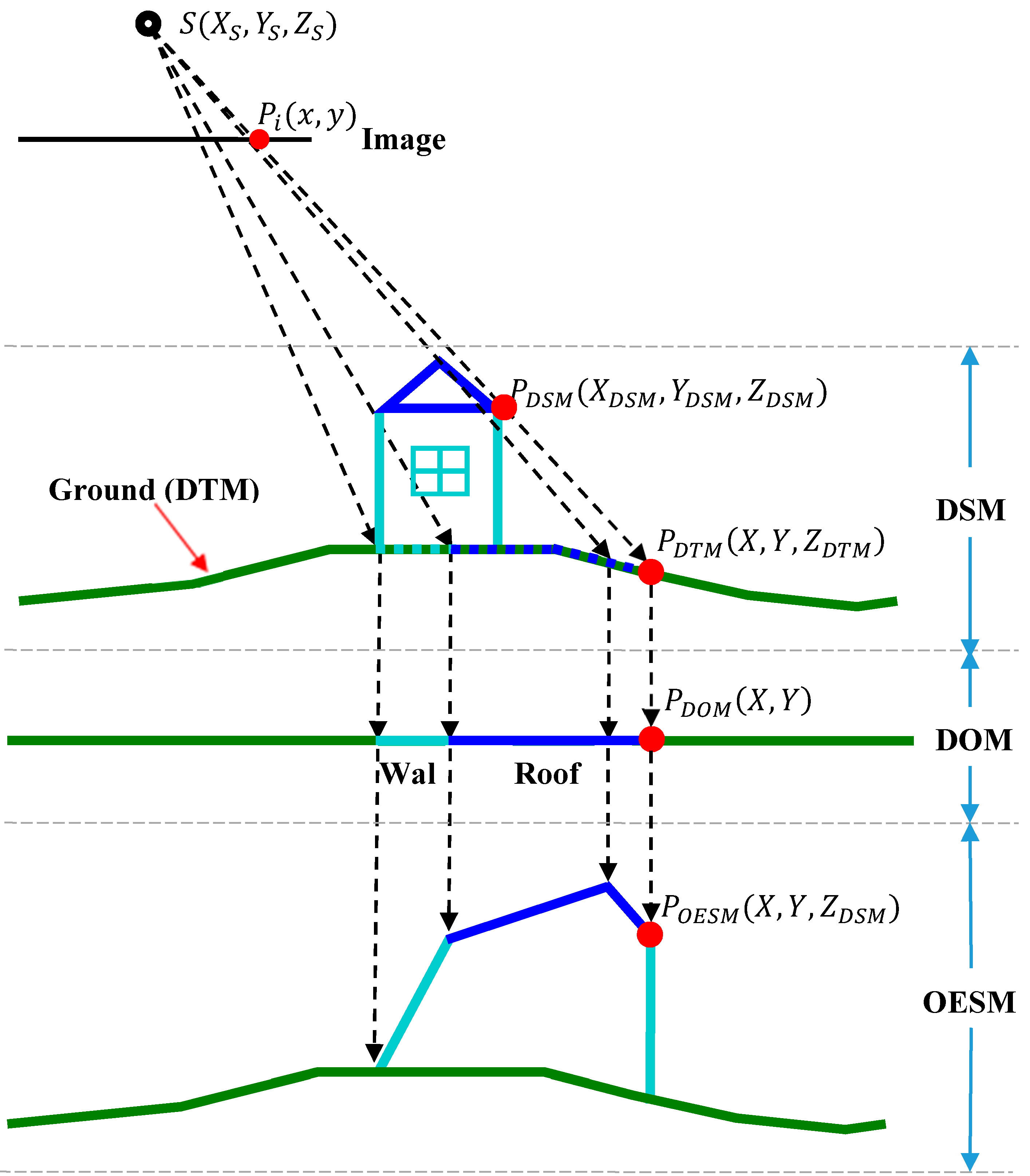
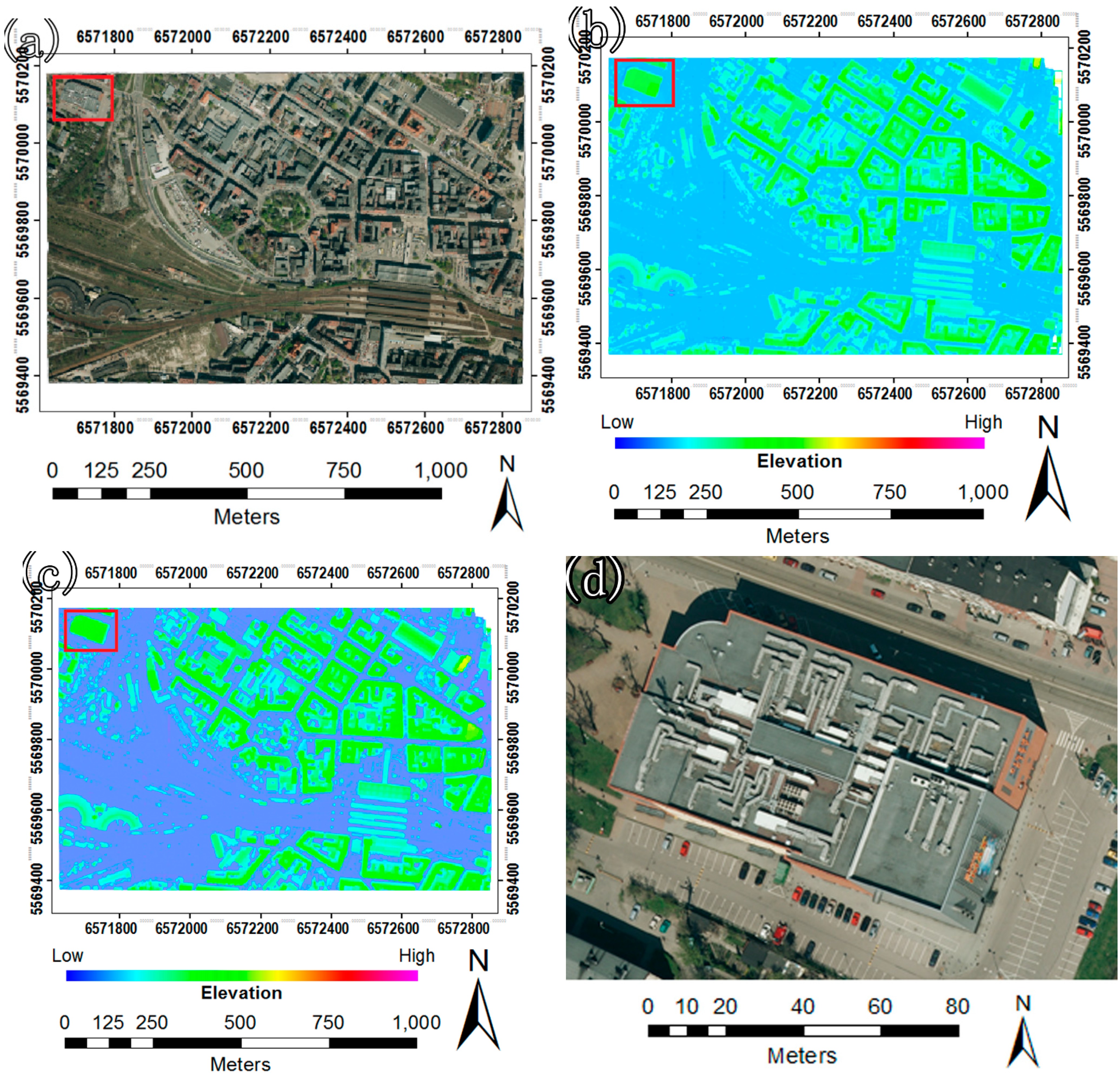
2.1. Orthoimage Elevation Synchronous Model

Rectification with a DTM for DOMs can only eliminate the effect of the perspective projection of the terrain, but relief displacement still exists with various ground objects, such as houses, bridges and trees. Although a DSM contains the elevation information of such objects, the elevation values are actually partly misplaced relative to the corresponding objects, because of relief displacement. To assign an accurate elevation value for every DOM unit, an OESM is derived and introduced. An OESM can reflect the actual elevation of each DOM unit. In an OESM, terrain elevations are from a DTM, whereas object elevations are from a DSM.

The OESM principle is shown in Figure 2. $P_{DSM}$ is the point on the DSM pertaining to a building point. After connecting the perspective center $S$ to $P_{DSM}$, the point on the DTM ($P_{DTM}$) and the corresponding point on the DOM ($P_{DOM}$) can be calculated through the intersection of $S{P}_{DSM}$ and DTM. By replacing the elevation of $P_{DTM}$ ($Z_{DTM}$) with the elevation of $P_{DSM}$ ($Z_{DSM}$), the coordinate of the corresponding point on the OESM ($P_{OESM}$) is obtained. For the terrain point of the DSM, the elevation of the intersection point is equivalent to the DTM, such that the elevation of the OESM is accordant with that of a DTM in this case. The figure shows that the OESM can reflect the actual elevation information of the DOM.

Figure 2. Geometric relationship of DSM, DTM, DOM, and the proposed OESM. $S$ is the perspective center; $P_i$, $P_{DSM}$, $P_{DTM}$ and $P_{DOM}$ are the corresponding points of the original image, DSM, DTM and DOM, respectively; and $P_{OESM}$ is the corresponding point of the proposed orthoimage elevation synchronous model (OESM).

Figure 2. Geometric relationship of DSM, DTM, DOM, and the proposed OESM. $S$ is the perspective center; $P_i$, $P_{DSM}$, $P_{DTM}$ and $P_{DOM}$ are the corresponding points of the original image, DSM, DTM and DOM, respectively; and $P_{OESM}$ is the corresponding point of the proposed orthoimage elevation synchronous model (OESM).

The solution for the intersection point ($P_{DTM}$) of $S{P}_{DSM}$ and DTM is described as follows: The geometric relationship of $S$ and an arbitrary object point can be represented as:

$${\left[X,Y,Z\right]}^T=[X_S,Y_S,Z_S]{ }^T+\mathrm{\lambda }·{\left[\delta X,\delta Y,\delta Z\right]}^T (\mathrm{\delta }Z\ne 0)$$

(1)

where $X$, $Y$ and $Z$ are the coordinates of the object point; $X_S$, $Y_S$ and $Z_S$ are the coordinates of the perspective center; ${[\text{δ}X,\text{δ}Y,\text{δ}Z]}^T$ is a unit vector along the ray connected by S and the object point; and $\text{λ}$ is the scaling coefficient.

For points $P_{DSM}$ and $P_{DTM}$ in Figure 2:

$$\{\begin{array}{c}\begin{array}{c}{\left[X_{DSM},Y_{DSM},Z_{DSM}\right]}^T=[X_S,Y_S,Z_S]{ }^T+{\text{λ}}_{DSM}\times {[\text{δ}X,\text{δ}Y,\text{δ}Z]}^T\end{array}\\ {\left[X,Y,Z_{DTM}\right]}^T=[X_S,Y_S,Z_S]{ }^T+{\text{λ}}_{DTM}\times {[\text{δ}X,\text{δ}Y,\text{δ}Z]}^T\end{array}$$

(2)

Given that ${\left[X_{DSM},Y_{DSM},Z_{DSM}\right]}^T$ and $[X_S,Y_S,Z_S]{ }^T$ are known, ${[\text{δ}X,\text{δ}Y,\text{δ}Z]}^T$ can be solved.

Thus, for a given $Z_{DTM}$, we can obtain:

$${\text{λ}}_{DTM}=(Z_{DTM}-Z_S)/\mathrm{\delta }Z$$

(3)

and then:

$${\left[X,Y\right]}^T=[X_S,Y_S]{ }^T+{\text{λ}}_{DTM}\times {[\text{δ}X,\text{δ}Y]}^T$$

(4)

The calculation of $Z_{DTM}$ is an iterative approximation process, the principle of which is described in Figure 3. First, $P_{DSM}$ is projected vertically onto a DTM to obtain an initial elevation value ($Z_0$), and then, the coordinates of $P_0(X_0,Y_0,Z_0)$ can be calculated according to Formulas (3) and (4). $P_0$ is also projected onto the DTM, and the elevation of $P_0^{\text{'}}$ ($Z_1$) can then be obtained. Again, $P_1(X_1,Y_1,Z_1)$ can be calculated according to Formula (3) and (4). Thus, the coordinates of the intersection point can be approximated as $P_{DTM}(X_n,Y_n,Z_n)$ when $\left|Z_n-Z_{n-1}\right|$ is small enough.

Figure 3. Iteration process of calculating the intersection point of $S{P}_{DSM}$ and a DTM.

Figure 3. Iteration process of calculating the intersection point of $S{P}_{DSM}$ and a DTM.

In fact, the iterative method adopted in our approach could be divergent or incorrect in some cases. According to Sheng’s research, the iteration will be convergent only if the terrain slope angle is smaller than the view elevation angle [31]. However, in aerial photogrammetry, the minimum view elevation angle always has a relatively large value (which is at least 55° in our experimental datasets); meanwhile, a steep slope is generally infrequent in urban areas. Therefore, the method will work properly in most cases. In actual processing, if the iteration times of a DSM point exceed a large number, then the point will be treated as an invalid point, and the elevations of the corresponding point in OESM will remain as the DTM elevation.

From the above discussion, the OESM generation procedure using a DSM and a DTM is as follows:

(1)

A blank OESM is created with the same range and grid size as those of the DTM.

(2)

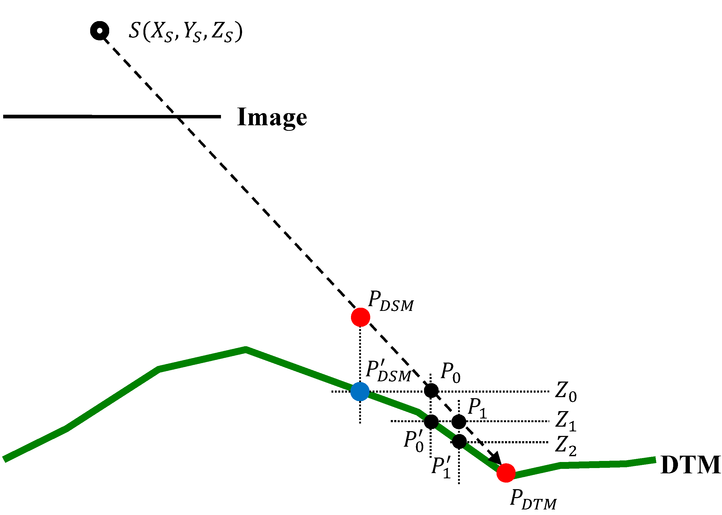
The coordinates for each point projected from the DSM to the DTM are calculated, and the elevation value of the projected point is replaced with that of the DSM point using the aforementioned method. The point with an updated elevation is then added to the created OESM. When two or more DSM points are projected onto the same grid in OESM, the principle of Z-buffer [32] is adopted to determine which points are occluded by others. The distances from the projection center to all of the points are calculated; the point with a minimum distance is considered visible, and its elevation will be assigned to the OESM grid, whereas other points are regarded as occluded.

(3)

After completing the projection for all DSM points, a Delaunay triangulated irregular network is constructed using all of the added grid points [33], and the complete OESM can be obtained through interpolation.

Figure 4 shows the overlying views between a DOM and the elevation contours of a DSM or OESM. To eliminate the terrain effect, both DSM and OESM are normalized by deducting the elevation value of the corresponding position in a DTM. Given that small displacement occurs when projecting DSM points onto OESM grids, a certain height error may be brought to the normalized OESM when deducting DTM elevation. However, the error would be limited in most cases, because terrain undulation is generally flat within a small area, especially in urban areas. Evidently, for a similar building, the elevation contours of a DSM accumulate around the building toft and cannot correctly reflect the elevation change in a DOM, whereas the OESM elevation contours accurately reflect the elevation change of walls and is thus appropriate for building edges. Hence, an OESM is obviously more suitable than a DSM for seamline selection apart from buildings.

2.2. Seamline Selection between Two DOMs

Given the existing rotation angle from the imaging altitude of the camera, the image file of a DOM always has some blank areas around the boundary. As shown in Figure 5, the effective area of the image should be extracted for mosaicking. In our research, the Moore–Neighbor tracing algorithm [34] is adopted to obtain the boundary pixels of the effective area, and simplification is performed on the basis of the Douglas–Peucker algorithm [35] to reduce the number of boundary points. A seamline is selected from the overlap between the effective areas of two images. Before selection, the two intersection points of the effective areas are determined as the start and end points, whereas the straight skeleton of the overlap is extracted as the initial seamline [36]. In our method, the final seamline selected should be as close as possible to the initial seamline, because the relief displacement of the ground object becomes great while approaching the image boundary, and the straight skeleton can be located in the middle part of the overlap with an arbitrary shape.

Figure 4. Overlying views between a DOM and the elevation contours of a DSM or OESM. (a–c) The DOM and the elevation renderings of the normalized DSM and OESM in the same area, respectively; (d) the image in the red rectangular area; and (e,f) the overlying views between a DOM and the elevation contours of a DSM or OESM in the red rectangular area, respectively.

Figure 4. Overlying views between a DOM and the elevation contours of a DSM or OESM. (a–c) The DOM and the elevation renderings of the normalized DSM and OESM in the same area, respectively; (d) the image in the red rectangular area; and (e,f) the overlying views between a DOM and the elevation contours of a DSM or OESM in the red rectangular area, respectively.

After determining the overlapping area of two DOMs, OESM data are used to generate an initial path network for seamline selection. First, with the use of existing DSM and DTM data, the OESM data of the two images are calculated. Second, the normalized OESM is obtained by deducting the DTM elevation in the same area. After normalization, OESM only maintains the height information above the terrain. The normalized OESM of the two images can then be added up and binarized using the following equation:

$$g\left(x,y\right)=\{\begin{array}{c}255, h_1\left(x,y\right)+h_2\left(x,y\right)>T_h\\ 0, otherwise\end{array}$$

(5)

where $h_1(x,y)$ and $h_2(x,y)$ are the height values of two normalized OESM data at the same point, $g(x,y)$ is the gray value of the corresponding point in the binary image and $T_h$ is the given height threshold determined by the height of the lowest object that needs to be avoided. In our approach, $T_h$ is set to 2.0 m. Figure 6a shows the binary image of the overlapping area in Figure 5 obtained through the above method.

The black region in the binary image indicates the area with a lower height than $T_h$. Most of the high ground objects can be avoided if the seamline is chosen from the black region. For the black region positioned between two white regions (such as road areas), extracting the middle line of the black region as the seamline is appropriate, because although the height at the edge of the white region is lower than $T_h$, this area can still be very close to $T_h$. Therefore, the Hilditch algorithm [37] is used to thin the black region and to obtain the middle lines for all of the black regions. Figure 6b shows the thinning result.

Figure 5. Determining the overlapping areas among DOMs and the extraction of the straight skeleton for the overlap. The red dashed line is the effective area of the top DOM. The green dashed line is the effective area of the bottom DOM. The white dotted line is the overlapping area between two DOMs. The white solid line is the extracted straight skeleton.

Figure 5. Determining the overlapping areas among DOMs and the extraction of the straight skeleton for the overlap. The red dashed line is the effective area of the top DOM. The green dashed line is the effective area of the bottom DOM. The white dotted line is the overlapping area between two DOMs. The white solid line is the extracted straight skeleton.

Figure 6. Binarization and thinning results for the OESM data of the overlapping areas in Figure 5. (a) Binary image of the overlapping area in Figure 5 in which the white region is the higher area and the black region is the lower area; (b) thinning result of the black region of (a).

Figure 6. Binarization and thinning results for the OESM data of the overlapping areas in Figure 5. (a) Binary image of the overlapping area in Figure 5 in which the white region is the higher area and the black region is the lower area; (b) thinning result of the black region of (a).

The above thinning result is the initial path network, from which the final seamline is extracted according to the following procedures:

(1)

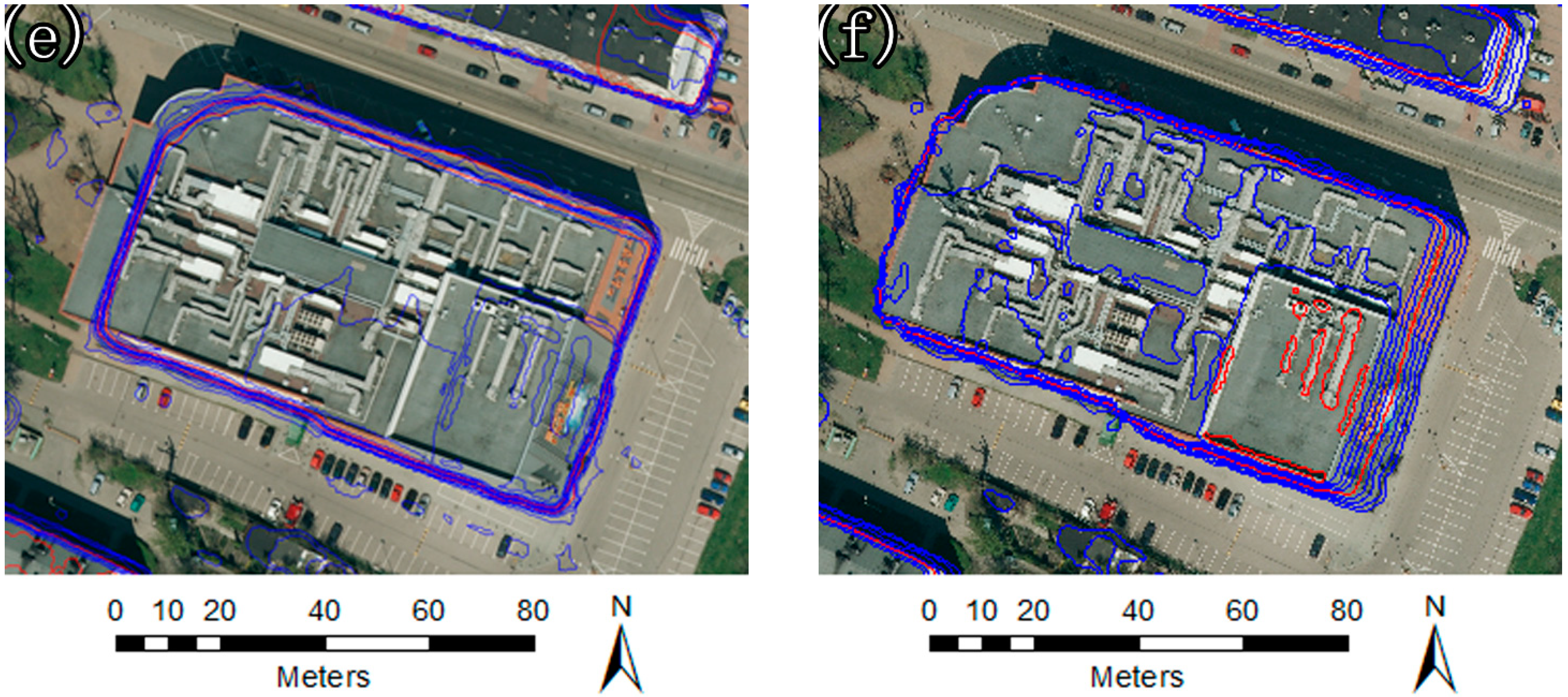
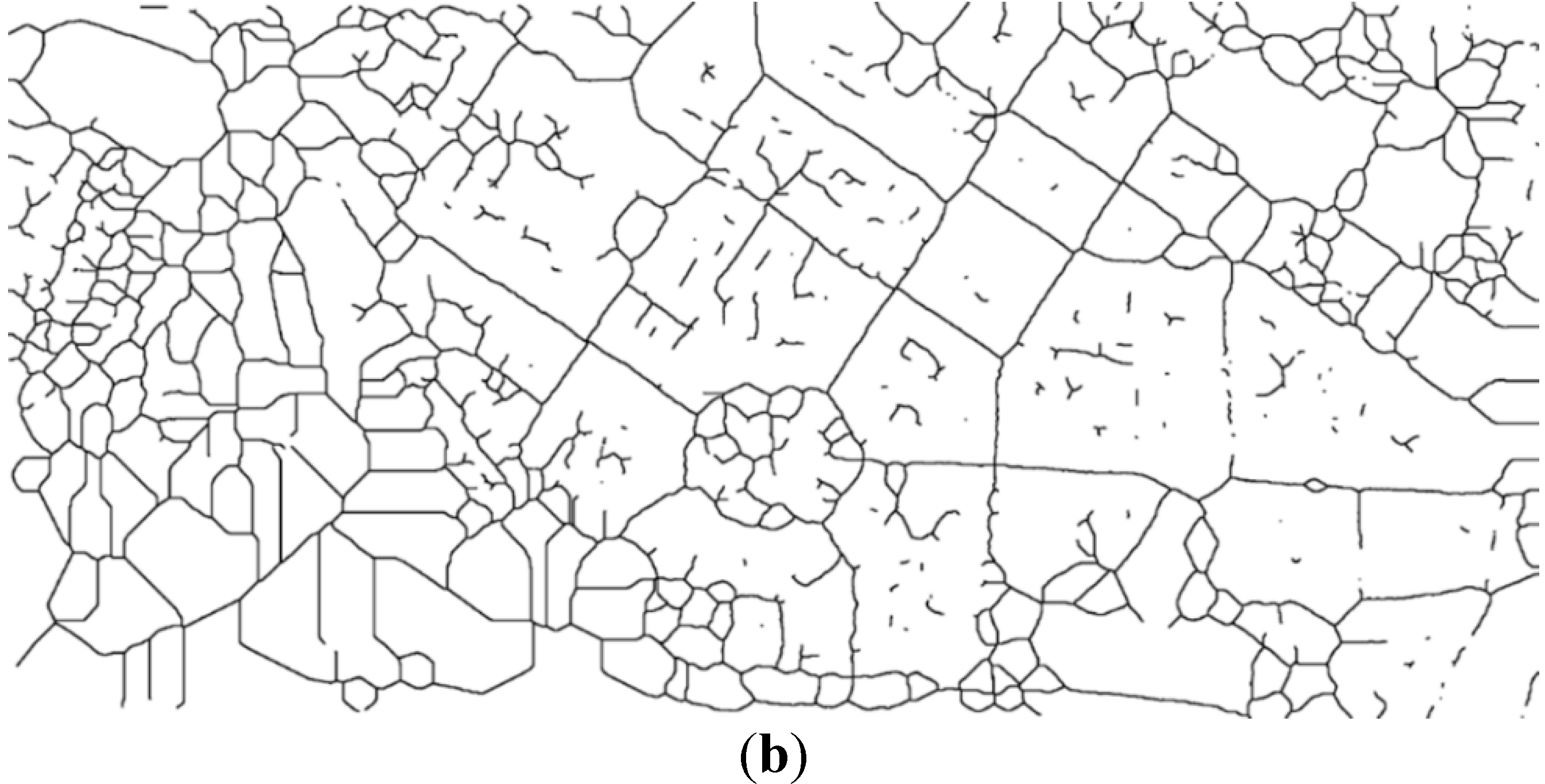
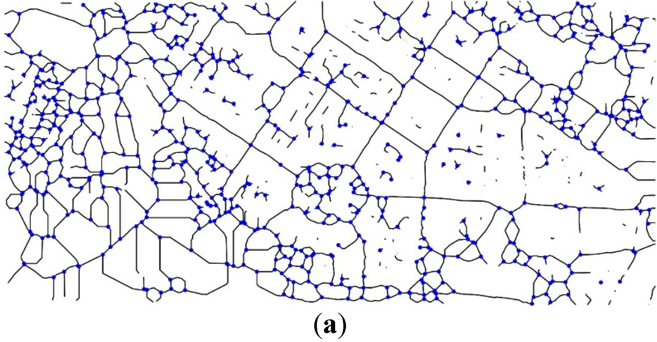
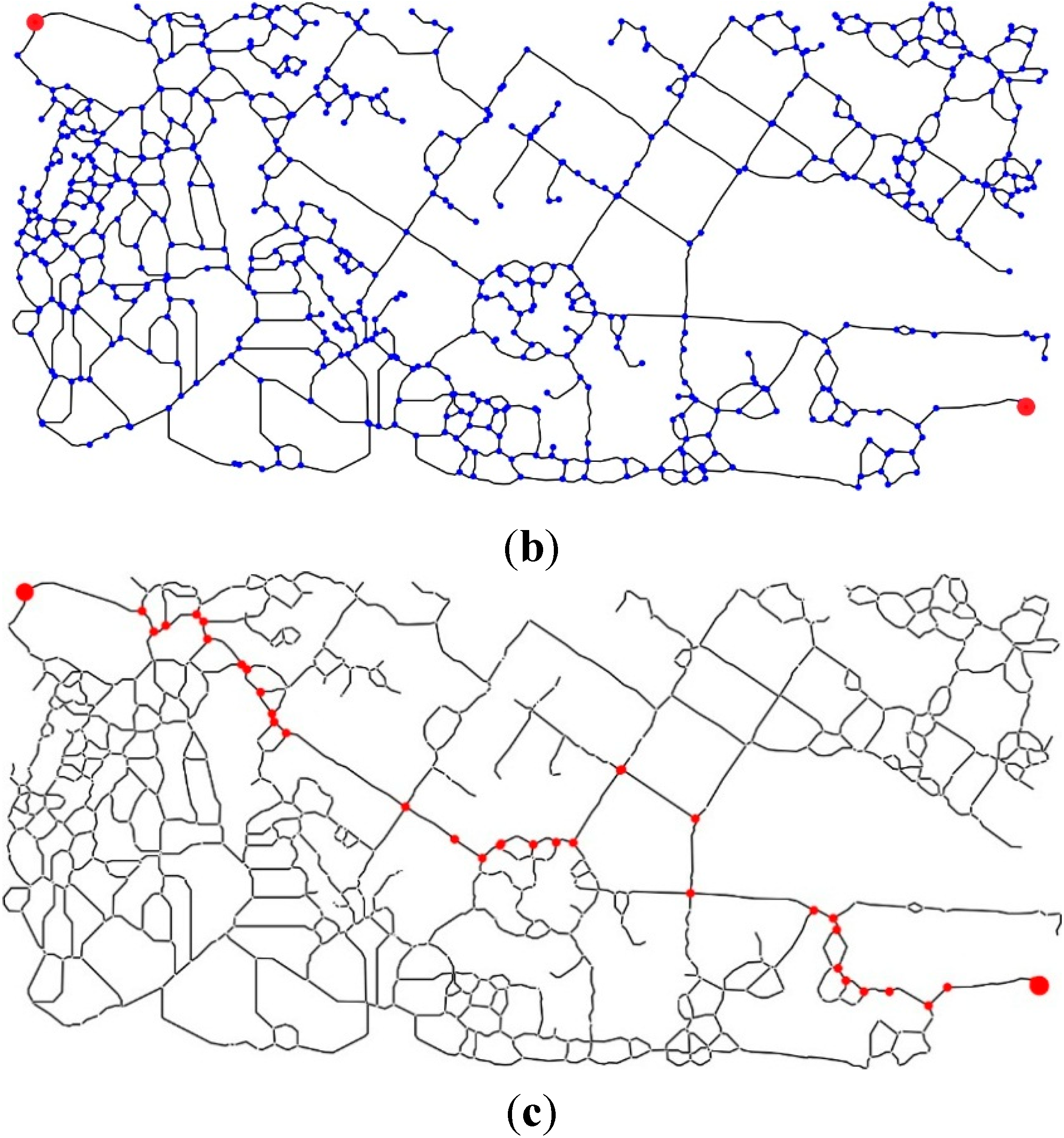
Candidate nodes and segments are determined from the network. First, intersection points with at least three paths crossing are selected as candidate nodes, as shown in the blue solid dots in Figure 7a. Next, the lines connected by two neighboring candidate nodes are considered as segments.

(2)

The useless nodes and segments are removed. First, the two candidate nodes nearest to the endpoints of the initial seamline (the skeleton) are chosen as the entrance and exit points, respectively (as shown in the red solid dots in Figure 7b). Subsequently, every candidate node is checked by assessing whether such a node can be connected to the entrance and exit through several segments. If the node is disconnected from the entrance or exit, this node is deleted. After removing all of the useless nodes, the segments that meet the condition that any endpoint is no longer a candidate node are also deleted. Figure 7b shows the path network without the redundant nodes and segments.

(3)

The least-cost path is determined as the seamline from the simplified network.

Figure 7. Procedures for obtaining the seamline from the initial path network. (a) Selection of the candidate nodes, where the blue solid dots represent the intersection points with at least three paths crossing; (b) the path network after removing the redundant nodes and segments, with the red solid dots representing the entrance and exit points; (c) the least-cost path determined on the basis of Dijkstra’s algorithm; the red solid dots represent the nodes of the determined path.

Figure 7. Procedures for obtaining the seamline from the initial path network. (a) Selection of the candidate nodes, where the blue solid dots represent the intersection points with at least three paths crossing; (b) the path network after removing the redundant nodes and segments, with the red solid dots representing the entrance and exit points; (c) the least-cost path determined on the basis of Dijkstra’s algorithm; the red solid dots represent the nodes of the determined path.

In our approach, the local cost between any two connected nodes is defined as:

$$Cost\left(i,j\right)=L\left(i,j\right)\times D(i,j)/W(i,j)$$

where $i$ and $j$ represent two neighboring and connected nodes. $Cost\left(i,j\right)$ is the cost value between $i$ and $j$. $L\left(i,j\right)$ is the path length (pixel numbers) in the network between $i$ and $j$. $D(i,j)$ is determined by calculating the vertical distance from $i$ and $j$ to the skeleton segments. Only if the perpendicular foot lies within the skeleton segment will the distance from the node to the segment be considered valid. As shown in Figure 8a, $i$ has two valid distances ($D_1$ and $D_2$), whereas $j$ has only one valid distance. The largest value of the valid distances will be assigned to $D(i,j)$. $D(i,j)$ represents the distance of the path from the initial seamline, which is proportional to the cost value. $W(i,j)$ is used to describe the pre-thinning width of the path segment. As shown in Figure 8b, $W(i,j)$ is obtained through the following method: (1) the middle point of the path is determined, and its pixel coordinates are obtained; (2) on the basis of morphological methods, the middle point is dilated using a circle element until the dilated and while regions intersect; and (3) the diameter of the dilated circle is extracted as $W(i,j)$. A great $W\left(i,j\right)$ means a small cost.

Based on the above defined cost function, the least-cost path can be obtained by using Dijkstra’s algorithm. Figure 7c shows the final determined seamline.

The EMPs of the two DOMs can be determined by updating the effective area with the seamline. Figure 9 shows the mosaicking result by filling the images according to the EMP. The result indicates that the selected seamline is located at low elevated places, and most high ground objects, such as buildings and tall trees, are successfully avoided.

Figure 8. Calculation methods for $D(i,j)$ and $W(i,j)$. (a) The red polyline is part of the skeleton. The blue polyline is a path segment, and the blue solid dots are nodes of the segment. (b) The white region is the higher area, and the black region is the lower area. The orange solid dot is the middle point of the path, and the light orange area is the dilated region of the middle point.

Figure 8. Calculation methods for $D(i,j)$ and $W(i,j)$. (a) The red polyline is part of the skeleton. The blue polyline is a path segment, and the blue solid dots are nodes of the segment. (b) The white region is the higher area, and the black region is the lower area. The orange solid dot is the middle point of the path, and the light orange area is the dilated region of the middle point.

Figure 9. Mosaic result of the two DOMs. The green lines show the determined effective mosaic polygons (EMPs) for the images. The yellow crosses and characters indicate the nadir points and file names of the images.

Figure 9. Mosaic result of the two DOMs. The green lines show the determined effective mosaic polygons (EMPs) for the images. The yellow crosses and characters indicate the nadir points and file names of the images.

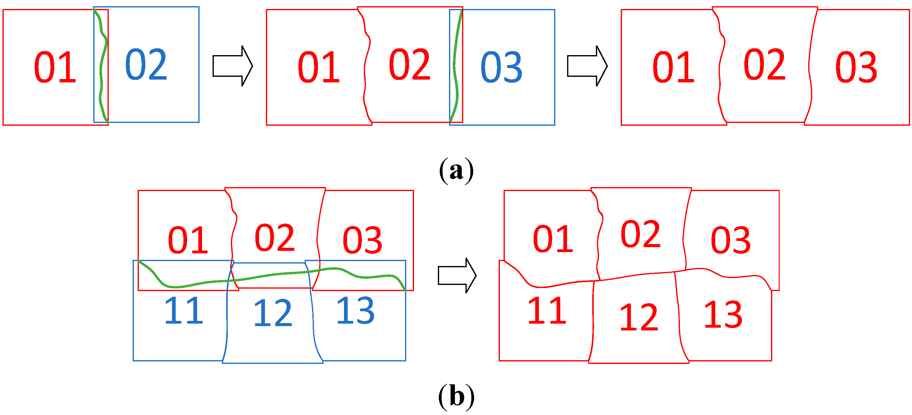
2.3. Construction of the Seamline Network

For DOM mosaicking applications in actual production, the input data always comprise a series of images captured in a large flight area, and the expected mosaicking result is composed of more than two images. To obtain a seamline network for multiple DOMs, the strip information recorded in flight is used in our approach. The steps of seamline network construction are as follows:

(1)

According to the flight order, the seamline between each of two adjacent DOMs in one flight strip is selected successively. When the seamline between the first image and the adjacent image is determined, the two images are treated as a mosaic. If another image exists in the same strip, a new seamline is determined between the mosaic and the newly-added image, and a new mosaic with three images is obtained. Therefore, all of the images along the same strip are processed, and the EMPs for these images are determined.

(2)

With the use of the same method, the seamline between each two adjacent strips is selected according to the strip order. Every time a seamline between two strips is determined, the EMPs of all of the preprocessed images are updated with the newly-added seamline.

Figure 10 shows an example of the seamline network construction for two strips, where every strip contains three images.

Figure 10. Construction of a seamline network. (a) Construction process for images in one strip; (b) construction process for adjacent strips. The red part represents the determined EMPs. The blue part represents the newly-added image. The green line represents the newly-selected seamline. 01, 02 and 03 represent the three images in the first strip, while 11, 12 and 13 represent the three images in the second strip.

Figure 10. Construction of a seamline network. (a) Construction process for images in one strip; (b) construction process for adjacent strips. The red part represents the determined EMPs. The blue part represents the newly-added image. The green line represents the newly-selected seamline. 01, 02 and 03 represent the three images in the first strip, while 11, 12 and 13 represent the three images in the second strip.

3. Experiments and Results

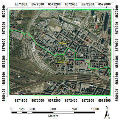
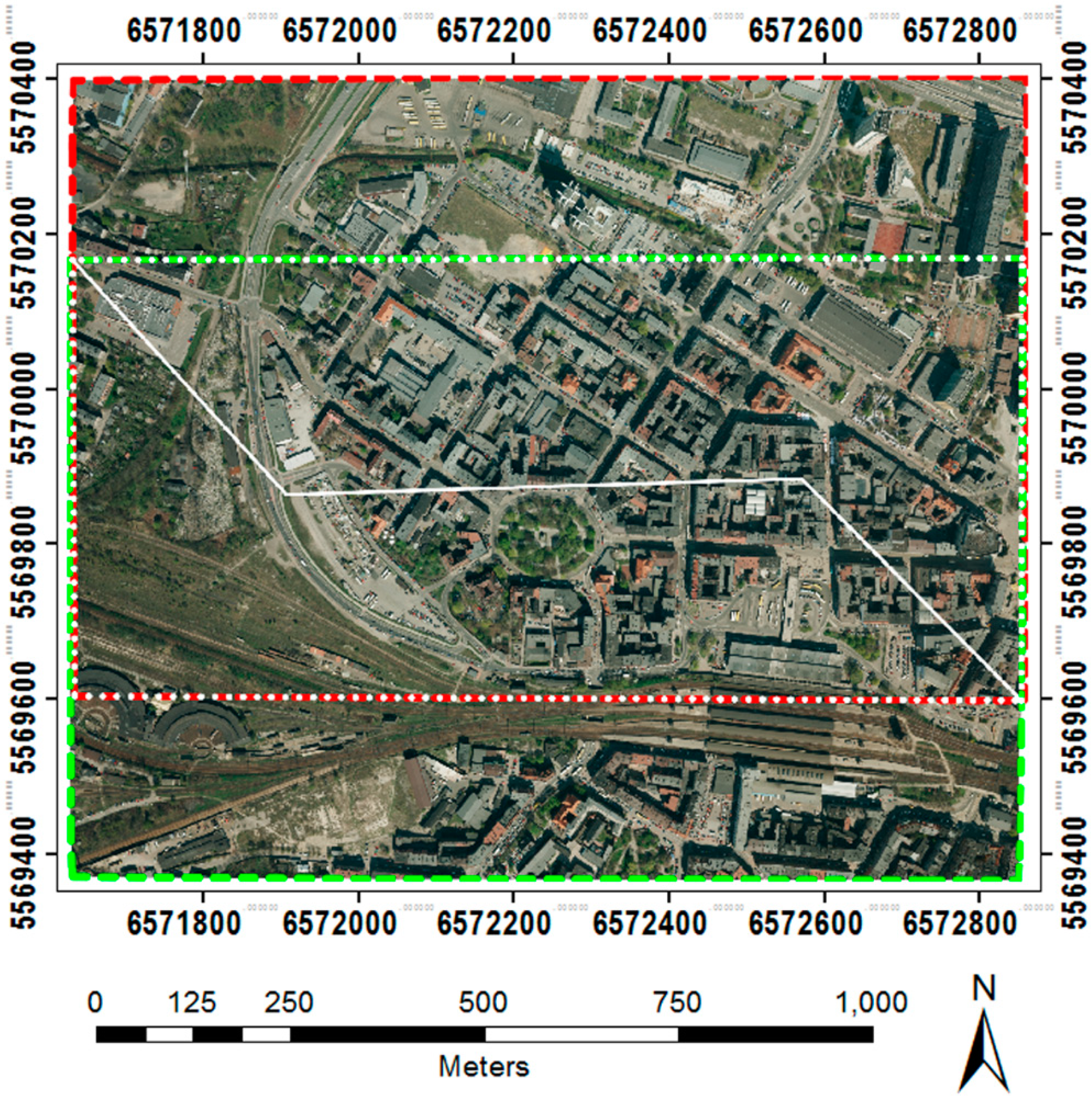
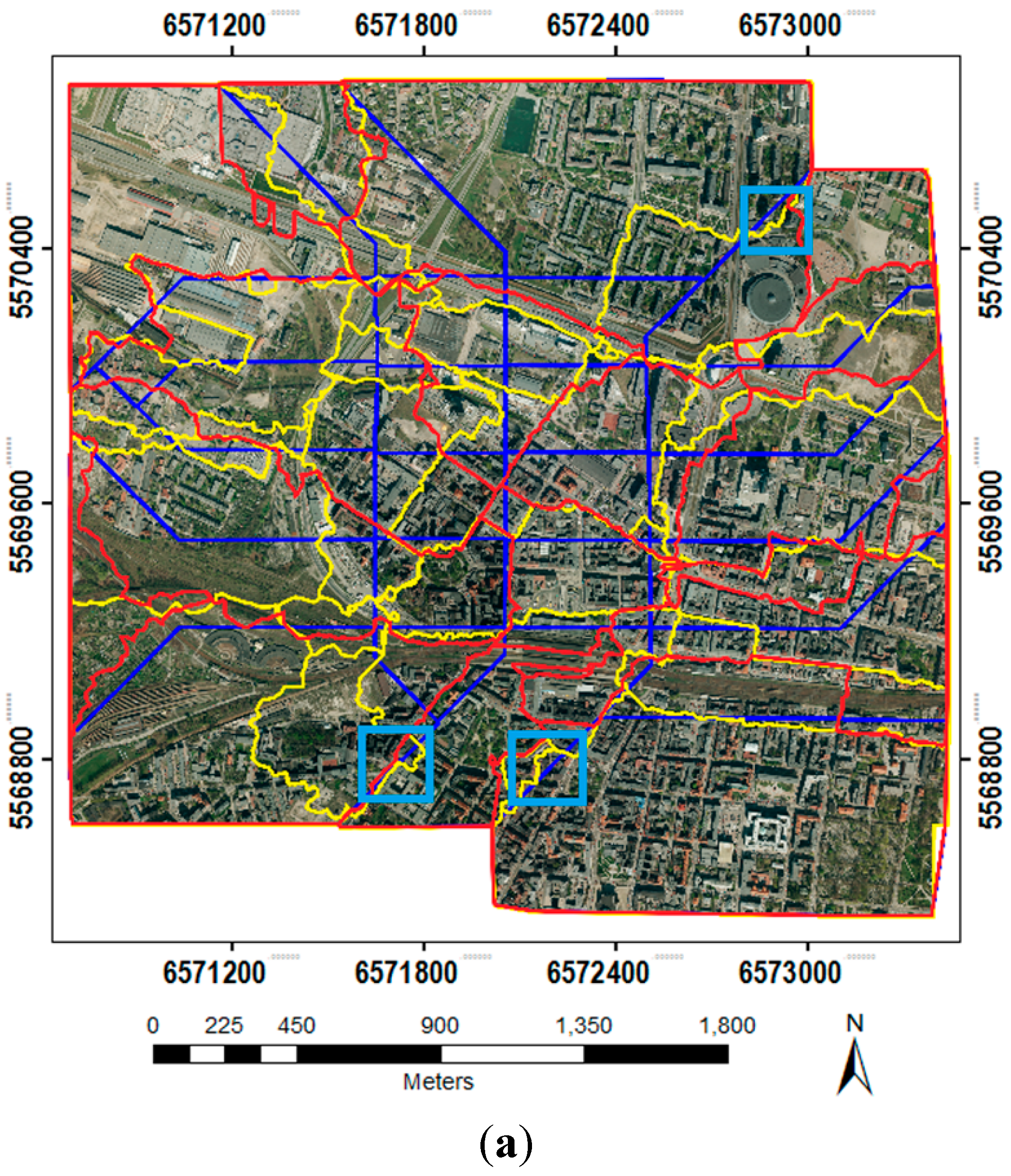
3.1. Data Preparation

Three datasets from different areas were used in the experiments to evaluate the performance of the proposed approach. The first dataset contained 24 images with a size of 17,310 × 11,310 pixels, and the test area was in Katowice, Poland, with medium-sized buildings. The second dataset contained 14 images with a size of 7680 × 13,824 pixels, and the test area was in Vaihingen, Germany, with small-sized buildings. The third dataset contained 56 images with a size of 11,500 × 7500 pixels, and the test area was in San Francisco, USA, with numerous densely-distributed buildings. The details of the experimental datasets are shown in Table 1.

Table 1. Overview of test datasets.

Dataset ID	Location	Camera	Focal Length	Flying Height	Forward Overlap	Side Lap	Resolution	Spectral Bands
1	Katowice	UltraCam X	100.5 mm	1200 m	70%	70%	8 cm	R-G-B
2	Vaihingen	DMC	120 mm	900 m	60%	60%	8 cm	IR-R-G
3	San Francisco	UltraCam D	105.2 mm	1800 m	60%	30%	15 cm	R-G-B

Table 1. Overview of test datasets.

Dataset ID	Location	Camera	Focal Length	Flying Height	Forward Overlap	Side Lap	Resolution	Spectral Bands
1	Katowice	UltraCam X	100.5 mm	1200 m	70%	70%	8 cm	R-G-B
2	Vaihingen	DMC	120 mm	900 m	60%	60%	8 cm	IR-R-G
3	San Francisco	UltraCam D	105.2 mm	1800 m	60%	30%	15 cm	R-G-B

Before mosaicking, all images were processed through image dodging and color balancing to minimize illustration differences. Aerial triangulation and bundle block adjustment were performed using ground control points to obtain the exterior orientation parameters of both datasets. To obtain a DSM, semi-global matching [38] was performed between the overlapping images in each strip. After generating and combining the DSM of the entire area, a filtering algorithm based on adaptive triangulated irregular network models [39] was adopted to obtain the ground points from the DSM. The DTM was generated by interpolating the ground points into a regular grid. To ensure the accuracy of the DTM, some manual intervention was required. With the resulting DSM and DTM, the OESM can be computed according to the method in Section 2.1.

All of the images were orthorectified to the 1984 World Geodetic System using the DTM, and the ground sampling distances of the DOMs in the datasets were 0.1, 0.1 and 0.2 m. With the use of the abovementioned OESM data, the seamline network was generated, and a seamless image mosaic was achieved for each dataset.

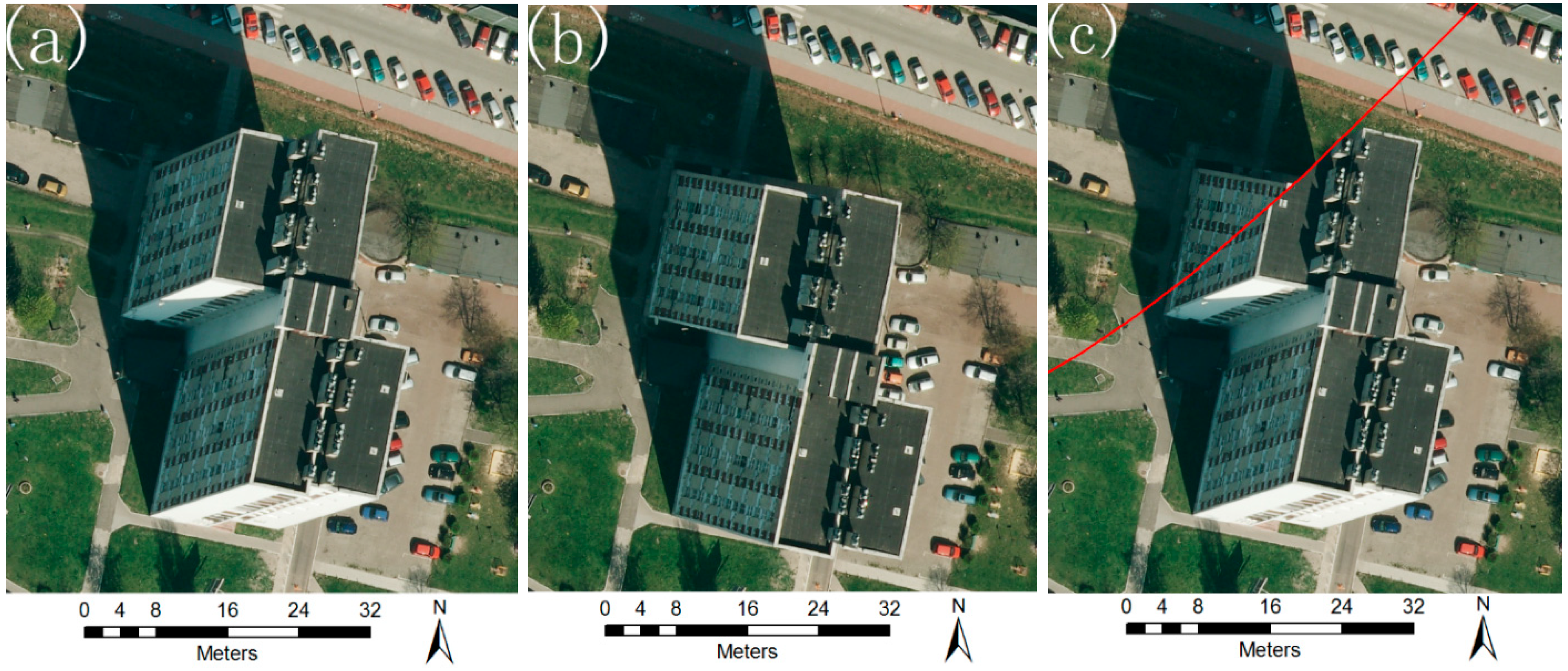
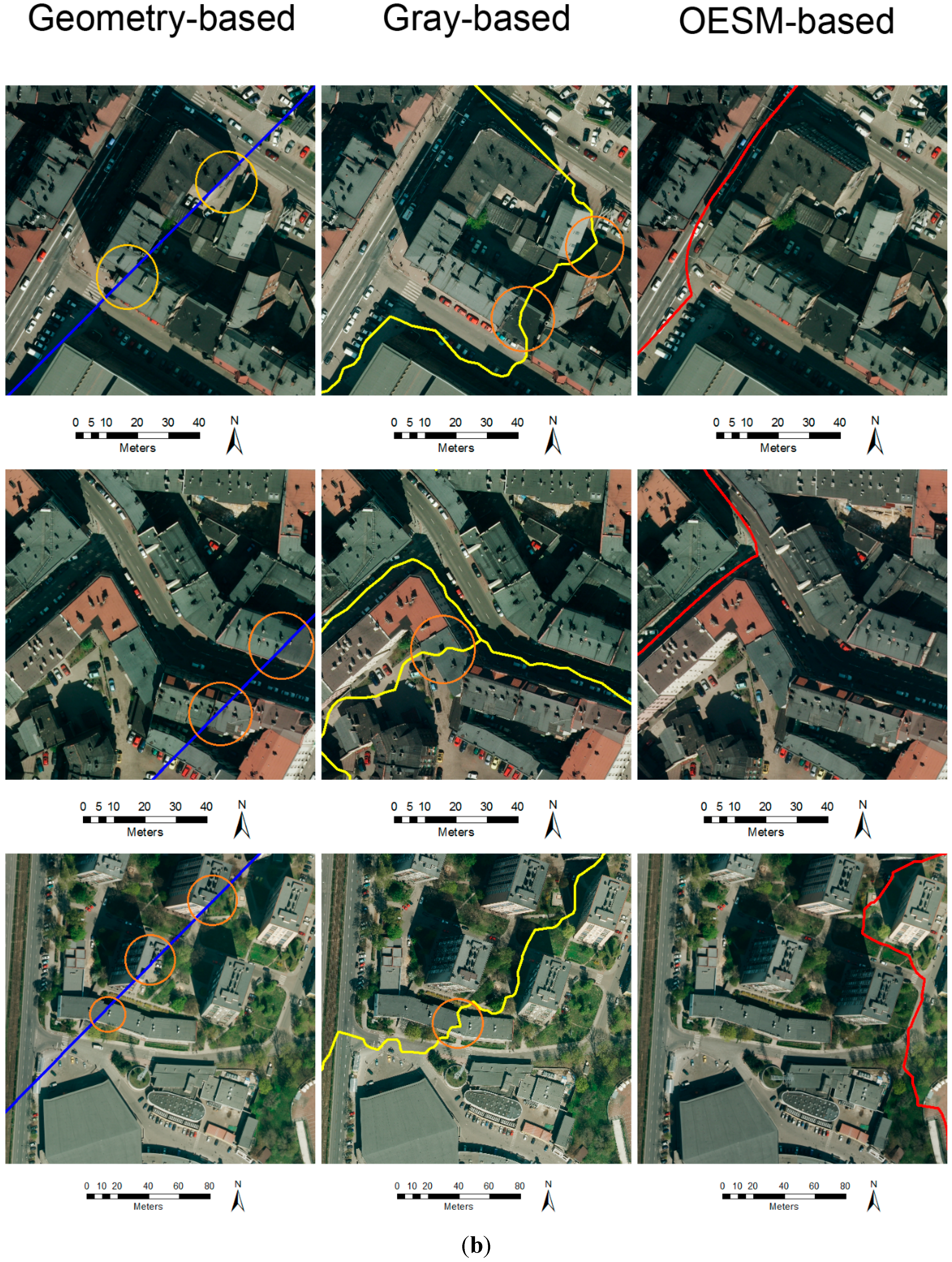
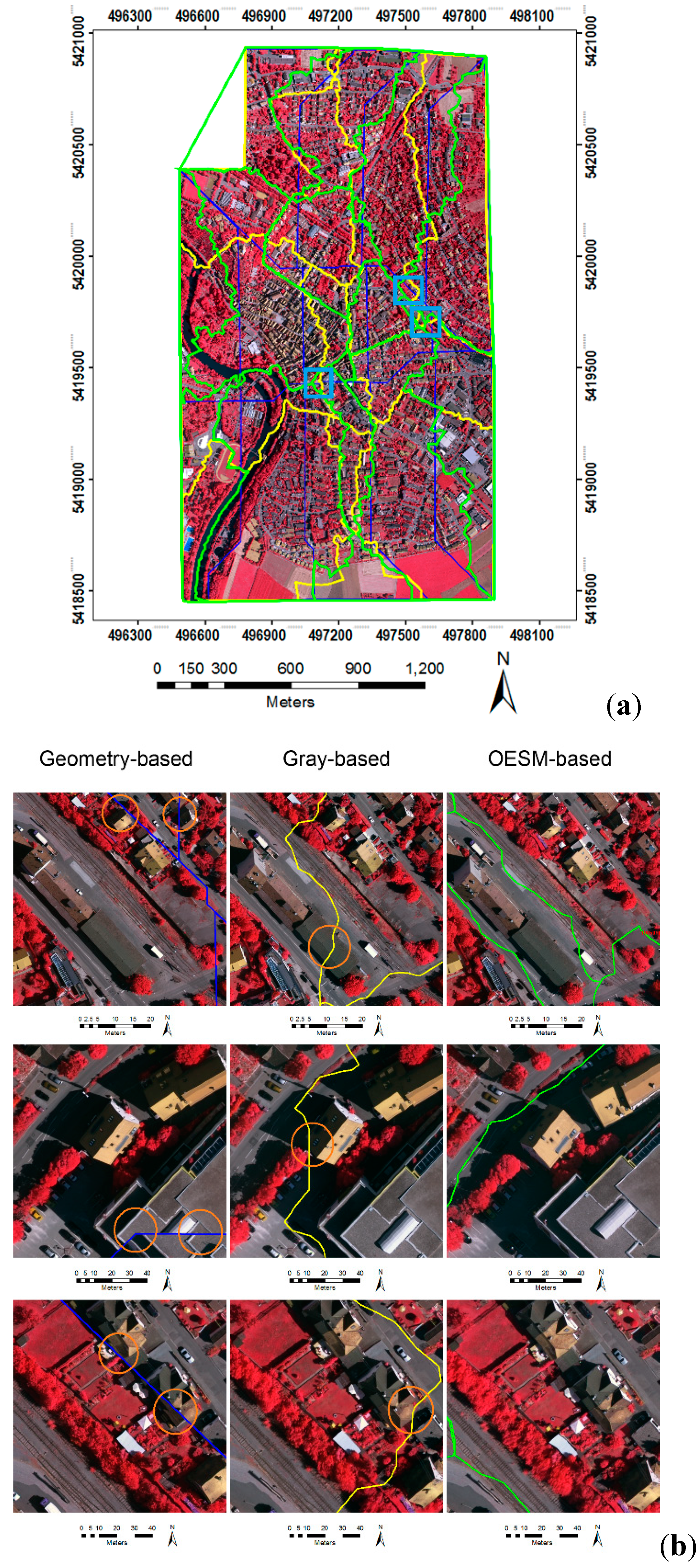
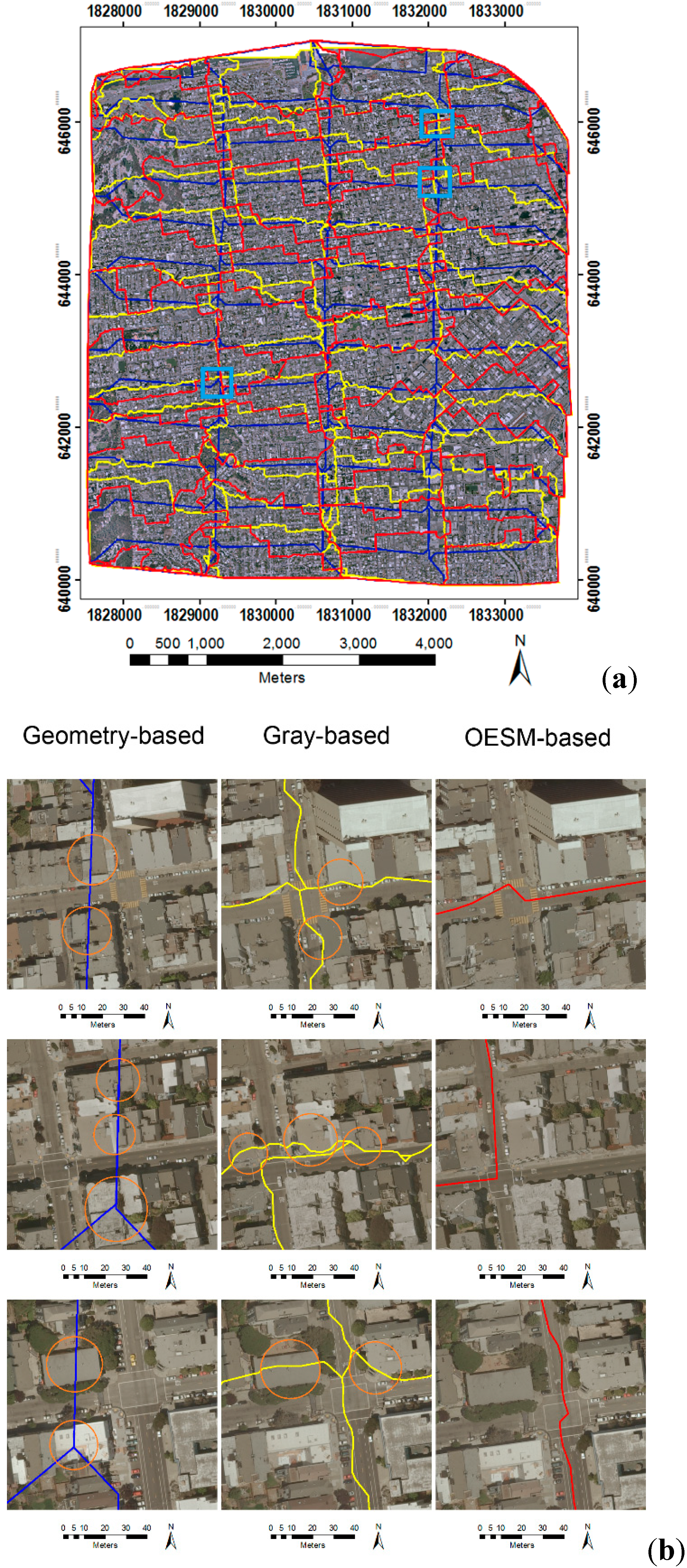
3.2. Evaluation and Comparison

All of the aforementioned algorithms were implemented using the C++ language. The Computational Geometry Algorithms Library was used to extract the straight skeleton in the overlapping area. A portable computer with a 64-bit Windows 7 operating system, a quad-core Intel Core i5-2520M CPU, 2.5 GHz and 4 GB memory was utilized for the experiments.

Given that the positioning accuracy of the DOMs in the same dataset was consistent, most visual discontinuities were caused by the seamlines passing through obvious objects (such as buildings). Therefore, similar to the evaluation method in other relevant studies [25,29], the mosaic results were evaluated by manually checking the number of times that seamlines passed through obvious objects. The difference was that when several grouped objects were crossed by a single seamline, such a seamline was only considered to pass through the objects once, because the visual discontinuity that occurred in such cases only resulted in one instance of manual editing in actual production.

Comparative experiments were conducted with three different methods. To evaluate the performances of these methods fairly, all of the methods were tested in a single thread, and only the processing time for the seamline network generation (not including the times of image filling and feathering) was recorded for comparison. The three methods were:

(1)

Without any optimization, the straight skeleton of the overlapping area was directly used as the seamline. In actual production, this method (or a similar method) is often used to generate an initial seamline network. Afterwards, manual editing is adopted on this basis.

(2)

Based on the image gray information, the seamline in the overlapping areas with minimal gray difference was selected. OrthoVista is one of the most powerful gray-based image mosaicking software; thus, the mosaicking function of the OrthoVista software [40] was adopted for comparison.

(3)

The proposed OESM method.

We refer to these methods as geometry-based, gray-based and OESM-based.

The mosaic results of the three datasets are shown in Figure 11, Figure 12 and Figure 13. According to the results, compared with the other two methods, the seamlines from the OESM-based method were more reasonable and successfully avoided intersecting most of the obvious objects. As shown in Table 2, in the OESM-based method, the obvious objects were intersected 9, 15 and 80 times. These values were evidently less than those of other methods. The processing time of the geometry-based method was significantly less than that of the other methods at the cost of seamline optimization. Comparing the almost similar seamline optimization performances, the OESM-based method was more efficient than the gray-based method.

Figure 11. Mosaic results of the three methods for Dataset 1. (a) Overview of the mosaicked images. The blue lines are the seamlines constructed through the geometry-based method; the yellow lines are the seamlines constructed through the gray-based method; and the red lines are the seamlines constructed through the OESM-based method. (b) Detailed seamlines in the cyan rectangular areas of (a) selected through the three methods. The orange circle marks the visual continuities from the seamlines.

Figure 11. Mosaic results of the three methods for Dataset 1. (a) Overview of the mosaicked images. The blue lines are the seamlines constructed through the geometry-based method; the yellow lines are the seamlines constructed through the gray-based method; and the red lines are the seamlines constructed through the OESM-based method. (b) Detailed seamlines in the cyan rectangular areas of (a) selected through the three methods. The orange circle marks the visual continuities from the seamlines.

Figure 12. Mosaic results of the three methods for Dataset 2. (a) Overview of the mosaicked images. The blue lines are the seamlines constructed through the geometry-based method; the yellow lines are the seamlines constructed through the gray-based method; and the green lines are the seamlines constructed through the OESM-based method. (b) Detailed seamlines in the cyan rectangular areas of (a) selected through the three methods. The orange circle marks the visual continuities from the seamlines.

Figure 12. Mosaic results of the three methods for Dataset 2. (a) Overview of the mosaicked images. The blue lines are the seamlines constructed through the geometry-based method; the yellow lines are the seamlines constructed through the gray-based method; and the green lines are the seamlines constructed through the OESM-based method. (b) Detailed seamlines in the cyan rectangular areas of (a) selected through the three methods. The orange circle marks the visual continuities from the seamlines.

Figure 13. Mosaic results of the three methods for Dataset 3. (a) Overview of the mosaicked images. The blue lines are the seamlines constructed through the geometry-based method; the yellow lines are the seamlines constructed through the gray-based method; and the red lines are the seamlines constructed through the OESM-based method. (b) Detailed seamlines in the cyan rectangular areas of (a) selected through the three methods. The orange circle marks the visual continuities from the seamlines.

Figure 13. Mosaic results of the three methods for Dataset 3. (a) Overview of the mosaicked images. The blue lines are the seamlines constructed through the geometry-based method; the yellow lines are the seamlines constructed through the gray-based method; and the red lines are the seamlines constructed through the OESM-based method. (b) Detailed seamlines in the cyan rectangular areas of (a) selected through the three methods. The orange circle marks the visual continuities from the seamlines.

Table 2. Comparison of the results of the different methods.

Method	Number of Times the Seamlines Pass through Obvious Objects			Processing Time (s)
	Dataset 1	Dataset 2	Dataset 3	Dataset 1	Dataset 2	Dataset 3
Geometry-based	236	193	Over 1500	47	20	80
Gray-based	26	24	325	2618	774	1718
OESM-based	9	15	80	1186	489	1375

Table 2. Comparison of the results of the different methods.

Method	Number of Times the Seamlines Pass through Obvious Objects			Processing Time (s)
	Dataset 1	Dataset 2	Dataset 3	Dataset 1	Dataset 2	Dataset 3
Geometry-based	236	193	Over 1500	47	20	80
Gray-based	26	24	325	2618	774	1718
OESM-based	9	15	80	1186	489	1375

The proposed method generally constructed the seamline network without passing through most of the obvious objects, and the obtained mosaic exhibited minimal visual discontinuity areas. As opposed to the comparative methods, the performance and efficiency of the proposed method more suitably met the requirements of actual production.

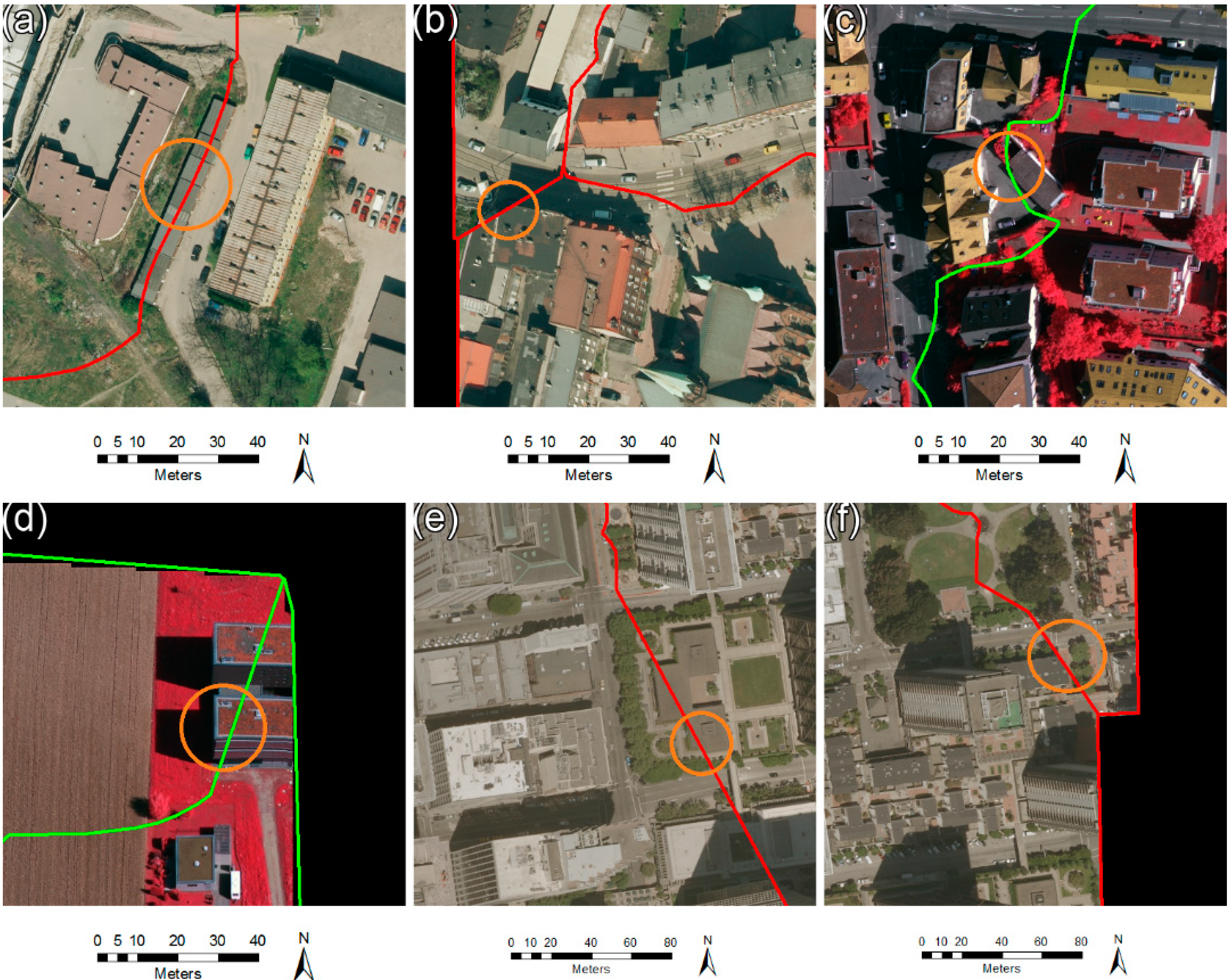
4. Discussion

An automatic seamline selection method using DSM data is proposed and applied to urban orthophoto mosaicking. The main feature of the proposed method is the use of an OESM calculated through DSM and DTM, instead of the direct use of a DSM, for seamless mosaicking. The elevation of the OESM, which is completely synchronous with that of DOMs, is applied as a guide for seamline selection. The results demonstrate the reliability and efficiency of the proposed method.

4.1. Seamline Selection Strategy

In related studies, most seamline optimization methods are developed on the basis of the analysis of the gray difference between overlapping images [12,20,25]. The main principle of these kinds of methods is selecting the path with minimal gray differences in the overlapped area as the seamline to meet the requirements of human vision. However, determining the seamline position on the basis of gray analysis may still cause the seamline to pass through obvious objects, because of the randomness and uncertainty of gray distribution in an image. For example, for a building with a roof that lacks texture in the overlapped area, a path with very low gray differences could be still found through the roof regardless of whether certain visual discontinuity results from relief displacement. In contrast to these methods, the proposed method selects seamlines on the basis of the elevation of objects, which is more reliable than basing on the gray analysis of images. By knowing the accurate elevation, most objects with elevations that exceed the designated threshold can be theoretically avoided by the seamlines generated through our method.

A comparison of the path searching strategies indicates that the main difference between our method and other methods (such as Chon et al.’s method [19] and Pan et al.’s method [25]) is that we search for the path from the connected path network instead of searching pixel-by-pixel. The advantage of this approach is evident, because the path network consists of thinning segments extracted from the black region, whereas most of the segments are located in the middle of the road. Compared with those selected by a pixel-based searching strategy, the seamlines selected by our method will be more regular. More importantly, we can infer that the efficiency of our method will be obviously better than those of other methods.

Wan et al. [24,27] and Ma et al. [29] indicate that better results can be obtained by using external data in seamline selection. However, precise vector road data are required in the method of Wan et al. [24,27]. Such data are hardly available in actual production. In addition, the research of Ma et al. [29] is challenged by unstable LiDAR data sources. Moreover, a DSM elevation is directly applied to detect obstacles without considering the influence of the relief displacement of objects, which cannot completely enable the seamline to avoid passing through objects theoretically. By contrast, the DSM data used in our approach are generated from dense matching stereo images. Given that stereo matching is significant in common photogrammetry workflows, a DSM can be obtained from a more stable source. Furthermore, an OESM calculated via DSM and DTM can reflect the elevation of objects on DOMs accurately. Theoretically, generating a seamline based on OESM is more rigorous than basing directly on a DSM.

In a standard production workflow, our method is practical in mosaicking applications for high-resolution urban images. Nevertheless, the proposed method also has limitations. In most cases, a seamline that can be selected from the generated path network always exists. However, on a few extremely rare occasions, no path can be searched from the path network. A typical situation is that a huge building with a minimum height higher than $T_h$ completely blocks the path between the entrance and exit points. In this case, the proposed approach will fail.

Moreover, using the proposed method for seamline selection in mosaicking applications with low-resolution images (such as medium-resolution satellite images) is unnecessary, because the influence of relief displacement in this resolution level is almost negligible. Meanwhile, fast mosaicking for initially obtained aerial images is required in some applications [41]. Given that the images for mosaicking are not orthorectified under this circumstance, the proposed method is likewise inapplicable to this case.

4.2. Accuracies, Errors and Uncertainties

In the test data, DOMs are rectified with orientation parameters after aerial triangulation and bundle block adjustment. Therefore, the positioning accuracy of DOMs is consistent. In many related studies, seamline quality is not generally evaluated through accuracy assessment. The quantitative index applied in this study is the number of times that seamlines pass through obvious objects. The results indicate that the number of times that seamlines pass through obvious objects is evidently less when using our method than when using other methods.

OESM with higher resolution may provide better precision for seamline selection. In our approach, the resolution of OESM is consistent with DTM, which is usually five- or 10-times the DOM resolution during the conventional production in aerial photogrammetry. However, our method uses the Hilditch algorithm to obtain the middle lines for all black regions after binarization. This process reduces the position error caused by relatively low OESM accuracy. If we try to create an OESM having the same resolution as DOM, the size of OESM will be 25- or 100-times the current size. Consequently, the time consumed by OESM generation will significantly increase, and the efficiency of the proposed approach could be significantly affected.

Figure 14 illustrates some situations in which the seamline generated by the proposed method passes through obvious objects. Two main situations are derived. First is when very low objects appear, which is mainly affected by the threshold value $T_h$ in Section 2.2. Regardless of whether the objects with elevations below $T_h$ can be passed through, the relief displacement of these objects is relatively small, which causes minimal visual influence. Second is when objects are located near the overlapping area boundary. In fact, visual discontinuities only exist beside the boundary of the entire survey area, because if discontinuities appear in the overlap of images along the same strip, they can mostly be eliminated through mosaicking between adjacent strips. The remaining discontinuities are difficult to eliminate. Given that the entrance and exit of a seamline must be located in the boundary, the seamline almost inevitably passes through these objects when such objects appear beside the entrance or exit. The experimental results confirm the analysis above, which shows that the objects near the boundary passed through the seamlines generated through our method, which is the same case as that of the seamlines generated by the other two methods.

Figure 14. Visual discontinuities (marked by the orange circles) caused by the seamlines of the OESM-based method. (a) The low elevated objects that are passed through in Dataset 1; (b) the objects near the boundaries that are passed through in Dataset 1; (c) the low elevated objects that are passed through in Dataset 2; (d) the objects near the boundaries that are passed through in Dataset 2; (e) the low elevated objects that are passed through in Dataset 3; (f) the objects near the boundaries that are passed through in Dataset 3.

Figure 14. Visual discontinuities (marked by the orange circles) caused by the seamlines of the OESM-based method. (a) The low elevated objects that are passed through in Dataset 1; (b) the objects near the boundaries that are passed through in Dataset 1; (c) the low elevated objects that are passed through in Dataset 2; (d) the objects near the boundaries that are passed through in Dataset 2; (e) the low elevated objects that are passed through in Dataset 3; (f) the objects near the boundaries that are passed through in Dataset 3.

In the proposed method, the most important factor affecting the quality of seamlines is the quality of DSM and DTM. Seamline selection is directly affected by the errors in the OESM. These faults are caused by the errors in DSM and DTM. However, the influence of the precision of DSM and DTM on the seamline network remains uncertain in this study. Furthermore, the three variables used in the cost function are not weighted. Variables with different weights may also influence the result. This case is not analyzed thoroughly in our approach.

5. Conclusions

A new method for automatic seamline network generation using digital surface model (DSM) data was proposed. Unlike traditional methods of selecting seamlines on the basis of gray information while relying on external data with unstable resources, seamlines are intelligently selected by applying DSM data obtained by stereo matching. One of the contributions of this study is the introduction of the new concept of the orthoimage elevation synchronous model (OESM), which accurately reflects the elevation value of every digital orthophoto map (DOM) unit by recovering the geometrical relationship among the DSM, digital terrain model and DOM.

An initial path network was generated for OESM data through binarization and thinning in the overlapping area of two images. With the cost function constructed through measurements, including the length, original path width and the distance from the path node to the straight skeleton, the least-cost path was determined using Dijkstra’s algorithm. Thereafter, by applying the selection method between two images to multiple images in a larger area, the seamline network was generated according to the strip information.

The experiments for three different datasets demonstrated that the numbers of times that the seamline network generated through an OESM passed through obvious objects were 9, 15 and 80, which were evidently less than the cases of seamlines generated by the geometry-based and OrthoVista methods. Under the same test conditions, the efficiency of the proposed method was also better than that of the OrthoVista method, given that the amounts of time consumed for the three datasets were 1186, 489 and 1375 s. In conclusion, the practicality and efficiency of our method can fully meet the application demands in actual production.

However, some further improvements are required. Numerous other path searching algorithms, aside from Dijkstra’s algorithm applied in this study, may yield better results in subsequent research. In addition, multiple overlaps (more than two images in the overlapped area) are not considered in the seamline selection of our approach currently. Hence, the optimal seamline generation based on multiple images will be considered in future studies.

References

- Helmer, E.H.; Ruefenacht, B. Cloud-free satellite image mosaics with regression trees and histogram matching. Photogramm. Eng. Remote Sens. 2005, 71, 1079–1089. [Google Scholar] [CrossRef]
- Soille, P. Morphological image compositing. IEEE Trans. Pattern Anal. Mach. Intell. 2006, 28, 673–683. [Google Scholar] [CrossRef] [PubMed]
- Yang, Y.; Gao, Y.; Li, H.; Han, Y. An algorithm for remote sensing image mosaic based on valid area. In Proceedings of the IEEE International Symposium on Image and Data Fusion, Tengchong, Yunnan, China, 9–11 August 2011.
- Afek, Y.; Brand, A. Mosaicking of orthorectified aerial images. Photogramm. Eng. Remote Sens. 1998, 64, 115–124. [Google Scholar]
- Fernandez, E.; Garfinkel, R.; Arbiol, R. Mosaicking of aerial photographic maps via seams defined by bottleneck shortest paths. Oper. Res. 1998, 46, 293–304. [Google Scholar] [CrossRef]
- Fernández, E.; Martí, R. GRASP for seam drawing in mosaicking of aerial photographic maps. J. Heuristics 1999, 5, 181–197. [Google Scholar] [CrossRef]
- Botterill, T.; Mills, S.; Green, R. Real-time aerial image mosaicing. In Proceedings of the IEEE International Conference of Image and Vision Computing New Zealand, Queenstown, New Zealand, 8–9 November 2010.
- Zhou, G. Near real-time orthorectification and mosaic of small UAV video flow for time-critical event response. IEEE Trans. Geosci. Remote Sens. 2009, 47, 739–747. [Google Scholar] [CrossRef]
- Zhang, Y.; Xiong, J.; Hao, L. Photogrammetric processing of low-altitude images acquired by unpiloted aerial vehicles. Photogramm. Rec. 2011, 26, 190–211. [Google Scholar] [CrossRef]
- Agarwala, A.; Dontcheva, M.; Agrawala, M.; Drucker, S.; Colburn, A.; Curless, B.; Salesin, D.; Cohen, M. Interactive digital photomontage. ACM Trans. Graph. 2004, 23, 294–302. [Google Scholar] [CrossRef]
- Kang, Z.; Zhang, L.; Zlatanova, S.; Li, J. An automatic mosaicking method for building facade texture mapping using a monocular close-range image sequence. ISPRS J. Photogramm. Remote Sens. 2010, 65, 282–293. [Google Scholar] [CrossRef]
- Mills, S.; McLeod, P. Global seamline networks for orthomosaic generation via local search. ISPRS J. Photogramm. Remote Sens. 2013, 75, 101–111. [Google Scholar] [CrossRef]
- Sun, M.W.; Zhang, J.Q. Dodging research for digital aerial images. Int. Arch. Photogramm. Remote Sens. Spat. Inf. Sci. 2008, 37, 349–353. [Google Scholar]
- Zhou, G.; Chen, W.; Kelmelis, J.A.; Zhang, D. A comprehensive study on urban true orthorectification. IEEE Trans. Geosci. Remote Sens. 2005, 43, 2138–2147. [Google Scholar] [CrossRef]
- Milgram, D.L. Computer methods for creating photomosaics. IEEE Trans. Comput. 1975, 24, 1113–1119. [Google Scholar] [CrossRef]
- Zomet, A.; Levin, A.; Peleg, S.; Weiss, Y. Seamless image stitching by minimizing false edges. IEEE Trans. Image Process. 2006, 15, 969–977. [Google Scholar] [CrossRef] [PubMed]
- Pan, J.; Wang, M. A seam-line optimized method based on difference image and gradient image. In Proceedings of the International Conference on Geoinformatics, Shanghai, China, 24–26 June 2011.
- Zhang, J.; Sun, M.; Zhang, Z. Automated Seamline Detection for Orthophoto Mosaicking Based on Ant Colony Algorithm. Geomat. Inf. Sci. Wuhan Univ. 2009, 6, 675–678. (In Chinese) [Google Scholar]
- Chon, J.; Kim, H.; Lin, C. Seam-line determination for image mosaicking: A technique minimizing the maximum local mismatch and the global cost. ISPRS J. Photogramm. Remote Sens. 2010, 65, 86–92. [Google Scholar] [CrossRef]
- Yu, L.; Holden, E.J.; Dentith, M.C.; Zhang, H. Towards the automatic selection of optimal seam line locations when merging optical remote sensing images. Int. J. Remote Sens. 2012, 33, 1000–1014. [Google Scholar] [CrossRef]
- Hsu, S.; Sawhney, H.S.; Kumar, R. Automated mosaics via topology inference. IEEE Comput. Graph. Appl. 2002, 22, 44–54. [Google Scholar] [CrossRef]
- Davis, J. Mosaics of scenes with moving objects. In Proceedings of the IEEE Computer Society Conference on Computer Vision and Pattern Recognition, Santa Barbara, CA, USA, 23–25 June 1998.
- Efros, A.; Freeman, W. Image quilting for texture synthesis and transfer. In Proceedings of the 28th Annual Conference on Computer Graphics and Interactive Techniques, New York, NY, USA, 12–17 August 2011.
- Wan, Y.; Wang, D.; Xiao, J.; Wang, X.; Yu, Y.; Xu, J. Tracking of vector roads for the determination of seams in aerial image mosaics. IEEE Geosci. Remote Sens. Lett. 2012, 9, 328–332. [Google Scholar] [CrossRef]
- Pan, J.; Zhou, Q.; Wang, M. Seamline Determination Based on Segmentation for Urban Image Mosaicking. IEEE Geosci. Remote Sens. Lett. 2014, 11, 1335–1339. [Google Scholar] [CrossRef]
- Kerschner, M. Seamline detection in colour orthoimage mosaicking by use of twin snakes. ISPRS J. Photogramm. Remote Sens. 2001, 56, 53–64. [Google Scholar] [CrossRef]
- Wan, Y.; Wang, D.; Xiao, J.; Lai, X.; Xu, J. Automatic determination of seamlines for aerial image mosaicking based on vector roads alone. ISPRS J. Photogramm. Remote Sens. 2013, 76, 1–10. [Google Scholar] [CrossRef]
- Pan, J.; Wang, M.; Li, D.; Li, J. Automatic generation of seamline network using area Voronoi diagrams with overlap. IEEE Trans. Geosci. Remote Sens. 2009, 47, 1737–1744. [Google Scholar] [CrossRef]
- Ma, H.; Sun, J. Intelligent optimization of seam-line finding for orthophoto mosaicking with LiDAR point clouds. J. Zhejiang Univ. Sci. C 2011, 12, 417–429. [Google Scholar] [CrossRef]
- Zhang, Z.; Zhu, J.; Hu, X. Measurable orthoimage elevation synchronous model and its application in mapping. Acta Geodaetica et Cartographica Sinica 2014, 43, 5–12. [Google Scholar]
- Sheng, Y. Theoretical analysis of the iterative photogrammetric method to determining ground coordinates from photo coordinates and a DEM. Photogramm. Eng. Remote Sens. 2005, 71, 863–871. [Google Scholar] [CrossRef]
- Amhar, F.; Jansa, J.; Ries, C. The generation of true orthophotos using a 3D building model in conjunction with a conventional DTM. In Proceedings of the International Archives of Photogrammetry and Remote Sensing, Stuttgart, Germany, 7–10 September 1998.
- Lee, D.T.; Schachter, B.J. Two algorithms for constructing a delaunay triangulation. Int. J. Comput. Inf. Sci. 1980, 9, 219–242. [Google Scholar] [CrossRef]
- Ghuneim, A.G. Contour Tracing. 2000. Available online: http://www.imageprocessingplace.com/downloads_V3/root_downloads/tutorials/contour_tracing_Abeer_George_Ghuneim/algorithm.html (accessed on 10 November 2014).
- Douglas, D.; Peuker, T. Algorithms for the reduction of the number of points required to represent a digitized line or its caricature. Cartogr. Int. J. Geogr. Inf. Geovis. 1973, 10, 112–122. [Google Scholar]
- Aichholzer, O.; Aurenhammer, F.; Alberts, D.; Gärtner, B. A novel type of skeleton for polygons. J. Univers. Comput. Sci. 1996, 752–761. [Google Scholar]
- Hilditch, C.J. Linear Skeletons from Square Cupboards. Mach. Intell. 1969, 4, 403–420. [Google Scholar]
- Hirschmüller, H. Stereo Processing by Semi-Global Matching and Mutual Information. IEEE Trans. Pattern Anal. Mach. Intell. 2008, 30, 328–341. [Google Scholar] [CrossRef] [PubMed]
- Sithole, G. Filtering of laser altimetry data using a slope adaptive filter. Int. Arch. Photogramm. Remote Sens. Spat. Inf. Sci. 2001, 34, 203–210. [Google Scholar]
- Inpho GmbH and Stellacore Corp. Orthovista Direct. 2010. Available online: http://www.orthovista.com/ (accessed on 20 September 2014).
- Li, C.; Zhang, G.; Lei, T.; Gong, A. Quick image-processing method of UAV without control points data in earthquake disaster area. Trans. Nonferr. Met. Soc. China 2011, 21, 523–528. [Google Scholar] [CrossRef]
© 2014 by the authors; licensee MDPI, Basel, Switzerland. This article is an open access article distributed under the terms and conditions of the Creative Commons Attribution license (http://creativecommons.org/licenses/by/4.0/).
Share and Cite
Chen, Q.; Sun, M.; Hu, X.; Zhang, Z. Automatic Seamline Network Generation for Urban Orthophoto Mosaicking with the Use of a Digital Surface Model. Remote Sens. 2014, 6, 12334-12359. https://doi.org/10.3390/rs61212334
Chen Q, Sun M, Hu X, Zhang Z. Automatic Seamline Network Generation for Urban Orthophoto Mosaicking with the Use of a Digital Surface Model. Remote Sensing. 2014; 6(12):12334-12359. https://doi.org/10.3390/rs61212334
Chicago/Turabian StyleChen, Qi, Mingwei Sun, Xiangyun Hu, and Zuxun Zhang. 2014. "Automatic Seamline Network Generation for Urban Orthophoto Mosaicking with the Use of a Digital Surface Model" Remote Sensing 6, no. 12: 12334-12359. https://doi.org/10.3390/rs61212334