Article

Validating and Linking the GIMMS Leaf Area Index (LAI3g) with Environmental Controls in Tropical Africa

1
Department of Life Sciences, Imperial College London, Silwood Park Campus, Buckhurst Road, Ascot, Berkshire SL5 7PY, UK
2
Department of Geography and Program in Planning, University of Toronto, Toronto, ON M5S 3G3, Canada
3
Department of Geosciences and Geography, P.O. Box 64, University of Helsinki, Helsinki 00014, Finland
4
Environment Department, University of York, Heslington, York YO10 5DD, UK
5
Department of Biology, Jimma University, Jimma 47, Ethiopia
*
Author to whom correspondence should be addressed.
These authors contributed equally to this work.
Remote Sens. 2014, 6(3), 1973-1990; https://doi.org/10.3390/rs6031973
Submission received: 31 October 2013 / Revised: 24 February 2014 / Accepted: 25 February 2014 / Published: 4 March 2014
(This article belongs to the Special Issue Monitoring Global Vegetation with AVHRR NDVI3g Data (1981-2011))

Abstract

:
The recent Global Inventory Modeling and Mapping Studies (GIMMS) LAI3g product provides a 30-year global times-series of remotely sensed leaf area index (LAI), an essential variable in models of ecosystem process and productivity. In this study, we use a new dataset of field-based LAITrue to indirectly validate the GIMMS LAI3g product, LAIavhrr, in East Africa, comparing the distribution properties of LAIavhrr across biomes and environmental gradients with those properties derived for LAITrue. We show that the increase in LAI with vegetation height in natural biomes is captured by both LAIavhrr and LAITrue, but that LAIavhrr overestimates LAI for all biomes except shrubland and cropland. Non-linear responses of LAI to precipitation and moisture indices, whereby leaf area peaks at intermediate values and declines thereafter, are apparent in both LAITrue and LAIavhrr, although LAITrue reaches its maximum at lower values of the respective environmental driver. Socio-economic variables such as governance (protected areas) and population affect both LAI responses, although cause and effect are not always obvious: a positive relationship with human population pressure was detected, but shown to be an artefact of both LAI and human settlement covarying with precipitation. Despite these complexities, targeted field measurements, stratified according to both environmental and socio-economic gradients, could provide crucial data for improving satellite-derived LAI estimates, especially in the human-modified landscapes of tropical Africa.

1. Introduction

Leaf area index (LAI) is defined as one half of the total leaf surface area per unit ground surface area (projected on the local horizontal datum). It is a key biophysical vegetation property describing biome-specific canopy structure [1], and an essential variable in models of ecosystem processes and productivity [2,3], crop productivity [4] and hydrology [5]. Prescribing these models with accurate LAI parameters is, however, challenging due to the scarcity of landscape scale LAI measurements for most part of world’s vegetated biomes. Data deficiencies are especially acute in tropical regions and across degraded woodlands [6,7].
Earth Observation (EO) data can be exploited to fill these data gaps [8,9]. LAI products derived from EO data describe variation in regional and global vegetation leaf area at 250 m to 6 km spatial resolutions and at 8-day to monthly temporal resolutions. Some are generated via inversion of physically-based models against observations of surface-leaving radiation [10,11]. Others are produced using empirical and semi-empirical relationships between LAI and spectral vegetation indices [12,13].
The Global Inventory Modeling and Mapping Studies (GIMMS) LAI3g product was derived from the Advanced Very High Resolution Radiometers (AVHRR) sensors. It provides one of the longest LAI time-series currently available for canopy structure trend assessments [8], spanning the period from July 1981 to December 2011 at 15-day intervals and at 1/12 degree spatial resolution [14]. Applications to date include the assessment of latitudinal vegetation growth trends [15] and trends in vegetation greenness for pastures [16]. The GIMMS LAI3g product was generated using a feed-forward neural network, using AVHRR third generation normalized difference vegetation index (NDVI3g) between 1981 and 2011. The neural network itself was trained through back-propagation using MODIS LAI between 2001 and 2009, and GIMMS data over the same period [14]. Validation of the GIMMS LAI3g product was carried out using field data from just 29 sites, predominantly in northern latitude cropland, grassland and boreal forest biomes. There have been no validation studies of GIMMS LAI3g in tropical biomes.
Here, we use a new dataset of ground-measured LAI (hereafter, LAITrue) [17] to validate the GIMMS LAI3g product (hereafter, LAIavhrr) in East Africa. We compare biome-specific LAI values, and test whether both LAITrue and LAIavhrr capture similar trends in environment-LAI response. In so doing, we characterize LAI within and between East African biomes, and quantify spatial variation in response to climate, topography and disturbance.

2. Material and Methods
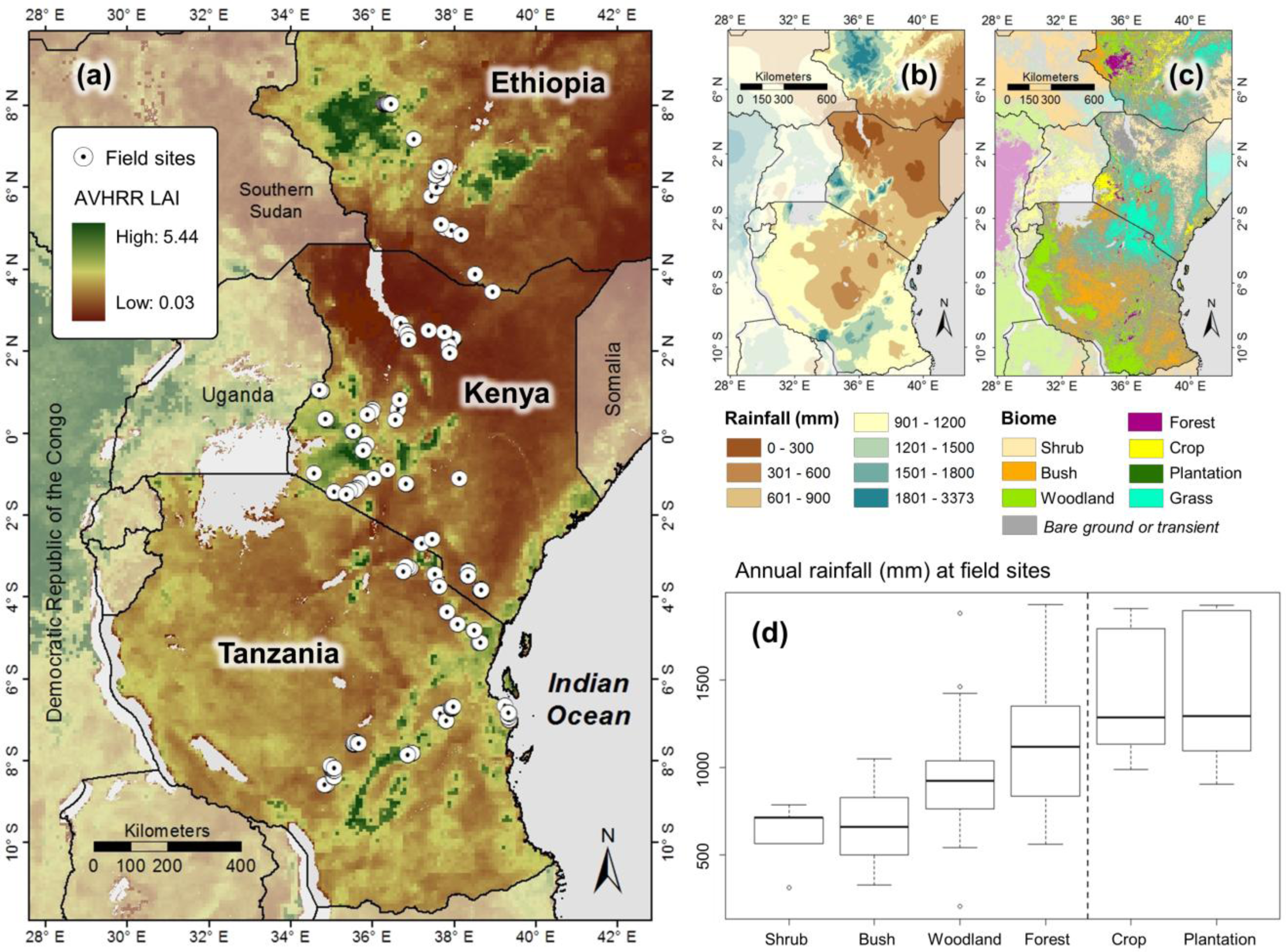
2.1. Study Region

Natural vegetation in East Africa (here defined as Tanzania, Kenya and Ethiopia) ranges from very open to very dense shrub (plants ≤ 2 m tall), deciduous bush of varying tree densities (plants 2–7 m tall), deciduous broad-leaved woodlands (plants > 7 m tall) of varying species compositions (e.g., Miombo in Tanzania and Acacia woodlands in Kenya and Ethiopia) and broadleaved semi-deciduous and evergreen forests (hereafter referred to as forests). As elsewhere in the tropics, these natural biomes are increasingly being degraded and converted to other land uses, particularly plantation and cropland. The primary drivers of land use change are high population growth and associated demand for land and resources, nationally and internationally [1820]. Pressure is higher near centers of demand, such as major towns, and in areas that are easier to access, such at low- to mid-altitudes, on flatter slopes, outside protected areas and close to roads [19,21]. Consequently, the majority of forest that remains is in mountainous regions, with villages often clustered around the foothills [18]. Drier, fire-prone woodlands and xeric low to high density bushlands dominate at lower altitudes, and are more susceptible to small-scale resource extraction (e.g., for charcoal production) and pressure from livestock grazing [7].

2.2. Ground-Measurements of LAI

We measured LAITrue at 274 sites across East Africa during ten field work campaigns, carried out between 2007 and 2012 (Figure 1, Table 1) following standard protocols [7,22]. At each site, we took high-resolution images through digital cameras equipped with hemispherical (fish-eye) lenses. The cameras were mounted on tripods at 1 m above ground, looking vertically upward from beneath the canopy [23]. The “levelled” hemispherical photographs were acquired normal to a local horizontal datum, orienting the optical axis of the lens to local zenith [24]. We measured under overcast conditions whenever possible to minimize anisotropy of the sky radiance [23]. On average, 19 images (median, 13) were taken at each site, distributed within plots according to VALERI design [25] (VAlidation of Land European Remote Sensing Instruments) or along linear north-south transects if field conditions required.
Hemispherical images were pre-processed by first extracting blue-channel pixel brightness values and then applying a threshold algorithm for separating sky from vegetation [26]. Resultant binary images were analyzed using the free canopy analysis software CAN-EYE V6.3.8 [27]. For each site, we derived LAI corrected for foliage element clumping [28], limiting the field of view of the lens to values between 0° and 60° to avoid mixed pixels.

2.3. Validation of GIMMS LAI3g

Direct validation of the LAIavhrr product with LAITrue was not possible, primarily because of the mismatch in spatial resolution between field data and AVHRR data [29]: each LAIavhrr pixel is likely to be a composite of different biomes, depending on the heterogeneity of the landscape. Instead, we indirectly validated LAIavhrr by comparing its distribution properties across biomes and environmental gradients with those properties for LAITrue. We thereby assume that the coarse resolution product is able to capture LAI variation and its underlying drivers at landscape scales.
First, we grouped LAIavhrr pixels belonging to a particular biome using MODIS land cover products for the years 2007 to 2011 (MCD12Q1v51 [30]), i.e., the time period of our field data, excluding those pixels that switched biome type during this time. We computed LAIavhrr as the average across the dry season months (December through February, June through August). Biomes of the MODIS land cover product were matched to biome types recorded in the field: evergreen broadleaf forest (=forest), deciduous broadleaf forest and woody savannas (=woodland), savannas (=bushland), closed and open shrublands (=shrubland), croplands and cropland/natural vegetation mosaic (=cropland), evergreen and deciduous needle-leaf forest (=plantation).
The geographic extent was set to the borders of Tanzania, Kenya and the southern part of Ethiopia, to match the regions sampled in the field. We created artificial “plots” using a random points generator, limiting the number of points within each biome to 1000. We specified a minimum distance of 8 km between points to minimise spatial autocorrelation and to exceed the pixel resolution of LAIavhrr maps. This algorithm created 80 plots in forest, 624 in woodland, 705 in bush, 995 in shrub and 294 in crop. Plantations are not well delimited within the MODIS land cover product and so the spatial extent of this biome was too low to generate a sufficient number of plots. For plantation only, we therefore increased the geographic extent to the west, thereby increasing the number of plantation “plots” to 11.
In a first step, we compared distribution properties of LAIavhrr and LAITrue for each biome. Secondly, we used generalised additive and general linear effects models to parameterise the responses of LAIavhrr and LAITrue to environmental gradients. Statistical analyses were carried out using R statistical software package [31].

2.4. LAI Response to Environmental Gradients

Rainfall and temperature estimates were extracted using WORLDCLIM interpolated climatology [32]. From these, we derived five weakly inter-correlated predictor variables (Table 2): mean annual rainfall (PPT), potential evapotranspiration (PET) [33] and an associated moisture index (MI = PPT/PET), precipitation of the driest quarter (PPT_DQ) and an associated moisture index for the driest quarter (MI_DQ), and annual temperature range (TE_R). For topographic predictors (elevation, ELEVATION, and slope, SLOPE), we used data from the 90 m spatial resolution Shuttle Radar Topographic Mission [34].
As a surrogate for the effects of natural grazing pressures on LAI, we used maps of herbivore browser richness (HERBIVORES) derived from International Union for Conservation of Nature range maps [35]. To quantify the effects of human pressures, we recorded whether a sampling site was located within or outside a protected area using the World Database on Protected Areas [36], calculated the (Euclidean) distance to roads (ROADS) and towns (TOWNS) using AFRICOVER data [37] and Open Street Map projects), and used maps of human population density (AFRIPOP [38,39]) to generate population pressure grids at 1 km spatial resolution (POPPRESS [40]). Pressure on a location i increases linearly with number of people p in a remote location j, such that POPPRESS i = j = 1 N p j w i j, where N is the number of locations across which the pressure accumulates. The weight w exerted by a remote population decreases exponentially with distance d, according to a half-normal distribution: wij = exp (−(dij/ơ)2). Increasing values of ơ increase the weight given to relatively distant populations. In exploratory analyses, ơ = 5 yielded the strongest correlation with LAI (testing ơ up to 25) and was used in all subsequent analyses.
The sample size (number of artificial plots) used for LAIavhrr was matched to the number of LAITrue plots measured for the respective biome in the field, so that statistical power was similar for LAIavhrr and LAITrue. LAIavhrr was subsetted for each biome (except forests and plantations) by randomly choosing samples 100 times. We then computed distance correlation statistics, DisR, using the dcor function (R package “energy”) to test for statistical dependence between LAITrue or LAIavhrr and each environmental predictor. We used the mean value of DisR across the 100 subsets of data. These analyses were repeated across and within biomes to account for potential biome-specific constraints masking relationships between biophysical structure and environmental drivers.
For subsequent analyses with general additive and general linear models, LAITrue and LAIavhrr were log-transformed to meet assumptions of normality. We included latitude and longitude as predictors to test for landscape-scale spatial autocorrelation. Models were fitted using Maximum Likelihood. Automated model selection was carried out using information theoretic approaches and multi-model averaging [41]. First, we constructed a global model including all predictors described above, except for moisture indices and PPD_DQ which were highly correlated with precipitation (Table 2). We then used the dredge function (R Package MuMIn v1.9.13), which constructs models using all possible combinations of the explanatory variables supplied in the global model. These models were ranked, relative to the “best” model, based on the change in Akaike Information Criterion (delta AIC). A multi-model average was calculated across all models with delta AIC < 2.

3. Results

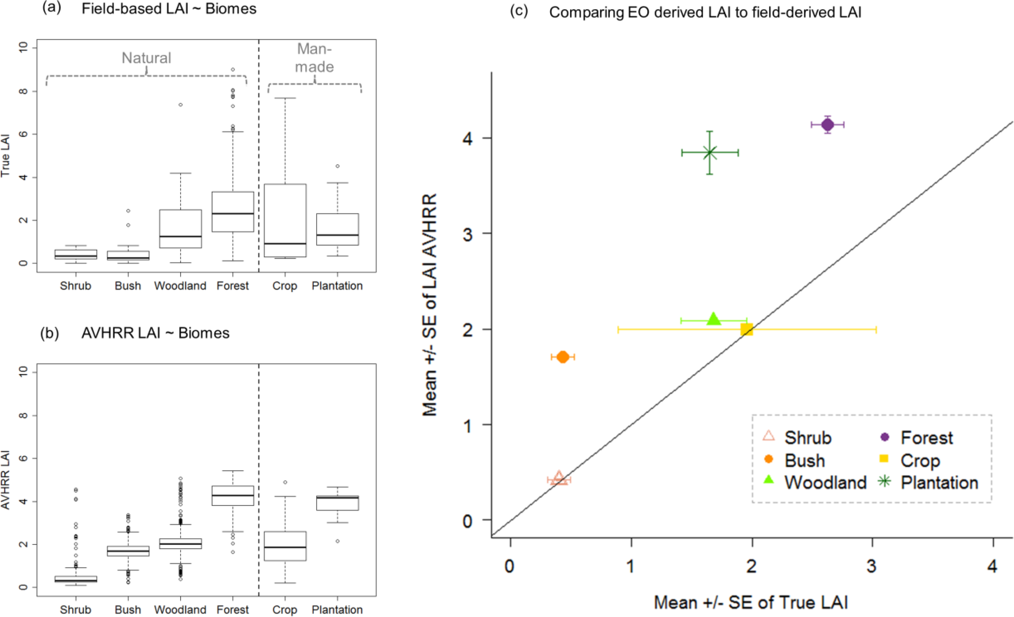
3.1. LAI Distribution within and between Biomes

LAITrue and LAIavhrr are not drawn from the same population, differing significantly in their medians, spread and shape (Mann-Whitney-Wilcox test: p < 0.001). LAITrue increased with vegetation height, from shrubland and bushland (similar) to woodland and then to forest (pairwise Wilcoxon tests, Bonferroni adjusted, p < 0.008; Table 3). Plantation had significantly lower LAITrue compared to forest, but significantly higher LAITrue compared to shrubland and bushland (Figure 2). LAIavhrr increased significantly with from shrubland to bush to woodland to forest (Table 3, Figure 2). Forest also had significantly higher LAIavhrr compared to plantation and cropland; which had significantly lower LAIavhrr than plantation. When comparing for each biome separately, LAIavhrr was significantly higher than LAITrue for forest, bushland, woodland and plantation (p < 0.001; Kruskal-Wallis tests), whilst being similar for cropland and shrubland.

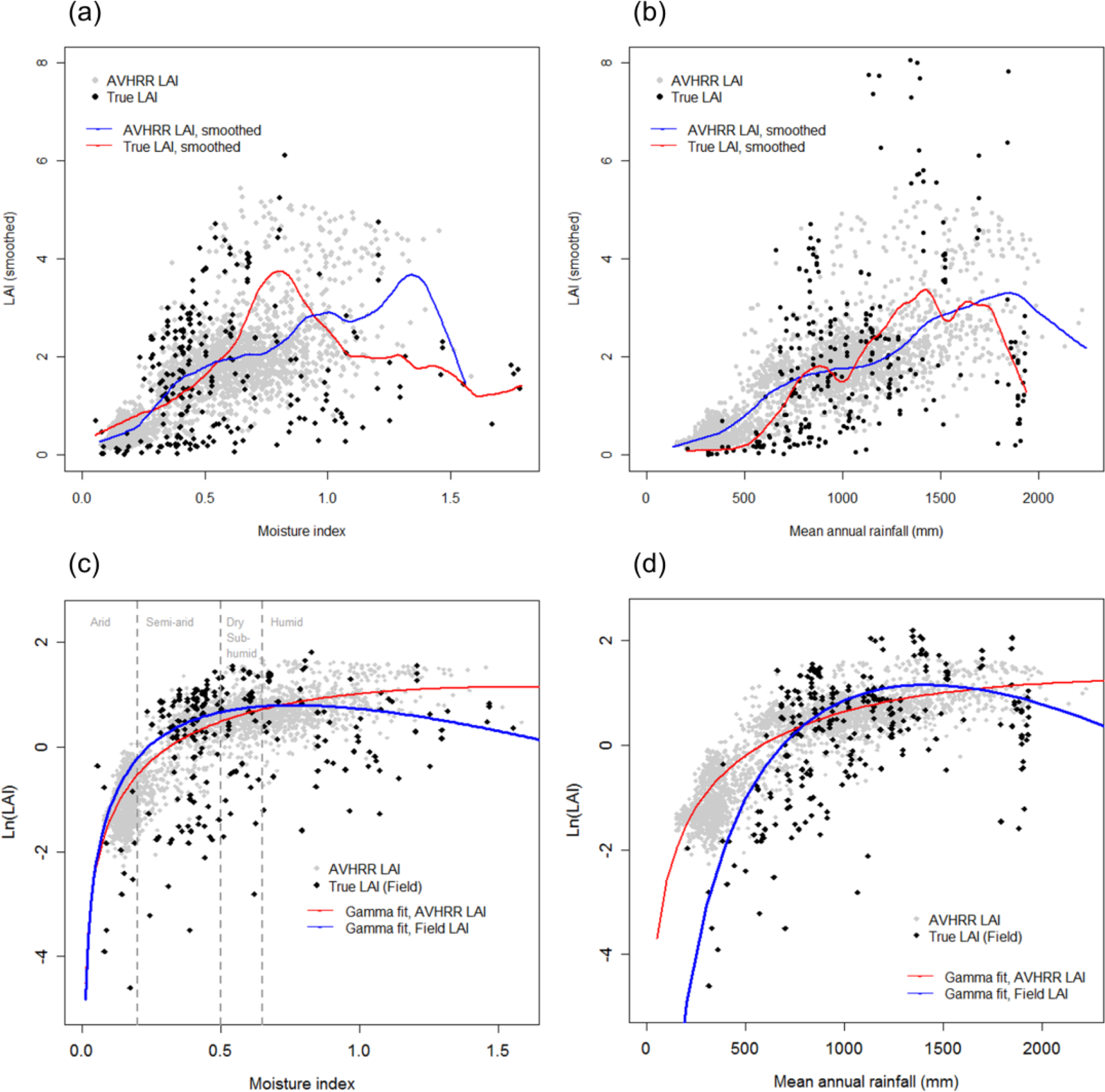
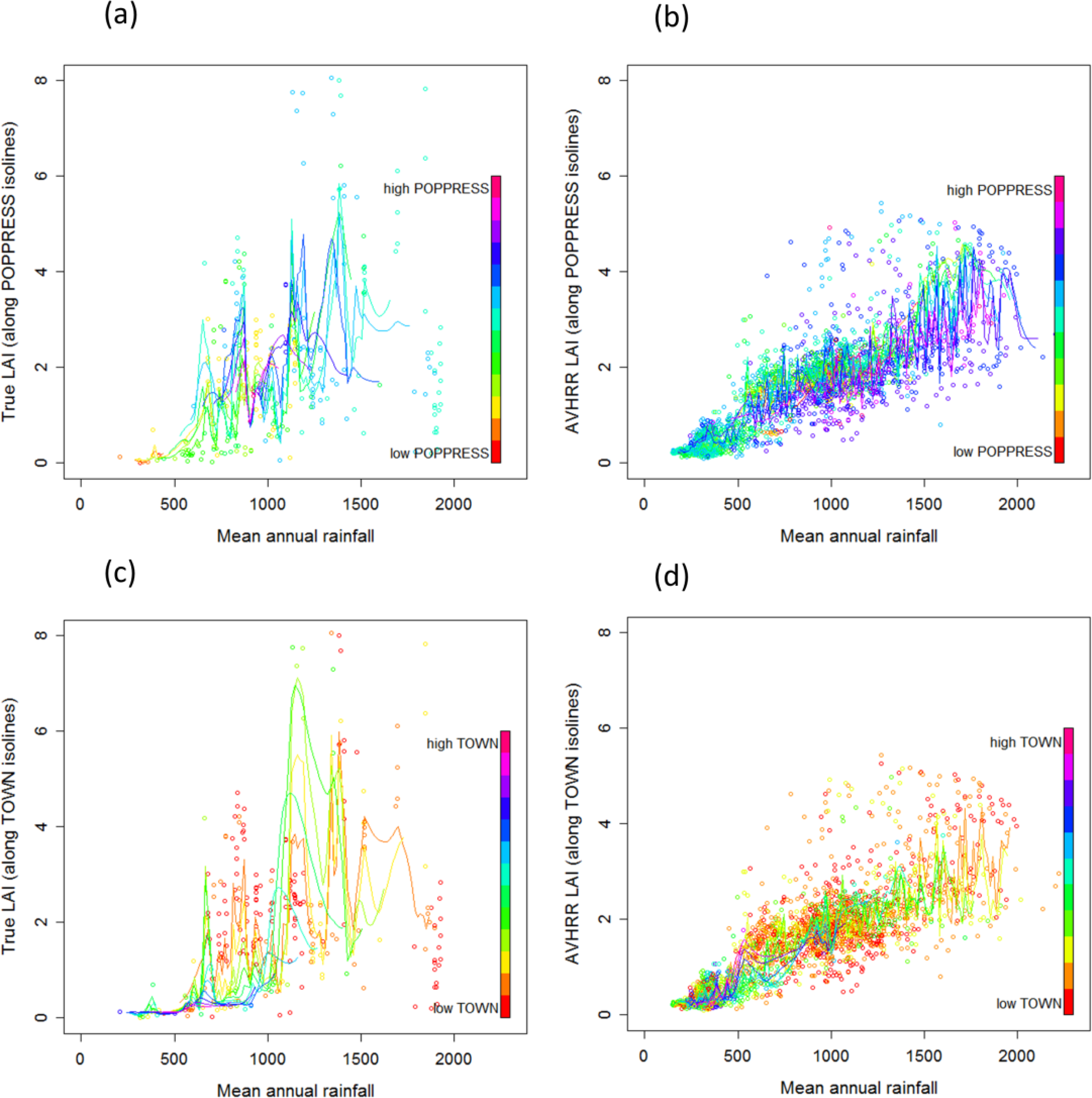
3.2. Distribution of LAI Response to Environmental Variation

Smoothed response curves of LAITrue and LAIavhrr versus PPT and MI were similar, showing an increase of LAI to global maxima, followed by a decrease at higher values of the environmental driver (Figure 3). Adhering to an a priori functional form, responses of LAITrue and LAIavhrr to PPT and MI were better captured by gamma distributions (Residual Standard Error, LAITrue: RSSPPT = 1.574, RSSMI = 0.584; LAIavhrr: RSSMI = 0.584, RSSPPT = 0.567) as opposed to logistic functions (LAITrue: RSSPPT = 1.609, RSSMI =1.18; LAIavhrr: did not converge) or linear models (LAITrue: RSSPPT = 1.676, RSSMI = 1.238; LAIavhrr: RSSMI = 0.600 and RSSPPT = 0.573).
Coefficients for parameters in the gamma fits (nls function R package “stats”) differed significantly between LAI estimates (Figure 3): the LAITrue response reached its maximum at lower values of the respective environmental driver and declines more strongly thereafter. LAITrue increased to 2.23 at MI = 0.76 mm and to 3.19 at PPT = 1400 mm decreasing thereafter, while LAIavhrr increased to 3.13 at MI = 1.58 and to 3.48 at PPT = 2700 mm decreasing thereafter.
Distance correlation statistics imply that both LAITrue and LAIavhrr are not completely independent of any of the environmental drivers tested (Table 4). The strength of the correlation between LAITrue and LAIavhrr and environmental drivers differs among biomes. Changes in the correlation strength between LAI and PPT, MI or HERBIVORES followed similar trends for LAITrue and LAIavhrr (Table 4). Yet, complex patterns emerged for other environmental drivers and field data showed more pronounced signals in responses to TOWNS, SLOPE and POPPRESS at biome level. PPT, POPPRESS and their interaction were all significant factors contributing to observed variability of LAITrue and LAIavhrr in general additive and general linear models (Table 5). Socio-economic variables contributed similarly to spatial variability in both LAITrue and LAIavhrr (Table 5). ROADS and TOWNS were significantly contributing to variability in LAITrue and LAIavhrr for both model types. LAI was higher within protected areas compared to unprotected land, and increased with SLOPE. However, general linear models identified fewer environmental predictors as contributing significantly to LAIavhrr variability compared to general additive models, suggesting a dominance of nonlinear relationships between environmental variables and LAI (Table 5).
We suspect the observed increase of LAI with increasing POPPRESS to be an indirect effect resulting from the increase of POPPRESS with PPT: i.e., P (LAI|PPT ∩ POPPRESS) similar to P (LAI|PPT). To visualize this conditional independence, we performed a triangulation-based natural neighbor interpolation of the 2D scattered data of LAI at PPT × POPPRESS locations using the Matlab function TriScatteredInterp.
This creates an interpolant that fits a surface of the form LAI = f (PPT, POPPRESS) which passes through the sample values at the point locations. We interpolated LAI on a regular grid of PPT × POPPRESS, which enabled us to look at variations of LAI with one variable whilst fixing the other one. Flat slopes in the rainfall isolines suggested that LAI given POPPRESS and PPT is indeed nearly the same as LAI given PPT only, although the curves indicate that LAI given high PPT is lower for high POPPRESS especially in the case of LAIavhrr (Figure 4). We also suspect the negative relationship between distance to town and LAI (Table 5) to be an indirect effect resulting from a saturation of LAI at higher rainfall, where many towns are located. Flat slopes of PPT isolines in response to TOWNS indicate conditional independence of LAI in response to TOWNS.

4. Discussion

The ultimate objective of linking EO data to biophysical land surface attributes (e.g., vegetation leaf area, biomass and productivity) is to characterize those attributes on large spatial scales and over time with minimal need for further fieldwork [42], so that the logistical, financial and subjective sampling constraints of fieldwork can be overcome. This requires that EO products, such as GIMMS LAI3g, accurately reflect conditions on the ground, both in absolute values and in their variation across space and time [43,44]. In this study, the increase in LAI with vegetation height for natural biomes (from shrubland/bushland to woodland and forest) is captured by both LAIavhrr and LAITrue. However, we find that LAIavhrr significantly overestimates LAI relative to LAITrue for all biomes except for shrubland and cropland. The coarse-spatial resolution of LAIavhrr may cause a bias towards the global mean of the region. Yet in East Africa, one would expect such a bias to result in lower LAI compared with estimates derived at high spatial resolution such as field-based LAITrue, because these landscapes are highly heterogeneous, and increasingly modified towards low LAI biomes such as degraded woodlands and crops. Moreover, LAIavhrr extracted from large tracts of homogeneous forest in Eastern Congo was found to be similar to LAIavhrr extracted for forests in our study area, again suggesting a consistent overestimation in the GIMMS LAI3g product.
In tropical Africa, vegetation phenology is particularly tuned to precipitation and its seasonal shifts [45,46], which may be impacted by rising global temperatures [47]. Rainfall triggers the emergence of green leaves in deciduous biomes, and controls vegetative growth and growth-duration in semi-arid and arid environments [48]. Vegetation indices such as NDVI, as a surrogate of vegetation productivity and phenology, have been linked to rainfall and rainfall and rainfall variability [49] in East Africa via a log-linear relationship. Nonlinear responses of LAI to PPT (and derived MI) in our study area are captured by both LAIavhrr and LAITrue by the same functional relationship. LAI increases with water availability up to a maximum, declining at higher values of annual rainfall and moisture. However, the response curves differ significantly, in that field-derived LAI reaches its maximum at lower values of the respective environmental driver, and exhibits a more rapid rate of change.
Further to climatic constraints, our analyses show that socio-economic factors play an important role in observed vegetation structure. LAI was found to be higher with increasing terrain steepness and within protected areas. These findings add evidence, based on biophysical structure, to previous studies showing how inaccessibility functions as a passive protection for woody biomes [18,19]. Our results are especially relevant for environmental management concerned with the maintenance of ecosystem processes and function, which are linked to biophysical properties such as LAI. Curiously, LAI was also found to be higher in regions under greater population pressure. Population pressure is greatest in areas of high rainfall, which are suitable for both crop production and high-LAI forest (of which there is less). Further, associated resource demands on adjacent woodlands and forests mean that, in many areas, these biomes have degraded to bushland and shrubland, which may exhibit higher biome-specific LAI than rainfall-limited bushland and shrubland elsewhere. Thus the observed pattern may reflect historical land use impacts rather than a positive causal relationship between human population pressure and vegetation leaf area. A visual comparison of LAI rainfall isolines along a gradient of increasing population pressure shows primarily flat slopes, supporting the above hypothesis. This pattern is especially apparent in the LAIavhrr response and, if at all, there seems to be a negative effect of increasing population pressure on LAI in regions with high rainfall.
Validating coarse-scale spatial resolution data with field measurements is inherently difficult due to challenges of spatial mismatch [50] and differing spatial scales [51]. LAI distributions inferred from field measurement and satellite retrieval should ideally converge to the true intrinsic distribution of the vegetation class in a given region at a given time [52]. Whilst our findings are encouraging regarding the capacity of EO data to capture spatial variation in LAI along major environmental gradients, they also highlight the need for further field assessments of inter- and intra-annual LAI dynamics, especially in remote woody biomes, in croplands and in plantations. An important issue, arising from our use of MODIS land cover products in the generation of biome-specific random plots, is that plantations are difficult to distinguish from natural forests, especially if consisting of broadleaved evergreen trees. We find that very few plantations are identified by the MODIS product, despite large areas of forests being converted to plantations in both Kenya and Ethiopia. Similarly, spectral similarities complicate the distinction between “woody savanna” and savanna, as well as between grassland and cropland [30], particularly when the latter are rotated in seasonal succession rather than being left fallow. It is encouraging, however, that despite these uncertainties in biome-specific LAIavhrr estimates, the increase in LAI with vegetation height is captured by LAIavhrr and LAITrue similarly. Furthermore, general additive models identified the same set of environmental predictors having similar impacts on both LAI estimates.

5. Conclusions

Remotely sensed, global-scale estimates of biophysical structure, such as LAIavhrr effectively capture spatial variation in LAI along major environmental gradients, but some challenges remain. First, LAIavhrr appears to consistently overestimate LAI in woody biomes such as forest. Second, nonlinear responses of LAI to water availability, while captured by both LAIavhrr and LAITrue similarly, differ significantly in their parameterization, such that the remotely sensed product reaches its maximum at higher values of rainfall and moisture index than field-derived LAITrue suggests may be the case. LAITrue increased to 2.23 at MI = 0.76 mm and to 3.19 at PPT = 1400 mm decreasing thereafter, while LAIavhrr increased to 3.13 at MI = 1.58 and to 3.48 at PPT = 2700 mm decreasing thereafter. Third, distance correlation statistics show significant relationships with all environmental drivers tested for both LAITrue and LAIavhrr, although the strength of that correlation varies between LAITrue and LAIavhrr responses.
More generally, we find that the same set of environmental drivers emerges as significant in models of LAI variability. Beside rainfall, temperature and topography, socio-economic correlates such as population pressure, distance to roads, distance to towns and protection status are important for understanding spatial variation of vegetation biophysical structure in the human-modified landscapes of tropical Africa. The responses to these drivers are largely consistent for LAIavhrr and LAITrue except for their responses to potential evapotranspiration. Note though, that protection status, rainfall, temperature range and topography were not significant in general linear models of LAIavhrr variability despite being significant in general additive models suggesting complex underlying relationships.
In particular, higher forest LAI observed within the protected area network suggests a potential mechanism for monitoring efforts to reduce forest degradation (e.g., for carbon conservation or catchment protection). Given the above challenges, targeted field measurements, stratified according to both environmental and socio-economic gradients, will be needed to improve the accuracy of satellite-derived estimates.

Acknowledgments

MP was supported by the Marie Curie Intra-European fellowship IEF Programme (EU FP7-People-IEF-2008 Grant Agreement No. 234394) and is now supported by the European Research Council Project No. 281986. PJP, RAM and PKEP are supported by the Ministry for Foreign Affairs of Finland through the CHIESA Project ( http://chiesa.icipe.org/). We acknowledge the British Institute in East Africa for logistic support, Simon Willcock (SW in Table 2), Lena Jeha (LJ) and Aida Cuni-Sanchez (ACS) for help during field work, and Jonathan Green for sharing R code. We warmly thank Hamidu Seki (HS) and the WWF-TZ REDD+ project (funded by the Norwegian government) for providing some of the hemispherical images (ID07) used in this study. We thank four anonymous reviewers for their comments which helped to improve the manuscript. This paper is a contribution to Imperial College’s Grand Challenges in Ecosystems and the Environment initiative.

Author Contributions

Marion Pfeifer and Philip Platts conceived the study, collected field data, performed the analyses and prepared the manuscript. Veronique Lefebvre contributed to statistical analyses and interpretation of results. Petri Pellikka, Rob Marchant and Alemu Gonsamo contributed field data and helped with manuscript revisions. Dereje Denu contributed data from the Jimma Highlands in Ethiopia.

Conflicts of Interest

The authors declare no conflict of interest.

References

  1. Chen, J.M.; Pavlic, G.; Brown, L.; Cihlar, J.; Leblanc, S.; White, H.; Hall, R.; Peddle, D.; King, D.; Trofymow, J.; et al. Derivation and validation of Canada-wide coarse-resolution leaf area index maps using high-resolution satellite imagery and ground measurements. Remote Sens. Environ 2002, 80, 165–184. [Google Scholar]
  2. Sabater, J.M.; Rüdiger, C.; Calvet, J.C.; Fritz, N.; Jarlan, L.; Kerr, Y. Joint assimilation of surface soil moisture and LAI observations into a land surface model. Agric. For. Meteorol 2008, 148, 1362–1373. [Google Scholar] [Green Version]
  3. Sellers, P.; Dickinson, R.; Randall, D.; Betts, A.; Hall, F.; Berry, J.; Collatz, G.; Denning, A.; Mooney, H.; Nobre, C.; et al. Modeling the exchanges of energy, water, and carbon between continents and the atmosphere. Science 1997, 275, 502–509. [Google Scholar]
  4. Launay, M.; Guérif, M. Ability for a model to predict crop production variability at the regional scale: An evaluation for sugar beet. Agronomie 2003, 23, 135–146. [Google Scholar]
  5. Neitsch, S.; Arnold, J.; Kiniry, J.; Williams, J.; King, K. Soil and Water Assessment Tool: Theoretical Documentation Version 2005; Blackland Research Centre: Temple, TX, USA, 2005. [Google Scholar]
  6. Matricardi, E.A.; Skole, D.L.; Pedlowski, M.A.; Chomentowski, W.; Fernandes, L.C. Assessment of tropical forest degradation by selective logging and fire using Landsat imagery. Remote Sens. Environ 2010, 114, 1117–1129. [Google Scholar]
  7. Pfeifer, M.; Gonsamo, A.; Disney, M.; Pellikka, P.; Marchant, R. Leaf area index for biomes of the Eastern Arc Mountains: Landsat and SPOT observations along precipitation and altitude gradients. Remote Sens. Environ 2012, 118, 103–115. [Google Scholar]
  8. Fang, H.; Jiang, C.; Li, W.; Wei, S.; Baret, F.; Chen, J.M.; Garcia-Haro, J.; Liang, S.; Liu, R.; Myneni, R.B.; et al. Characterization and intercomparison of global moderate resolution leaf area index (LAI) products: Analysis of climatologies and theoretical uncertainties. J. Geophys. Res.: Biogeosci 2013, 118, 529–548. [Google Scholar]
  9. Myneni, R.; Hoffman, S.; Knyazikhin, Y.; Privette, J.; Glassy, J.; Tian, Y.; Wang, Y.; Song, X.; Zhang, Y.; Smith, G.; et al. Global products of vegetation leaf area and fraction absorbed PAR from year one of MODIS data. Remote Sens. Environ 2002, 83, 214–231. [Google Scholar]
  10. Baret, F.; Hagolle, O.; Geiger, B.; Bicheron, P.; Miras, B.; Huc, M.; Berthelot, B.; Niño, F.; Weiss, M.; Samain, O.; et al. LAI, fAPAR and fCover CYCLOPES global products derived from VEGETATION: Part 1: Principles of the algorithm. Remote Sens. Environ 2007, 110, 275–286. [Google Scholar]
  11. Myneni, R.B.; Ramakrishna, R.; Nemani, R.; Running, S. Estimation of global leaf area index and absorbed PAR using radiative transfer models. IEEE Trans. Geosci. Remote Sens 1997, 35, 1380–1393. [Google Scholar]
  12. Fernandes, R.; Butson, C.; Leblanc, S.; Latifovic, R. Landsat-5 TM and Landsat-7 ETM+ based accuracy assessment of leaf area index products for Canada derived from SPOT-4 VEGETATION data. Can. J. Remote Sens 2003, 29, 241–258. [Google Scholar]
  13. Myneni, R.B.; Hall, F.G.; Sellers, P.J.; Marshak, A.L. The interpretation of spectral vegetation indexes. IEEE Trans. Geosci. Remote Sens 1995, 33, 481–486. [Google Scholar]
  14. Zhu, Z.; Bi, J.; Pan, Y.; Ganguly, S.; Anav, A.; Xu, L.; Samanta, A.; Piao, S.; Nemani, R.R.; Myneni, R.B. Global data sets of vegetation leaf area index (LAI) 3g and Fraction of Photosynthetically Active Radiation (FPAR) 3g derived from Global Inventory Modeling and Mapping Studies (GIMMS) Normalized Difference Vegetation Index (NDVI3g) for the period 1981 to 2011. Remote Sens 2013, 5, 927–948. [Google Scholar]
  15. Mao, J.; Shi, X.; Thornton, P.E.; Hoffman, F.M.; Zhu, Z.; Myneni, R.B. Global latitudinal-asymmetric vegetation growth trends and their driving mechanisms: 1982–2009. Remote Sens 2013, 5, 1484–1497. [Google Scholar]
  16. Cook, B.I.; Pau, S. A global assessment of long-term greening and browning trends in pasture lands using the GIMMS LAI3g dataset. Remote Sens 2013, 5, 2492–2512. [Google Scholar]
  17. Pfeifer, M.; Platts, P.J. Ground Measurements of Leaf Area Index in Africa, Version 1.5. 2014. Available online: http://www.york.ac.uk/environment/research/kite/resources/ (accessed on 29 January 2014).
  18. Green, J.M.; Larrosa, C.; Burgess, N.D.; Balmford, A.; Johnston, A.; Mbilinyi, B.P.; Platts, P.J.; Coad, L. Deforestation in an African biodiversity hotspot: Extent, variation and the effectiveness of protected areas. Biol. Conserv 2013, 164, 62–72. [Google Scholar]
  19. Pfeifer, M.; Burgess, N.D.; Swetnam, R.D.; Platts, P.J.; Willcock, S.; Marchant, R. Protected areas: Mixed success in conserving East Africa’s evergreen forests. PLoS One 2012, 7, e39337. [Google Scholar] [CrossRef]
  20. Pfeifer, M.; Platts, P.J.; Burgess, N.D.; Swetnam, R.D.; Willcock, S.; Lewis, S.L.; Marchant, R. Land use change and carbon fluxes in East Africa quantified using earth observation data and field measurements. Environ. Conserv 2013, 40, 242–252. [Google Scholar]
  21. Platts, P.J.; Burgess, N.D.; Gereau, R.; Lovett, J.; Marshall, A.R.; McCLEAN, C.J.; Pellikka, P.K.; Swetnam, R.D.; Marchant, R. Delimiting tropical mountain ecoregions for conservation. Environ. Conserv 2011, 38, 312–324. [Google Scholar]
  22. Zhang, Y.; Chen, J.M.; Miller, J.R. Determining digital hemispherical photograph exposure for leaf area index estimation. Agric. For. Meteorol 2005, 133, 166–181. [Google Scholar]
  23. Jonckheere, I.; Fleck, S.; Nackaerts, K.; Muys, B.; Coppin, P.; Weiss, M.; Baret, F. Review of methods for in situ leaf area index determination: Part I. Theories, sensors and hemispherical photography. Agric. For. Meteorol 2004, 121, 19–35. [Google Scholar]
  24. Gonsamo, A.; Pellikka, P. Methodology comparison for slope correction in canopy leaf area index estimation using hemispherical photography. For. Ecol. Manag 2008, 256, 749–759. [Google Scholar]
  25. VALERI. Available online: http://w3.avignon.inra.fr/valeri (accessed on 10 August 2013).
  26. Jonckheere, I.; Muys, B.; Coppin, P. Allometry and evaluation of in situ optical LAI determination in Scots pine: A case study in Belgium. Tree Physiol 2005, 25, 723–732. [Google Scholar]
  27. Weiss, M.; Baret, F. CAN-EYE V6. 1 USER MANUAL. 2010. Available online: http://www6.paca.inra.fr/can-eye/Download (accessed on 29 January 2014).
  28. Weiss, M.; Baret, F.; Myneni, R.B.; Pragnère, A.; Knyazikhin, Y. Investigation of a model inversion technique to estimate canopy biophysical variables from spectral and directional reflectance data. Agronomie 2000, 20, 3–22. [Google Scholar]
  29. Garrigues, S.; Lacaze, R.; Baret, F.; Morisette, J.; Weiss, M.; Nickeson, J.; Fernandes, R.; Plummer, S.; Shabanov, N.; Myneni, R.B.; et al. Validation and intercomparison of global Leaf Area Index products derived from remote sensing data. J. Geophys. Res.: Biogeosci 2008, 113. [Google Scholar] [CrossRef]
  30. Friedl, M.A.; Sulla-Menashe, D.; Tan, B.; Schneider, A.; Ramankutty, N.; Sibley, A.; Huang, X. MODIS Collection 5 global land cover: Algorithm refinements and characterization of new datasets. Remote Sens. Environ 2010, 114, 168–182. [Google Scholar]
  31. Team, R.C. R: A Language and Environment for Statistical Computing; R Foundation for Statistical Computing: Vienna; Available online: http://www.r-project.org/ (accessed on 1 September 2013).
  32. Hijmans, R.J.; Cameron, S.E.; Parra, J.L.; Jones, P.G.; Jarvis, A. Very high resolution interpolated climate surfaces for global land areas. Int. J. Climatol 2005, 25, 1965–1978. [Google Scholar]
  33. Hargreaves, G.; Allen, R. History and evaluation of Hargreaves evapotranspiration equation. J. Irrig. Drain. Eng 2003, 129, 53–63. [Google Scholar]
  34. Rodriguez, E.; Morris, C.S.; Belz, J.E. A global assessment of the SRTM performance. Photogramm. Eng. Remote Sens 2006, 72, 249–260. [Google Scholar]
  35. Greve, M.; Lykke, A.M.; Fagg, C.W.; Bogaert, J.; Friis, I.; Marchant, R.; Marshall, A.R.; Ndayishimiye, J.; Sandel, B.S.; Sandom, C.; et al. Continental-scale variability in browser diversity is a major driver of diversity patterns in acacias across Africa. J. Ecol 2012, 100, 1093–1104. [Google Scholar]
  36. IUCN; UNEP-WCMC. The World Database on Protected Areas (WDPA); UNEP-WCMC: Cambridge, UK, 2010; Available online: http://www.protectedplanet.net (accessed on 29 October 2013).
  37. GeoNetwork. Available online: http://www.fao.org/geonetwork/ (accessed on 10 July 2013).
  38. Linard, C.; Gilbert, M.; Snow, R.W.; Noor, A.M.; Tatem, A.J. Population distribution, settlement patterns and accessibility across Africa in 2010. PLoS One 2012, 7, e31743. [Google Scholar] [CrossRef]
  39. Tatem, A.J.; Noor, A.M.; von Hagen, C.; di Gregorio, A.; Hay, S.I. High resolution population maps for low income nations: Combining land cover and census in East Africa. PLoS One 2007, 2, e1298. [Google Scholar] [CrossRef]
  40. Platts, P.J. Spatial Modelling, Phytogeography and Conservation in the Eastern Arc Mountains of Tanzania and Kenya. Ph.D. Thesis, Environment Department, University of York, York, UK. 2012. [Google Scholar]
  41. Grueber, C.; Nakagawa, S.; Laws, R.; Jamieson, I. Multimodel inference in ecology and evolution: Challenges and solutions. J. Evol. Biol 2011, 24, 699–711. [Google Scholar]
  42. Kalácska, M.; Sánchez-Azofeifa, G.A.; Rivard, B.; Calvo-Alvarado, J.C.; Journet, A.; Arroyo-Mora, J.P.; Ortiz-Ortiz, D. Leaf area index measurements in a tropical moist forest: A case study from Costa Rica. Remote Sens. Environ 2004, 91, 134–152. [Google Scholar]
  43. Van Leeuwen, W.J.D.; Orr, B.J.; Marsh, S.E.; Herrmann, S.M. Multi-sensor NDVI data continuity: Uncertainties and implications for vegetation monitoring applications. Remote Sens. Environ 2006, 100, 67–81. [Google Scholar]
  44. Morisette, J.T.; Baret, F.; Privette, J.L.; Myneni, R.B.; Nickeson, J.E.; Garrigues, S.; Shabanov, N.V.; Weiss, M.; Fernandes, R.A.; Leblanc, S.G.; et al. Validation of global moderate-resolution LAI products: A framework proposed within the CEOS land product validation subgroup. IEEE Trans. Geosci. Remote Sens 2006, 44, 1804–1817. [Google Scholar]
  45. Davenport, M.; Nicholson, S. On the relation between rainfall and the normalized difference vegetation index for diverse vegetation types in East Africa. Int. J. Remote Sens 1993, 14, 2369–2389. [Google Scholar]
  46. Herrmann, S.M.; Anyamba, A.; Tucker, C.J. Recent trends in vegetation dynamics in the African Sahel and their relationship to climate. Glob. Environ. Chang 2005, 15, 394–404. [Google Scholar]
  47. Pachauri, R.K. Climate Change 2007. Synthesis Report; Contribution of Working Groups I, II and III to the Fourth Assessment Report; Cambridge University Press: Cambridge, UK/New York, NY, USA, 2008. [Google Scholar]
  48. Zhang, X.; Friedl, M.A.; Schaaf, C.B.; Strahler, A.H.; Liu, Z. Monitoring the response of vegetation phenology to precipitation in Africa by coupling MODIS and TRMM instruments. J. Geophys. Res.: Atmos 2005, 110. [Google Scholar] [CrossRef]
  49. Nicholson, S.; Farrar, T. The influence of soil type on the relationships between NDVI, rainfall, and soil moisture in semiarid Botswana. I. NDVI response to rainfall. Remote Sens. Environ 1994, 50, 107–120. [Google Scholar]
  50. Tan, B.; Woodcock, C.; Hu, J.; Zhang, P.; Ozdogan, M.; Huang, D.; Yang, W.; Knyazikhin, Y.; Myneni, R.B. The impact of gridding artifacts on the local spatial properties of MODIS data: Implications for validation, compositing, and band-to-band registration across resolutions. Remote Sens. Environ 2006, 105, 98–114. [Google Scholar]
  51. Wang, Y.; Woodcock, C.E.; Buermann, W.; Stenberg, P.; Voipio, P.; Smolander, H.; Häme, T.; Tian, Y.; Hu, J.; Knyazikhin, Y.; et al. Evaluation of the MODIS LAI algorithm at a coniferous forest site in Finland. Remote Sens. Environ 2004, 91, 114–127. [Google Scholar]
  52. Buermann, W.; Wang, Y.; Dong, J.; Zhou, L.; Zeng, X.; Dickinson, R.E.; Potter, C.S.; Myneni, R.B. Analysis of a multiyear global vegetation leaf area index data set. J. Geophys. Res.: Atmos 2002, 107. [Google Scholar] [CrossRef]
Figure 1. Distribution of 274 field sites in relation to the Global Inventory Modeling and Mapping Studies (GIMMS) LAI3g product, rainfall and major biome types in East Africa. (a) Distribution of field sites located in shrub, bush, woodland, forest, crops and plantations overlaid on Earth Observation (EO) derived LAIavhrr map (for details see Text). (b) Rainfall environment in East Africa derived from WORLDCLIM (1 km pixel resolution). (c) Distribution of biome pixels with no change in biome between 2007 and 2011. (d) Rainfall environment of field sites.
Remotesensing 06 01973f1
Figure 2. Estimates of field-derived LAI (LAITrue) and earth observation-derived LAI (LAIavhrr) for natural and man-made biomes in East Africa. (a) LAITrue estimates derived for 274 study sites. (b) LAIavhrr estimates derived for randomly created plots using MODIS biome maps. (c) Comparison between LAIavhrr and LAITrue (1:1 line indicates complete agreement).
Remotesensing 06 01973f2
Figure 3. Nonlinear responses of LAITrue and LAIavhrr to annual rainfall (PPT) and moisture index (MI). Smoothed curves (local regression of 10% of points with weighted linear least squares) of LAI responses to gradients of MI (a) and PPT (b) summarize patterns without imposing a priori functional forms. In (c,d) gamma fits (y = A × (x(k − 1) × exp(−x/s))/(sk × gamma(k))) are displayed using a natural logarithmic for the y-scale. LAITrue response reaches its maximum at lower values of the respective environmental driver compared to LAIavhrr response and declines more strongly thereafter.
Remotesensing 06 01973f3
Figure 4. Population pressure (POPPRESS) and distance to town (TOWN) isolines of LAI in response to increasing annual rainfall (PPT) for LAITrue and LAIavhrr. (a,b) For a given level of rainfall, LAI does not depend on the level of POPPRESS. However, in high rainfall regions, high levels of POPPRESS have a noticeable negative impact on LAI, which is especially apparent in the LAIavhrr response. (c,d) Isolines suggest conditional independence of LAI and TOWN. However, there are no data with the combination of high TOWN and high rainfall, thus conclusions in the range of these parameter combinations are highly uncertain.
Remotesensing 06 01973f4
Table 1. Ten field campaigns (ID) were carried out between 2007 and 2012. Hemispherical images were taken in 20 m × 20 m plots or along linear transects depending on environmental conditions in the field. N—Number of plots or transects measured (plots including fewer than eight sample points were excluded from analyses). Country—Field campaigns took place in Ethiopia (ETH), Kenya (KEN) and Tanzania (TZA). PI—Main coordinator of field work campaign.
IDNDateCountryCameraLensPI
ID0137January 2010TZA, KENNikon D5000Nikkor F2.8MP, RAM
ID0243July 2010TZACanon EOS 450DSigma 4.5 F2.8MP, SW *
ID0358January 2010KENNikon D5000 SLRSigma 4.5 F2.8PKEP
ID0423January 2007KENNikon 8800 VRNikon FC-E9AG
ID0531June 2011KENCanon EOS 450DSigma 4.5 F2.8MP, ACS *
ID0632June 2012KEN, ETHNikon D3100Sigma 4.5 F2.8MP, PJP, ACS *
ID06a8June 2012ETHNikon D5000Nikkor F2.8RAM
ID0720August 2011TZANikon D3100Sigma 4.5 F2.8HS *
ID0811November 2012KENNikon D800Sigma 4.5 F2.8RAM
ID1031May to June 2012KENNikon D800Sigma 4.5 F2.8MP, RAM, PJP, LJ *
ID1214June 2012ETHNikon D5000Nikkor F2.8DD
*See Acknowledgements.
Table 2. Pearson’s product moment correlation coefficients (Spearman’s rho) between predictor variables for the field derived point data. NS—correlation not significant at p = 0.05. 1—Mean Annual Precipitation, 2—Potential Evapotranspiration, 3—Moisture Index, 4—Temperature Range, 5—Precipitation driest quarter, 6—Moisture index for driest quarter, 7—Population pressure, 8—SRTM Slope, 9—SRTM Elevation, 10—Herbivore Browser Richness, 11—Distance to Roads, 12—Distance to Towns. NS: correlation not significant. Cell entries: spearman’s rho estimates. Bold values indicate values above the correlation threshold of 0.6.
1234567891011
2−0.39-
30.64NS-
4−0.160.800.13
50.64−0.140.52NS-
60.57NS0.53NS0.91
70.48NS0.470.190.180.18-
8NS−0.31−0.13−0.370.13NS−0.29-
90.42−0.220.380.280.380.310.43NS-
10−0.26−0.14−0.41−0.15−0.19−0.24−0.260.29NS-
110.25NS0.360.160.16NSNSNS0.23−0.14-
12−0.17NSNS0.12−0.25−0.28NS−0.45nsns−0.21
Table 3. LAITrue was measured within plots or along transects in the field (FI) using hemispherical photography. LAIavhrr was extracted from the earth observation-derived GIMMS LAIg3 product (EO, biome-specific plots randomly created in GIS). Shaded cells: LAI estimates differed significantly between FI and EO (Kruskal-Wallis test, p < 0.001). Statistical properties of LAI distributions: Mean ± Standard Error, Median, Interquartile range (IQR), and Maximum.
NumberMean ± SEMedianIQRMax

FIEOFIEOFIEOFIEOFIEO
Shrub99950.4 ± 0.10.4 ± 0.00.40.30.40.30.84.6
Bush297050.4 ± 0.11.7 ± 0.00.31.70.40.52.53.4
Woodland326241.7 ± 0.32.1 ± 0.01.32.01.70.57.45.1
Forest174802.6 ± 0.14.1 ± 0.12.34.31.80.99.05.4
Crop72942.0 ± 1.12.0 ± 0.10.51.92.31.37.74.9
Plantation23111.6 ± 0.23.8 ± 0.21.34.21.50.74.54.7
Table 4. Response of satellite-derived LAIavhrr (EO) and field-derived LAITrue (FI) to environmental gradients in single-predictor models, according to distance correlations (0 < DisR < 1, where DisR∼0 indicates independence). Highlights indicate that DisR for LAITrue and LAIavhrr differed by more than 0.1 (green) or by more than 0.2 (purple), in which cases we assume that the relationship between LAITrue and environmental predictor is different from the relationship between LAIavhrr and the environmental predictor.
PPTMIPETPOP-PRESSSlopeHERBMI_DQPPT_DQTOWNELE-VATIONROADSTR

FIEOFIEOFIEOFIEOFIEOFIEOFIEOFIEOFIEOFIEOFIEOFIEO
Shrub0.860.640.760.640.760.570.720.540.780.590.410.600.430.600.540.590.670.530.840.590.340.490.390.53
Bush0.490.520.430.490.260.390.650.350.760.330.380.410.300.440.390.450.480.360.360.380.250.330.300.38
Wood0.350.530.480.490.400.420.330.310.360.410.400.370.600.550.510.540.450.350.320.420.310.320.350.35
Forest0.390.170.270.170.310.360.390.190.250.140.370.250.220.230.410.270.300.160.220.220.120.190.290.19
Crop0.550.550.580.480.850.270.530.280.690.250.470.440.510.670.700.680.510.240.690.610.460.550.650.59
Plantation0.420.400.360.360.380.390.470.530.290.450.450.360.560.560.470.550.370.630.400.460.430.540.400.44
All0.400.660.230.640.360.410.330.510.320.480.230.480.180.660.320.660.390.460.160.590.140.390.330.40
Table 5. Relative Variable Importance (RVI) in general linear and general additive models (GLM and GAM) of field- and satellite-derived LAI in response to environmental predictors. RVI is calculated for each predictor by summing the AIC weights across all models where the variable occurs (models of interest are determined by delta AIC < 2; see main text). Because of high correlation between moisture indices and precipitation (Table 2), we excluded the former from global models. GLMs are first order unless superscripted (a) in which case second order. Smooth terms in GAMs were allowed two effective degrees of freedom. For second order GLMs, signs for coefficients are given for first (P1) and second-order polynomial (P2).
RVI; LAITrue ModelsRVI; LAIavhrr ModelsSign of Estimated GLM Coefficients

GAMGLMGAMGLMFieldEO
Biome type1.01.01.01.0PositivePositive
Mean annual rainfall (PPT)0.491.0 a0.50P1: +; P2: −
Potential evapotranspiration0.500.281.00.22NegativePositive
Temperature range0.330.611.0Negative
Population pressure (POPPRESS)0.531.01.00.30PositivePositive
Distance to roads0.200.120.321.0PositivePositive
Distance to towns1.00.111.00.57NegativeNegative
Protected1.01.01.0Positive
Elevation1.01.01.0Negative
Slope0.621.01.0Positive
Latitude/Longitude1.01.01.01.0PositivePositive
PPT × POPPRESS1.0-1.0-
Biomes:Slope-1.0--
AIC479.5–481.4591.1–593.1912.6–914.1−112.3–−110.4

