Article

Assessing the Robustness of Vegetation Indices to Estimate Wheat N in Mediterranean Environments

1
Department of Agricultural & Biological Engineering, University of Florida, Gainesville, FL 32611, USA
2
Department of Primary Industries, 110 Natimuk Rd., Horsham 3401, Australia
3
Department of Crop Production, Universita' della Tuscia, Viterbo 01100, Italy
4
Department of Geological Sciences, Michigan State University, East Lansing, MI 48824, USA
*
Author to whom correspondence should be addressed.
Remote Sens. 2014, 6(4), 2827-2844; https://doi.org/10.3390/rs6042827
Submission received: 7 January 2014 / Revised: 19 March 2014 / Accepted: 20 March 2014 / Published: 27 March 2014

Abstract

:
Remotely sensed vegetation indices have been extensively used to quantify plant and soil characteristics. The objectives of this study were to: (i) compare vegetation indices developed at different scales for measuring canopy N content (g·N·m−2) and concentration (%); and (ii) evaluate the effects of soil background reflectance, cultivar, illumination and atmospheric conditions on the ability of vegetation indices to estimate canopy N content. Data were collected from two rainfed field sites cropped to wheat in Southern Italy (Foggia) and in Southeastern Australia (Horsham). From spectral readings, 25 vegetation indices were calculated. The Perpendicular Vegetation Index showed the best prediction of plant N concentration (%) (r2 = 0.81; standard error (SE) = 0.41%; p < 0.001). The Canopy Chlorophyll Content Index showed the best predictive capability for canopy N content (g·N·m−2) (r2 = 0.73; SE = 0.603; p < 0.001). Canopy N content was best related to indices developed at the canopy scale and containing a red-edge wavelength. Canopy-scale indices were related to canopy N%, but such relationships needed to be normalized with biomass. Geographical location influenced mainly simple ratio or normalized indices, while indices that contained red-edge wavelengths were more robust and able to estimate canopy parameters more accurately.

1. Introduction

Vegetation indices (VIs) based on spectral reflectance have been used in agricultural research for finding functional relationships between canopy characteristics and remote sensing observations for nearly four decades [1,2]. Most indices for detecting canopy chemical component (e.g., nitrogen, chlorophyll) have been developed at the leaf scale, because it is the first step for further up-scaling to the canopy level [3]. In this case, indices are developed by using leaves of the same species, leaves from different crops or by comparing several indices with a large simulated database [4,5].
At the leaf level, spectral reflectance is a function of the chlorophyll absorption, internal structure, leaf thickness, air-water interface, distribution of pigments and chemical constituents [68], as well as leaf surface properties, such as waxy cuticle, and pigment concentrations and distribution [9]. At the canopy level, it is a function of the Leaf Area Index (LAI), leaf clumping, leaf angle distribution, vegetation cover, soil background and source-target illumination geometry [1014]. As a consequence, a vegetation index performing satisfactorily when estimating nitrogen content at the leaf level might perform poorly for the estimation at the canopy level, because the factors that affect crop reflectance vary according to scale [15] and may be confounding at different scales. At canopy level, many of the factors mentioned above (e.g., vegetation cover, clumping and leaf angle distribution) change remarkably as a function of the crop phenological stage. Early in the growing season, the effects of low canopy cover resulting in a greater soil exposed to the sensor can make it difficult to isolate the plant signal from the soil reflectance, affecting the ability of indices to detect canopy nutritional content [16]. Later in the season, LAI values of three or more cause some VIs to lose sensitivity for measuring canopy nutritional content [17]. For example, [18] found a high correlation between leaf nitrogen and leaf optical properties (r2 = 0.90). However, at the canopy level, the correlation between canopy nitrogen concentration and canopy reflectance decreased as a function of LAI.
Assessing the response of VIs developed at different scales for canopy N status across locations is challenging due to differences in canopy cover, the scale at which indices have been developed, different plant structures and biomass accumulation. To improve the quality of the estimation of early canopy nutritional response in rainfed environments where the canopy rarely reaches a complete cover, these factors need to be accounted for.
Improving the ability of remotely sensed indices to map canopy N near the time farmers decide to apply mid-season N fertilizer could help improve N management in rainfed environments. Quantification of canopy nutritional content after the time for mid-season application would result in a limited opportunity for farmers to adapt their fertilizer management tactics. Thus, the objective of N sensing for agricultural management should make use of indices that are accurate at the critical time of the season when farmers make management decisions [19].
In this study, we hypothesized that the scales (leaf vs. canopy) of the indices influenced the correlations between canopy nutritional status and Vis. Furthermore, the method of expressing canopy N (N concentration (%) vs. N (g/area)) will impact the relationships developed and their usefulness for N management.
The objectives of this study were to: (i) compare the response of VIs developed at different scales for measuring canopy N content (g·N·m−2) and concentration (%); (ii) evaluate the effects of soil background reflectance, cultivar, illumination and atmospheric conditions on the ability of VIs to estimate canopy N content; and (iii) assess the utility of the relationships developed for quantifying canopy N content at the time farmers need to make decisions for mid-season N applications.

2. Materials and Methods

2.1. Experiment Description

Data were collected from two rainfed field sites cropped to wheat, one in Southern Italy (Foggia) and the other in the south eastern wheat belt of Australia (Horsham). Data were collected during the growing season in 2006/2007 (December to June) for Foggia and during the 2007 (June to December) growing season for Horsham. The two growth stages targeted for both sites were the pseudo-stem elongation (Z30) and anthesis (Z65) [20].

2.2. Field Experiment in Foggia, Italy

The experiment was carried out at the Cereal Research Center, Foggia, Italy (41°28″N, 15°32″E; 75 m above sea level). Durum wheat (Triticum Durum, Desf.; cv. Ofanto) was sown on 10 December 2006 (DOY 344) on a north-west to south-east direction with a row spacing of 17 cm. The soil was a clay-loamy soil according to the USDA particle-size distribution limits (Black Vertisol). The experiment was part of a long-term (17 years) continuous wheat system, with two levels of nitrogen (0 and 90 kg·N·ha−1). The experimental design consisted of two plots in a completely random design, separated from each other by 5 m of bare soil. One plot received 90 kg·N·ha−1 as a split application for 17 years: one application at sowing with 25 kg·N·ha−1 as diammonium phosphate and the other at pseudo-stem elongation (Z30) with 65 kg·N·ha−1 as urea. The second plot had not been fertilized for 17 years. Each plot was divided into five sub-plots (each 6 × 20 m). Inside each sub-plot, measurements were collected at five different, 1-m−2 areas. Initially, non-destructive measurements were performed (remote sensing and LAI), then the plants were collected for determination of biomass and N. Two of those five areas were used for destructive determination of biomass content and canopy N content on 28 February 2007 (Z30), and 6 April 2007 (Z65), while the other three were harvested at the end of the growing season. Canopy and soil reflectance were measured using a FieldSpec® HandHeld Pro portable spectroradiometer [21]. The instrument’s spectral range is from 325 to 1075 nm with a 10-nm bandwidth. With a sensor field of view (FOV) of 25°, the instrument was held at 1.5-m above the soil, and multiple measurements were made to overcome the problem of fixed height above the soil. The measurements were made under clear sky conditions around midday. All spectral measurements were converted to reflectance by referencing a 99% Spectralon [22] panel at various times during each sample date.
Leaf Area Index (LAI) was measured non-destructively with a portable LI-COR LAI 2000 [23] at the same five locations inside each sub-plot and on the dates mentioned above.
Aboveground dry biomass was determined by drying the fresh samples in an oven at 65 °C for 48 h. Canopy N concentration was measured on the whole plant with the Kjeldahl method and, canopy N content (g·N·m−2) was obtained by multiplying the N concentration (%) by dry weight.

2.3. Field Experiment in Horsham, Australia

The Horsham field experiment was located at the Victorian Department of Primary Industries, Crop Breeding Centre (36°45′S, 142°6′E; 120 m above sea level). Wheat (Triticum aestivum L., cultivar Yitpi) was sown on 18 June 2007, in a north to south direction with a row spacing of 21.7 cm on Horsham clay, a Grey Vertisol [24].
Measurements were taken on plots belonging to the AGFACE (Australian Grains Free Air CO2 Enrichment) experiment [25]. The statistical design was a randomized complete block (4 replications) with CO2 (550 ppm and ambient 370 ppm) injected through rings around the plots and irrigation (rainfed and supplemental) randomized at the ring level. Time of sowing was randomized at the half ring level. Within each half ring, there were six, 1.7 × 4-m sub-plots randomized for cultivar (Yitpi and Janz) and nitrogen (0 and 80 kg·N·ha−1). The Janz variety was not sampled or considered in this study. The N was split with 30 kg·N·ha−1 as urea at sowing and 50 kg·N·ha−1 as urea at Z30. A FieldSpec® Pro portable spectroradiometer [21] was used to measure reflected light from the canopy and soil on 6 September 2007 (Z30), and 29 October 2007 (Z65). The spectral range of the radiometer ranged from 350 to 2500 nm, and the sensor FOV was 25°, with measurements collected in all 12 plots for each ring at 2-m above the soil. Multiple measurements were made following the same procedure carried out in Italy. LAI was measured with an LI-3100 [23].
Three of the six plots in each half ring were used for destructive samplings, at Z30 and Z65, with the remaining three used for yield determination. Destructive measurements included removing crops to determine aboveground biomass, total canopy N content (g·N·kg−1) and N concentration (%).

2.4. Vegetation Indices

For this study, we calculated 24 VIs (Table 1), which were divided as functions of two parameters, the scale at which they were developed (leaf, canopy, regional), and the target variable (e.g., biomass, LAI, yield, nitrogen and chlorophyll). However, the main reason for selecting these indices was to allow a search for indices used for the estimation of canopy N concentration (N%) and content (g·N·m−2) that were robust across crop locations and growing conditions. The wavelength used to derive the indices, the formulae and references [16,2644] are reported in Table 1. Some of the VIs need information regarding the bare soil reflectance, which was determined for each site at the same time of the other measurements on a bare soil plot near the main plots. The spectral reflectance of the soil near-infrared (NIR) and red were linearly combined to obtain the soil line equation [10]. For the Australian site, the soil line was NIRAustralia = 1.06 × red + 0.03; for the Italian site, the soil line equation was the following: NIRItaly = 1.32 × red + 0.003.

2.5. Statistical Analyses

Regression analyses were performed to find functional relationships between each of the VIs (Table 1) and canopy N concentration and N content for the two sites and for two different developmental stages: Zadoks Z30 and Z65 [20].
The indices were analyzed by fitting several models, and the results of the model fitting were evaluated by studying the rate of change, the coefficient of determination, r2, and the standard error of the estimation. From the standard error of this estimate, the confidence limits for the true value can be eventually calculated for any probability level, and the values of the slopes of the regressions can be compared in the literature [45].
For the Italian and Australian sites, the correlations between VIs and crop parameters were obtained by considering the treatments 0 N and 90 N together in order to capture the variation in spectral response expected. The relationship obtained between VIs and N was tested using the k-fold cross-validation. Cross-validation is a technique for assessing how the results of a statistical analysis will generalize to an independent dataset and how accurately a predictive model will perform [46]. The model is first tested on a known dataset (training dataset) and then evaluated on an unknown dataset (testing dataset). The k-fold cross-validation means that the dataset is randomly divided into k equal-sized sub-datasets. From these k sub-datasets, k − 1 sub-datasets are used as training dataset, and the single k sub-dataset is used as the validation dataset for testing the model. Then, the cross-validation process is then repeated k times, with each of the k sub-datasets used as the validation dataset. The results from each of the iterative processes are combined to produce a single estimation [46]. In this way, all the data are used for both training and validation, and each single observation is used for validation exactly once. In this study, we used the 10-fold (k = 10) cross-validation on the combined dataset at the Z30 stage occurrence known to be critical to quantify canopy N content.
From the results of the cross-validation, the ability of index estimation was evaluated by examining the cross-validation estimate of prediction error (mean square (MS)), which is a corrected measure of the prediction error averaged across the k. In addition, the root mean square error (RMSE) was reported on the graph showing measured vs. simulated plant N content (g·N·m−2). The MS and the RMSE are calculated as follows:
MS = i = 1 N ( Y i Y ^ ι ) 2 N
RMSE = MS
where, Yi = the measured value ι, = the simulated value and N = the number of pairs of measured and simulated values. Statistical and regression analyses were performed using GENSTAT 10th edition [47]; the cross-validation was performed using the DAAG package [48]. The results of cross-validation were evaluated by studying the rate of change, b (slope), the coefficient of determination, r2, and the coefficient of determination obtained by the cross-validation and the MS of the prediction error.

3. Results and Discussion

Biomass values at pseudo-stem elongation growth stage Z30 [20] were 104.5 g·m−2 for the Italian site and 52 g·m−2 for the Australian site for the 0 N treatments. The biomass values for the 90 N treatments were 191.2 g·m−2 for the Italian site and 52.6 g·m−2 for the Australian site (Tables 2 and 3). Later in the season, they showed the opposite behavior, with the Australian site having higher values. LAI values were higher for the Italian site at both growth stages (Table 3). Canopy N concentration (%) was higher for the Australian site at the Z30 stage, the values ranging between 2.3% and 5.07% for the 0 and 90 N against N% ranging between 1.8% and 3.01% for the Italian site.
As biomass increases, canopy N% decreases, and this process is known as N dilution [49]. To illustrate the concept of N dilution at different growth stages, the canopy N concentration (%) was plotted against canopy biomass (g·m−2) at the Z30 stage and the anthesis (Z65) stage for both sites. The upper and lower limit of the relationship between biomass and canopy N% was calculated using the algorithms developed by [50]. In Figure 1, the canopy N% were related to canopy biomass accumulation; the values of N% of both locations fell within these limits, except for three points falling out of the upper limit at Z65 (Figure 1).
The results of the relationships between VIs and canopy N (%) and N content (g·N·m−2) at Z30 are shown in Tables 4 and 5, respectively. The Perpendicular Vegetation Index (PVI) showed the highest coefficient of determination of canopy N (%) at Z30 (r2 = 0.81; SE = 0.42%; p < 0.001) followed by the Visible Atmospherically Resistant Index (VARIgreen) (r2 = 0.78; SE = 0.44%; p < 0.001), both showing a similar ability to predict N%. The results of the cross-validation for these indices indicate that they are good estimators of canopy N% with a mean square (MS) of 0.17 and 0.20%, respectively (Table 4). The first six indices in the ranking were all developed at the canopy scale.
Canopy N (g·N·m−2) at Z30 showed the best relationship with CCCI (r2 = 0.73; SE = 0.60; p < 0.001), GI also showed good predictive ability but with a lower r2 and higher standard error (r2 = 0.63; SE = 0.71; p < 0.001) than the Canopy Chlorophyll Content Index (CCCI). The results of the cross-validation show that the CCCI was the best index in predicting canopy N content (g·m−2), with an MS of 0.37 g·m−2, while the others had an MS of 0.51 g·m−2 or greater (Table 5). Overall, all the indices showed high standard errors in calibrating the models, although they showed the good predictive ability of canopy N content after performing the cross-validation, except indices like Gitelson 1 (GIT 1), Ratio Analysis of Reflectance Spectra (RARSb), GIT 3 and DATT 1, which showed high MS (Table 5).
The relationship between measured canopy N content (g·N·m−2) and predicted canopy N content (g·N·m−2) with the CCCI using the cross-validation early in the season at Z30 is shown in Figure 2. At this growth stage, the points from the two locations fall in the same data space, demonstrating the good predictive ability of the CCCI for canopy N content (RMSE = 0.60 g·m−2) independent of canopy differences.
At anthesis (Z65), the results of cross-validation show a lack of correlation with canopy N concentration and N content (data not shown). Canopy N concentration (%) was poorly predicted, while canopy N content (g·N·m−2) was predicted with lower accuracy by all the indices, with the CCCI showing the best N content estimation at this stage (MS = 14.56 g·N·m−2).
The good predictive ability of canopy N content by the CCCI is due to its reduced sensitivity to other factors that might influence the N signal from the canopy and the relationship between the index and canopy biomass at Z30. The relationship between CCCI, LAI and canopy biomass is shown in Figure 3a,b, with the Italian and Australian data falling in the same data space and showing a linear distribution. Later in the season, as biomass increased, the CCCI values reached a saturation level around 0.8 (Figure 3a).
The comparison of VIs for canopy N content (g·N·m−2) and canopy N concentration (%) showed that indices originally derived at the canopy-scale indices performed better than those derived at the leaf-scale indices. In addition, red-edge-based or indices that minimize the soil reflectance showed the best performance, independent of location. These indices would include canopy-scale factors, such as shadows, soil background, variable illumination, etc., and, therefore, would be more representative of canopy conditions.
Canopy N estimation at Z30, the stage at which farmers apply mid-season N fertilizer, could significantly improve the opportunity for farmers to intervene with tactical fertilizer management. Therefore, a suitable index would be one that is not affected by the location, but that can be used across environments to measure canopy N content without any ground sampling [51,52]. This would require taking into account the confounding effects of soil background, cultivar, canopy architecture, illumination and atmospheric conditions, accounting for canopy biomass, N dilution and particularly, the measurement scale. If the proper wavebands are available in satellites or on aircraft, this could be used to map N content across farmer fields without calibrations, allowing them to target N applications.
Among all the VIs studied, the CCCI was the best index for robustly estimating canopy N content (g·N·m−2). In fact, the CCCI was the only index to measure both N% and N content with r2 values of about 0.7. It also showed a linear relationship with biomass and LAI at Z30 (Figures 2 and 3). This means that at Z30, the effects of the different location and cultivar type do not play as major confounding effects on the ability of the index to sense the biomass and LAI patterns. The CCCI is a two-dimensional index calculated from the Normalized Difference Red Edge (NDRE) as a surrogate of N% and the NDVI as a surrogate of canopy cover [52]. The results of this study agree with previous findings [19,53,54] that the CCCI, which uses a two-dimensional approach to calculating canopy N, is the best multispectral predictor of N content in wheat. It is also interesting to notice that the VARIgreen, which was developed for the regional estimation of crop conditions, showed good correlation with either N concentration (%) or N content (g·N·m−2). It is calculated from visible bands (Table 1) and has been found to be a good indicator of the vegetation fraction [31]; since canopy response to N is a response to canopy cover (and vegetation fraction), this could explain why this is a good estimator of canopy N content. Similarly, the CCCI incorporates the NDVI in the two-dimensional method to account for canopy cover.
The vegetation fraction can be indirectly evaluated using LAI measures. The Italian site, for the 90 N treatments at Z30, showed LAI values of 2.7, while the Australian counterpart showed lower values. At LAI values higher than 2.5, the VIs based on visible and NIR reflectance “saturate”, making the index insensitive to further changes in canopy biomass accumulation [55]. The CCCI, on the other hand, showed good correlation with biomass and LAI, because it is based on a two-dimensional approach that compensates for an increasing of canopy biomass (Table 1). It also includes the red-edge, which is sensitive to slight changes in canopy N. The red-edge is a narrow region between the visible and NIR of the spectrum-boundary between chlorophyll absorption (red) and leaf scattering (NIR) [56].
It is found [53] that in rainfed environments, there is the need to normalize N (%) as a function of canopy biomass before finding a functional relationship for canopy N estimation. This approach provides actual canopy N amounts, which is more useful as a basis for making N fertilizer input decisions than N% alone. The decline of canopy N% is correlated with aboveground biomass accumulation, independent of weather, species and genotype, and this effect is called the “dilution effect” [49]. Such a relationship is a function of canopy N uptake, crop growth rate and carbon (C) and N allocation between crop organs, which are all physiological processes [57,58]. The goal of developing a remote index that can be used across locations and seasons would need to account for crop growth stage, relationships to canopy N physiology and biomass [51,53].
The findings presented here agree with the literature [53], where the CCCI was better correlated with canopy N (g·N·m−2) than N (%), because the CCCI can account for canopy-scale variations, especially at the critical stages near Z30, when farmers make fertilizer application decisions. In this study, we did not test the NDVI directly. The NDVI has been shown to be a good estimator of LAI or canopy biomass [1,11]. The aim of this study was to test the validity of the indices for early canopy N discrimination. However, the NDVI is indirectly included into the CCCI calculation as a surrogate of canopy cover [52].
Later in the season, at Z65, the relationship between all the indices and canopy N% did not hold, probably because later in the growing season, the canopy is mostly senesced, with predominantly wheat ears visible, which have a different spectral response. In addition, canopy N content was poorly estimated after Z30, because VIs saturate at high biomass values [19]. Thus, the use of the indices presented here should be targeted during early season vegetation growth, before the flowering stage, in order to target N input applications.
Ideally, the choice of an index for canopy N measurement will not depend on the geographical location, where measurements are made. Biomass has the greatest influence on the determination of canopy N content and N uptake; therefore, any index that estimates biomass and changes in N at the canopy scale will have the best chances of being robust across locations and variable crop conditions. The indices chosen here that were originally developed at the canopy scale presumably incorporate those canopy scale factors in their relationships to canopy N (e.g., soil background, internal canopy light scatter, differences in leaf angles and shadows), and they relate more strongly to field-based canopy characteristics.

4. Conclusions

Canopy N content (g·N·m−2) in wheat in Mediterranean environments was best related to indices developed at the canopy scale and contain a red-edge wavelength. Biomass accumulation influenced mainly simple ratio or normalized indices, while indices that contained red-edge wavelengths were more able to predict canopy N parameters. Among all the vegetation indices studied, the CCCI was the best index for robustly estimating canopy N content (g·N·m−2), because it is based on a two-dimensional approach that compensates for an increase in canopy biomass, and it includes the red-edge, which is sensitive to slight changes in canopy N. Recent findings [54] corroborate the two-dimensional index method for a robust multispectral solution to estimating canopy N in wheat. Further research is needed to validate the approach in other crops and multiple locations.

Acknowledgments

The authors would like to thank the Department of Environment and Primary Industries (DEPI, Horsham, Australia) and De Vita and Troccoli of the Cereal Centre for Research in Agriculture (Foggia, Italy), for providing facilities for plot experiments. We fully acknowledge technical assistance in the field experiments (FACE) at Horsham provided by Russel Argall and the technical staff. We also thank the anonymous referees for the valuable comments and suggestions that helped improve the manuscript.

Author Contributions

Davide Cammarano led the study and collected the field data and spectral data in Italy and Australia, processed and analyzed the data and wrote the manuscript. Glenn Fitzgerald helped design the study, collected field and spectral data in Australia and contributed to the writing of the manuscript. Bruno Basso supervised the Italian field work and contributed to the writing of the manuscript. Raffaele Casa contributed to the writing of the manuscript and discussed the results and statistical analysis.

Conflicts of Interest

The authors declare no conflict of interest.

References

  1. Wiegand, C.L.; Gerbermann, A.H.; Gallo, K.P.; Blad, B.L.; Dusek, D. Multisite analyses of spectral-biophysical data for corn. Remote Sens. Environ 1990, 33, 1–16. [Google Scholar]
  2. Hatfield, J.L.; Gitelson, A.A.; Schepers, J.S.; Walthall, C.L. Applications of spectral remote sensing for agronomical decisions. Agron. J 2008, 100. [Google Scholar] [CrossRef]
  3. Lemaire, G.; Francois, C.; Dufrene, E. Towards universal broad leaf chlorophyll indices using prospect simulated database and hyperspectral reflectance measurements. Remote Sens. Environ 2004, 89, 1–28. [Google Scholar]
  4. Blackmer, T.M.; Schepers, J.S.; Varvel, G.E.; Walter-Shea, E.A. Nitrogen deficiency detection using reflected shortwave radiation from irrigated corn canopies. Agron. J 1996, 88, 1–5. [Google Scholar]
  5. Datt, B. Visible/near infrared red reflectance and chlorophyll content in eucalyptus leaves. Int. J. Remote Sens 1999, 20, 2741–2759. [Google Scholar]
  6. Gitelson, A.A.; Merzlyak, M.N. Remote estimation of chlorophyll content in higher crop leaves. Int. J. Remote Sens 1997, 18, 2691–2697. [Google Scholar]
  7. Gamon, J.A.; Surfus, J.S. Assessing leaf pigment content and activity with a reflectometer. N. Phytol 1999, 143, 105–117. [Google Scholar]
  8. Carter, G.A.; Spiering, B.A. Optical properties of intact leaves for estimating chlorophyll concentration. J. Environ. Qual 2002, 31, 1424–1432. [Google Scholar]
  9. Sims, D.A.; Gamon, J.A. Relationship between leaf pigment content and spectral reflectance across a wide range species, leaf structures and development stages. Remote Sens. Environ 2002, 81, 337–354. [Google Scholar]
  10. Huete, A.R.; Jackson, R.D.; Post, D.F. Spectral response of a plant canopy with different soil backgrounds. Remote Sens. Environ 1985, 17, 37–53. [Google Scholar]
  11. Baret, F.; Guyot, G. Potentials and limits of vegetation indices for LAI and APAR assessment. Remote Sens. Environ 1991, 35, 161–173. [Google Scholar]
  12. Yoder, B.J.; Pettigrew-Crosby, R.E. Predicting nitrogen and chlorophyll content and concentrations from reflectance spectra (400–2500 nm) at leaf and canopy scales. Remote Sens. Environ 1995, 53, 199–211. [Google Scholar]
  13. Fitzgerald, G.J.; Pinter, P.J.J.; Hunsaker, D.J.; Clarke, T.R. Multiple shadow fractions in spectral mixture analysis of a cotton canopy. Remote Sens. Environ 2005, 97, 526–539. [Google Scholar]
  14. Zhao, C.; Wang, J.; Huang, W.; Zhou, Q. Spectral indices sensitively discriminating wheat genotypes of different canopy architectures. Precis. Agric 2009, 11, 557–567. [Google Scholar]
  15. Zarco-Tejada, P.J.; Rueda, C.A.; Ustin, S.L. Water content estimation in vegetation with MODIS reflectance data and model inversion methods. Remote Sens. Environ 2003, 85, 109–124. [Google Scholar]
  16. Fitzgerald, G.J.; Rodriguez, D.; Christensen, L.K.; Belford, R.; Sadras, V.O.; Clarke, T.R. Spectral and thermal sensing for nitrogen and water status in rainfed and irrigated wheat environments. Precis. Agric 2006, 7, 233–248. [Google Scholar]
  17. Carlson, T.N.; Ripley, D.A. On the relation between NDVI, fractional vegetation cover, and leaf area index. Remote Sens. Environ 1997, 62, 241–252. [Google Scholar]
  18. Asner, G.P.; Martin, R.E. Spectral and chemical analysis of tropical forests: Scaling from leaf to canopy levels. Remote Sens. Environ 2008, 112, 3958–3970. [Google Scholar]
  19. Cammarano, D.; Fitzgerald, G.; Basso, B.; O’Leary, G.; Chen, D.; Grace, P.; Fiorentino, C. Use of the canopy chlorophyll content index (CCCI) for remote estimation of wheat nitrogen content in rainfed environments. Agron. J 2011, 103, 1597–1603. [Google Scholar]
  20. Zadoks, J.C.; Chang, T.T.; Konzak, C.F. A decimal code for the growth stages of cereals. Weed Res 1974, 14, 415–421. [Google Scholar]
  21. Analytical Spectral Devices, A. Fieldspec User’s Guide, Asd Part#600000. Available online: http://www.asdi.com/ (accessed on 14 March 2014).
  22. Labsphere. Reflectance Characteristics of Spectralon Panels; Labsphere Inc.: Sutton, NH, Canada, 1998. [Google Scholar]
  23. LI-COR Biosciences. Lai 2000 Plant Canopy Analyzer. Operating Manual; LI-COR Biosciences: Lincoln, NE, USA, 1992. [Google Scholar]
  24. Isbell, R.F. The Australian Soil Classification; CSIRO: Melbourne, VIC, Australia, 1966. [Google Scholar]
  25. Mollah, M.R.; Norton, R.M.; Huzzey, J. Australian grains free air carbon dioxide enrichment (AGFACE) facility: Design and performance. Crop Pasture Sci 2009, 60, 697–707. [Google Scholar]
  26. Hansen, P.M.; Schjoerring, J.K. Reflectance measurement of canopy biomass and nitrogen status in wheat crops using normalized difference vegetation indices and partial least squares regression. Remote Sens. Environ 2003, 86, 542–553. [Google Scholar]
  27. Smith, M.O.; Weeks, R.; Gillespie, A. A Strategy to Quantify Moisture and Roughness from SAR Images Using Finite Impulse Response Filters. In Proceedings of the International Symposium of Retrieval of Bio-Geophysical Parameters from SAR Data for Land, Tolouse, France, 10–13 October 1995.
  28. Blackburn, G.A.; Steele, C.M. Towards the remote sensing of matorral vegetation physiology: Relationships between spectral reflectance, pigment, and biophysical characteristics of semiarid bushland canopies. Remote Sens. Environ 1999, 70, 278–292. [Google Scholar]
  29. Huete, A.R.; Didan, K.; Miura, T.; Rodriguez, E.P.; Gao, X.; Ferreira, G. Overview of the radiometric and biophysical performance of the MODIS vegetation indices. Remote Sens. Environ 2002, 83, 195–213. [Google Scholar]
  30. Jiang, Z.; Huete, A.R.; Didan, K.; Miura, T. Development of a two-band enhanced vegetation index without a blue band. Remote Sens. Environ 2008, 112, 3833–3845. [Google Scholar]
  31. Gitelson, A.A.; Kaufman, Y.J.; Stark, R.; Rundquist, D. Novel algorithms for remote estimation of vegetation fraction. Remote Sens. Environ 2002, 80, 76–87. [Google Scholar]
  32. Haboudane, D.; Miller, J.R.; Pattey, E.; Zarco-Tejada, P.J.; Strachan, I.B. Hyperspectral vegetation indices and novel algorithms for predicting green LAI of crop canopies: Modelling and validation in the context of precision agriculture. Remote Sens. Environ 2004, 90, 337–352. [Google Scholar]
  33. Kim, M.S.; Daughtry, C.S.T.; Chappelle, E.W.; McMurtrey, J.E., III; Walthall, C.L. The Use of High Spectral Resolution Bands for Estimating Absorbed Photosynthetically Active Radiation (APAR). In Proceedings of the 6th Symposium on Physical Measurements and Signatures in Remote Sensing, Val D’Isere, France, 17–21 January 1994; pp. 299–306.
  34. Haboudane, D.; Miller, J.R.; Tremblay, N.; Zarco-Tejada, P.J.; Dextraze, L. Integrated narrow-band vegetation indices for prediction of crop chlorophill content for application to precision agriculture. Remote Sens. Environ 2002, 81, 416–426. [Google Scholar]
  35. Clevers, J.G.P.W. The application of a weighted infrared vegetation index for estimating LAI by correcting for soil moisture. Remote Sens. Environ 1989, 29, 25–38. [Google Scholar]
  36. Richardson, A.J.; Wiegand, C.L. Distinguishing vegetation from soil background information. Photogramm. Eng. Remote Sens 1977, 43, 1541–1552. [Google Scholar]
  37. Qi, J.; Chehbouni, A.; Huete, A.R.; Kerr, Y.H.; Sorooshian, S. A modified soil adjusted vegetation index. Remote Sens. Environ 1994, 48, 119–126. [Google Scholar]
  38. Chappelle, E.W.; Kim, M.S.; McMurtrey, J.E. Ratio analysis of reflectance spectra (RARS): An algorithm for the remote estimation of the concentrations of chlorophyll a, chlorophyll b, and carotenoids in soybean leaves. Remote Sens. Environ 1992, 39, 239–247. [Google Scholar]
  39. Daughtry, C.S.T.; Walthall, C.L.; Kim, M.S.; de Colstoun, E.B.; McMurtrey, J.E., III. Estimating corn leaf chlorophyll concentration from leaf and canopy reflectance. Remote Sens. Environ 2000, 74, 229–239. [Google Scholar]
  40. Reusch, S. Development of a Reflectance Sensor to Detect the Nitrogen Status of Crops. Ph.D. Thesis, University of Kiel, Kiel, Germany,. 1997. [Google Scholar]
  41. Elvidge, C.D.; Chen, Z. Comparison of broad-band and narrow-band red and near-infrared vegetation indices. Remote Sens. Environ 1995, 54, 38–48. [Google Scholar]
  42. Gitelson, A.A.; Merzlyak, M.N. Quantitative estimation of chlorophyll-a using reflectance spectra: Experiments with autumn chestnut and maple leaves. J. Photochem Photobiol B: Biol 1994, 22, 247–252. [Google Scholar]
  43. Gitelson, A.A.; Gritz, U.; Merzlyak, M.N. Relationships between leaf chlorophyll content and spectral reflectance and algorithms for non-destructive chlorophyll assessment in higher crop leaves. J. Plant Physiol 2003, 160, 271–282. [Google Scholar]
  44. Datt, B. Remote sensing of chlorophyll a, chlorophyll b,chlorophyll a + b, and total carotenoid content in eucalyptus leaves. Remote Sens. Environ 1998, 66, 111–121. [Google Scholar]
  45. Dyke, G. How to avoid bad statistics. Field Crop Res 1997, 51, 165–187. [Google Scholar]
  46. Harrell, F.E. Regression Modelling Strategies: With Applications to Linear Models, Logistic Regression, and Survival Analysis; Springer: New York, NY, USA, 2001. [Google Scholar]
  47. Trust, L.A. Genstat Tenth Edition for Windows Version 10.1; VSN International: Hemel Hempstead, UK, 2007. [Google Scholar]
  48. Maindonald, J.; Braun, J.W. Daag: Data Analysis and Graphics Data and Functions. R Package 1.12, 2012. Available online: http://cran.r-project.org/web/packages/DAAG/DAAG.pdf (accessed on 25 March 2013).
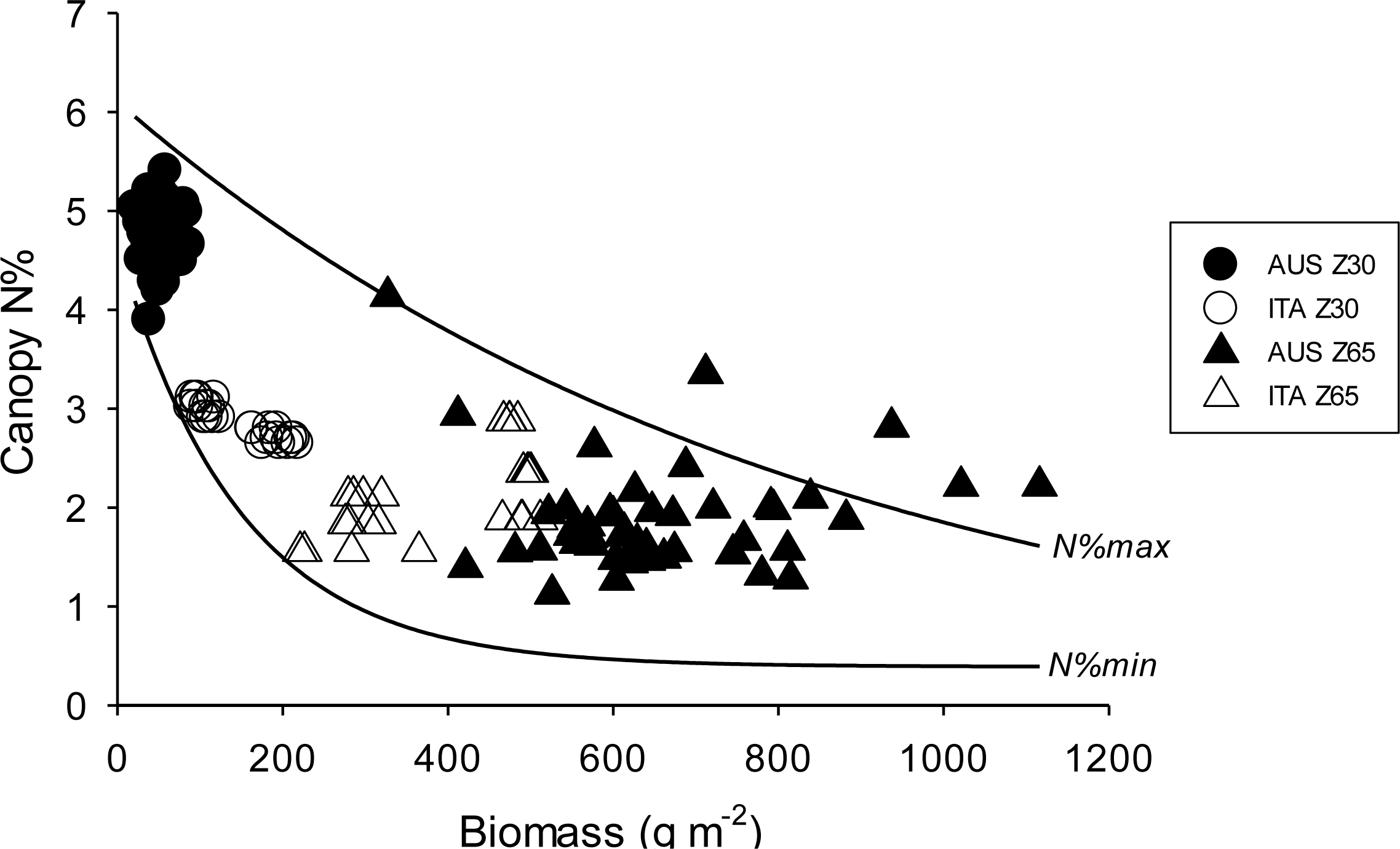
  49. Justes, E.; Mary, B.; Meynard, J.M.; Thelier-Huche, L. Determination of a critical nitrogen dilution curve for winter wheat crops. Ann. Bot 1994, 74, 397–407. [Google Scholar]
  50. Rodriguez, D.; Fitzgerald, G.J.; Belford, R.; Christensen, L.K. Detection of nitrogen deficiency in wheat from spectral reflectance indices and basic crop eco-physiological concepts. Aust. J. Agric. Res 2006, 57, 781–789. [Google Scholar]
  51. Cammarano, D.; Fitzgerald, G.; Basso, B.; Chen, D.; Grace, P.; O’Leary, G. Remote estimation of chlorophyll on two wheat cultivars in two rainfed environments. Crop Pasture Sci 2011, 62, 269–275. [Google Scholar]
  52. Barnes, E.M.; Clarke, T.R.; Richards, S.E. Coincident Detection of Crop Water Stress, Nitrogen Status and Canopy Density Using Ground Based Multispectral Data. In Proceedings of the Fifth International Conference on Precision Agriculture, Madison, WI, USA, 16–19 July 2000; Robert, P.C., Rust, R.H., Larson, W.E., Eds.; American Society of Agronomy (CD-ROM): Madison, WI, USA, 2000. [Google Scholar]
  53. Fitzgerald, G.J.; Rodriguez, D.; O’Leary, G. Measuring and predicting canopy nitrogen concentration in wheat using a spectral index—The canopy chlorophyll content index (CCCI). Field Crop Res 2010, 116, 318–324. [Google Scholar]
  54. Li, F.; Mistele, B.; Hu, Y.; Yue, X.; Yue, S.; Miao, Y.; Chen, X.; Cui, Z.; Meng, Q.; Schmidhalter, U. Remotely estimating aerial n status of phenologically differing winter wheat cultivars grown in contrasting climatic and geographic zones in china and germany. Field Crop Res 2012, 138, 21–32. [Google Scholar]
  55. Serrano, L.; Filella, I.; Penuelas, J. Remote sensing of biomass and yield of winter wheat under different nitrogen supplies. Crop Sci 2000, 40, 723–731. [Google Scholar]
  56. Demetriades-Shah, T.H.; Steven, M.D.; Clark, J.C. High resolution derivative spectra in remote sensing. Remote Sens. Environ 1990, 33, 55–64. [Google Scholar]
  57. Gastal, F.; Lemaire, G. N uptake and distribution in crops: An agronomical and ecophysiological perspective. J. Exp. Bot 2002, 53, 789–799. [Google Scholar]
  58. Lemaire, G.; Jeuffroy, M.H.; Gastal, F. Diagnosis tool for plant and crop N status in vegetative stage. Theory and practices for crop N management. Eur. J. Agron 2008, 28, 614–624. [Google Scholar]
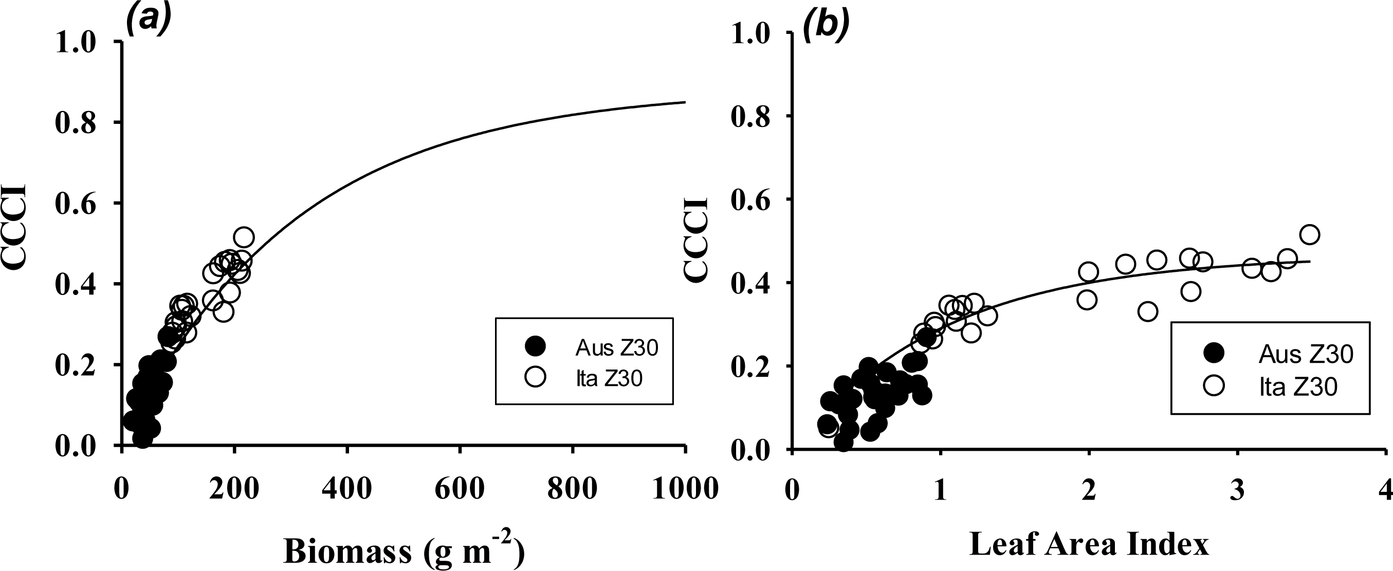
Figure 1. The relationship between canopy nitrogen (N) concentration (%) and biomass (g·m−2) for Australia and Italy at the pseudo-stem elongation (Z30) and anthesis (Z65) stages. The N%max and N%min were calculated following the approach of [50]. AUS, Australia; ITA, Italy.
Remotesensing 06 02827f1
Figure 2. Canopy N (g·N·m−2) measured and predicted with the Canopy Chlorophyll Content Index (CCCI) for the Australian (full symbols) and Italian (open symbols) site at Z30 using the cross-validation method. The line represent the 1:1 relationship.
Remotesensing 06 02827f2
Figure 3. Relationship between the Canopy Chlorophyll Content Index (CCCI) and (a) the leaf area index (LAI), and (b) biomass for the Australian (closed symbols) and Italian (open symbols) site at Z30.
Remotesensing 06 02827f3
Table 1. Vegetation indices used in this study. NDRE, Normalized Difference Red Edge; LAI, Leaf Area Index; NIR, near-infrared.
IndexFormulaReferenceScaleTarget variable
CCCI (Canopy Chlorophyll Content Index) i ( NDRE NDRE min ) ( NDRE max NDRE min )[16]CanopyN Status/Chlorophyll
HS (Hansen and Schjoerring) ( R 573 R 440 ) ( R 573 + R 440 )[26]CanopyBiomass/LAI/N/Chlorophyll
GI (Green Index) R 554 R 677[27]CanopyChlorophyll
BS (Blackburn and Steel) R 652 R 623[28]CanopyPigments/Biophysical Variables
EVI (Enhanced Vegetation Index) 2.5 × ( NIR Red ) ( NIR + C 1 × Re d C 2 × Blue + L )
( C 1 = 6 ; C 2 = 7.5 ; L = 1 )
[29]Canopy/RegionalBiomass/Vegetation Cover
EVI 2 (Enhanced Vegetation Index 2) G × NIR Red NIR + ( 6 7.5 c ) × Red + 1
Red = c × Blue G = f ( c )
[30]Canopy/RegionalBiomass/Vegetation Cover
VARIgreen (Visible Atmospherically Resistant Index) ( Green Red ) ( Green + Red + Blue )[31]Canopy/RegionalVegetation Fraction/LAI
MTVI 1 (Modified Triangular Vegetation Index 1) 1.2 × ( 1.2 × ( R 800 R 550 ) 2.5 × ( R 670 R 550 )[32]CanopyChlorophyll
CARI (Chlorophyll Absorption Reflectance Index) | ( a × R 670 + R 670 + b ) | ( a 2 + 1 ) × R 700 R 670[33]CanopyChlorophyll
TCARI (Transformed CARI) 3 × ( ( R 700 R 670 ) 0.2 × ( R 700 R 550 ) × ( R 700 / R 670 ) )[34]CanopyChlorophyll/LAI/Soil Reflectance
WDVI (Weighted Difference Vegetation Index) NIR a ii × Red[35]CanopyLAI/Biophysical Variables
PVI (Perpendicular Vegetation Index) PVI = NIR ( a 1 × Red ) a 0 ( 1 + a 1 2 )[36]CanopyBiophysical Variables
MSAVI (Modified Soil-Adjusted Vegetation Index) ( 1 + L iv ) × ( R 800 R 670 ) ( R 800 + R 670 + L )[37]CanopyBiophysical Variables
TCI (Triangular Chlorophyll Index) ( 1.2 × ( R 700 R 550 ) 1.5 × ( R 670 R 550 ) × ( R 700 R 670 ) )[32]Leaf/CanopyChlorophyll
RARSb (Ratio Analysis of Reflectance Spectra) R 675 ( R 650 × R 700 )[38]LeafChlorophyll/Pigments
MCARI (Modified CARI) ( ( R 700 R 670 ) 0.2 × ( R 700 R 550 ) ) × R 700 R 670[39]Leaf/CanopyChlorophyll/LAI/Soil reflectance
GR (Green Ratio) R 550 R 670[40]Leaf/CanopyBiomass/Nitrogen
1 DL_DGVI (First Oder Derivative of the Green Vegetation Index using local baseline) λ l λ n | ρ v ( λ vi i ) ρ ( λ i ) | Δ λ vii i[41]Leaf/CanopyLAI/Green Cover
1 DZ_DGVI (First Oder Derivative of the Green Vegetation Index using zero baseline) λ l λ n | ρ ' ( λ i ) | Δ λ i[41]Leaf/CanopyLAI/Green Cover
GIT 1(Gitelson 1) 1 R 700[42]LeafChlorophyll
GIT 2(Gitelson 2) ( Green Blue ) 1 ( NIR Blue ) 1[43]LeafChlorophyll
GIT 3(Gitelson 3) ( ( NIR Blue ) ( Green Blue ) ) 1[43]LeafChlorophyll
Datt 1 R 850 R 710[44]LeafPigments/Chlorophyll
Datt 2 R 860 R 708 × R 550[44]LeafPigments/Chlorophyll
Datt 3 R 672 ( R 550 × R 708 )[44]LeafPigments/Chlorophyll
iCCCI is calculated from the following parameters: NDRE = (790 nm – 720 nm)/(790 nm + 720 nm), NDREmax = 0.61, NDREmin = 0.24 [19];
ii and iiia and b are soil-line coefficients derived from the following equation: NIRsoil = a * REDsoil + b; NIR reflectance was centered at 800 nm, red reflectance at 630 nm and blue reflectance at 450 nm;
ivL is a self-adjustment factor derived from the following equation: L= 1 – 2 × a × NDVI × WDVI;
vthe first derivative of the reflectance;
vithe wavelength;
viithe bandwidth.
Table 2. Mean wheat biophysical variables from Foggia (Italy) for the 2006/2007 growing season at stages Z30 and Z65 for cultivar “Ofanto”.
TreatmentZadoks Growth StageBiomassLAICrop NCrop N

(g·m−2)(m2·m−2)(%)(g·m−2)
0 NZ30104.5 a (3.14) b1.1 a (0.04) b3.0 (0.24)3.1 (0.10)
0 NZ65287.0 (11.20)1.7 (0.11)1.8 (0.07)5.3 (0.30)
90 NZ30191.2 (5.41)2.7 (0.17)2.7 (0.02)5.2 (0.13)
90 NZ65487.0 (4.00)3.1 (0.14)2.3 (0.12)11.5 (0.50)
atreatment means;
bstandard error of the mean (n = 6).
Table 3. Mean wheat biophysical variables from Horsham (Australia) for the 2007 growing season at stages Z30 and Z65 for the cultivar “Yitpi”.
TreatmentZadoks Growth StageBiomassLAICrop NCrop N

(g·m−2)(m2·m−2)(%)(g·m−2)
No CO2 Irrigation 0 NZ3050.2 a (8.34) b0.6 (0.13)5.0 (0.05)2.5 (0.43)
No CO2 Irrigation 0 NZ65573.0 a (49.34) b1.7 (0.04)1.6 (0.27)9.4 (1.45)
No CO2 Irrigation + NZ3045.5 (10.90)0.5 (0.13)5.1 (0.06)2.3 (0.53)
No CO2 Irrigation + NZ65721.0 (56.56)2.1 (0.08)1.9 (0.09)13.7 (1.5)
CO2 Irrigation 0 NZ3049.5 (5.54)0.5 (0.087)2.3 (0.33)4.6 (0.18)
CO2 Irrigation 0 NZ65781.0 (49.42)1.8 (0.11)1.7 (0.15)13.1 (1.30)
CO2 Irrigation + NZ3053.5 (5.95)0.6 (0.097)4.7 (0.11)2.5 (0.33)
CO2 Irrigation + NZ65823.0 (61.04)2.4 (0.49)1.9 (0.15)15.3 (2.60)
CO2 No Irrigation 0 NZ3051.7 (5.51)0.5 (0.068)4.4 (0.21)2.3 (0.32)
CO2 No Irrigation 0 NZ65602.2 (18.44)1.1 (0.14)1.6 (0.08)9.7 (0.33)
CO2 No Irrigation + NZ3058.5 (8.74)0.6 (0.089)4.8 (0.10)2.8 (0.46)
CO2 No Irrigation + NZ65759.5 (119.10)1.3 (0.31)1.7 (0.18)13.4 (3.70)
No CO2 No Irrigation 0 NZ3056.2 (10.00)0.6 (0.10)4.9 (0.10)2.8 (0.51)
No CO2 No Irrigation 0 NZ65631.5 (110.80)1.4 (0.27)2.2 (0.38)14.2 (4.11)
No CO2 No Irrigation + NZ3053.0 (5.00)0.6 (0.075)5.1 (0.13)2.7 (0.30)
No CO2 No Irrigation + NZ65566.2 (12.40)1.1 (0.10)2.1 (0.19)11.7 (1.20)
atreatment means;
bthe standard error of the mean (n = 4).
Table 4. Calibration and validation of the estimation of plant N concentration (%) by vegetation indices for the pooled Australian and Italian site (AUS + ITA) at Z30. Regressions were significant at p < 0.001. Indices are ordered by the coefficient of determination of the cross-validation (CV r2).
Index Name

CalibrationCross-validation

r2 aSE bb cCV r2 dMS e
Indices Developed at the Canopy Level

PVI0.810.4225.10.800.17
VARIgreen0.780.44−4.90.780.20
CARI0.730.49−14.70.720.24
CCCI0.710.51−6.30.700.26
TCARI0.70.52−20.90.690.28
HS0.680.53−16.80.650.29
BS0.500.6613.80.480.45
GI0.490.67−1.90.470.46
MTVI 10.480.68−5.50.420.48
MSAVI0.420.72−180.400.52
EVI0.390.74−5.10.350.56
WDVI0.380.74−9.00.320.56
EVI 20.350.76−5.50.320.59

Indices Developed at the Leaf Level

TCI0.670.54−25.30.660.30
RARSb0.670.540.40.660.30
DATT 20.630.57−170.640.33
MCARI0.630.57−23.70.590.34
GIT 10.590.60.360.580.37
DATT 30.580.610.30.550.39
1 DL_DGVI0.470.68−8.40.430.48
1 DZ_DGVI0.430.71−9.00.390.52
GIT 30.500.66−26.6−0.060.91
GIT 20.730.490.1−0.130.92
DATT 10.360.753.7−0.050.92
aCoefficient of determination of the regression;
bstandard error (%) of the regression;
cslope of the regression line;
dcoefficient of determination from the evaluation obtained through cross-validation (CV);
eestimate of the prediction error (MS).
Table 5. Calibration and validation of the estimation of plant N content (g·m−2) by vegetation indices for the pooled Australian and Italian site (AUS + ITA) at Z30. Regressions were significant at p < 0.001. Indices are ordered by the coefficient of determination of the cross validation (CV r2).
Index Name

CalibrationCross-validation

r2 as.e. bb cCV r2 dMS e
Indices Developed at Canopy Level

CCCI0.730.67.80.720.37
GI0.630.712.60.620.51
VARIgreen0.610.725.30.60.53
EVI0.60.737.80.570.54
MSAVI0.610.7226.50.580.54
EVI 20.60.738.70.560.55
WDVI0.590.7413.80.530.56
MTVI 10.590.747.60.560.59
PVI0.570.76−26.10.540.6
BS0.560.77−17.90.520.63
HS0.480.8417.40.440.73
TCARI0.460.85210.390.74
CARI0.290.9711.60.250.98

Indices Developed at Leaf Level

GR0.630.72.60.620.51
1 DL_DGVI0.590.7411.50.540.57
DATT 20.580.75200.560.58
1 DZ_DGVI0.590.7412.90.530.59
DATT 30.570.76−0.40.510.59
TCI0.480.8426.40.450.76
MCARI0.470.8425.30.440.78
GIT 20.480.84−0.10.310.86
DATT 10.580.75−5.80.161.06
GIT 30.081.11−0.20.151.08
RARSb0.151.07−0.20.111.16
GIT 10.081.1−0.20.051.27
aCoefficient of determination of the regression;
bStandard Error (%) of the regression;
cSlope of the regression line;
dCoefficient of determination from evaluation obtained through cross-validation (CV);
eEstimate of the prediction error (mean square (MS)).

