Vegetation Greenness in Northeastern Brazil and Its Relation to ENSO Warm Events

Abstract

The spatio-temporal variability of trends in vegetation greenness in dryland areas is a well-documented phenomenon in remote sensing studies at global to regional scales. The underlying causes differ, however, and are often not well understood. Here, we analyzed the trends in vegetation greenness for a semi-arid area in northeastern Brazil (NEB) and examined the relationships between those dynamics and climate anomalies, namely the El Nino Southern Oscillation (ENSO) for the period 1982 to 2010, based on annual Normalized Difference Vegetation Index (NDVI) values from the latest version of the Global Inventory Modeling and Mapping Studies (GIMMS) NDVI dataset (NDVI3g) dataset. Against the ample assumption of ecological and socio-economic research, the results of our inter-annual trend analysis of NDVI and precipitation indicate large areas of significant greening in the observation period. The spatial extent and strength of greening is a function of the prevalent land-cover type or biome in the study area. The regression analysis of ENSO indicators and NDVI anomalies reveals a close relation of ENSO warm events and periods of reduced vegetation greenness, with a temporal lag of 12 months. The spatial patterns of this relation vary in space and time. Thus, not every ENSO warm event is reflected in negative NDVI anomalies. Xeric shrublands (Caatinga) are more sensitive to ENSO teleconnections than other biomes in the study area.

1. Introduction

Northeastern Brazil (NEB) is characterized by a semi-arid climate, high intra-annual and inter-annual variability of rainfall and, hence, vegetation productivity [1–4]. The entire region is at risk of desertification processes and loss of biodiversity, due to extensive land conversion for agricultural production and grazing [5,6]. There is high uncertainty about future biome distribution and climate projections [7–9]. Yet, changes in climate, particularly in precipitation dynamics, will lead to changes in the vegetation distribution in the region. So far, little is known about past and recent spatio-temporal dimensions and drivers of variability and trends in vegetation productivity for this area.

Earth observation (EO) satellite data have offered a great potential to monitor land surface conditions, land-cover and land-use conversion and modification at global to regional scales for the last few decades. Many recent publications emphasize vegetation productivity mapping in arid and semi-arid regions worldwide and reveal diverse patterns of decline and increase in vegetation productivity [10–12]. Against the widespread assumption from fieldwork and modelling, several of these studies explicitly reported a “greening” of semi-arid regions worldwide [13,14] and with a focus on the Sahel [15,16]. Using Normalized Difference Vegetation Index (NDVI) time series, Barbosa et al. [1] and Schucknecht et al. [2] reported significant variability in vegetation greenness, particularly for the semi-arid northeastern part of Brazil. The NDVI, computed from time series of medium- to coarse-resolution satellite data, is widely accepted as a proxy for vegetation greenness [17,18]. It thus provides a gross measure of vegetation productivity despite recently discovered restrictions, due to species composition and seasonal cycles [19]. Vegetation greenness in semi-arid regions is causally linked to precipitation occurrence and temporal variation.

In NEB, this seasonal cycle is characterized by a pronounced dry season during the northern summer [20]. This NEB dry season is frequently evolving into an extended period of precipitation deficiency, resulting in droughts that have significant social, economic and environmental impacts. These droughts are assumed to be the consequence of climate anomalies, possibly caused by various teleconnections. Several studies confirmed significant correlations between sea surface temperature (SST) anomalies in the Southern and Central Atlantic, El Nino Southern Oscillation (ENSO) warm events (El Nino), as well as North Atlantic Oscillation (NAO) anomalies and climate extremes in NEB [4,21]. Hastenrath [20] found a significant negative correlation between SST at the coast of Ecuador/Peru and precipitation in NEB. However, Kane [22] argued that the significance of the temporal adjacency of SST anomalies and precipitation extremes in NEB is not strong enough to provide a base for future forecasts. It has nevertheless been recognized that some of the heaviest droughts in NEB coincided with major recent ENSO events [4,22,23], yet none of these studies explicitly investigated the impact of this teleconnection on long- and short-term variability of vegetation greenness/NDVI in the spatial domain.

In this study, we use a 29-year Normalized Difference Vegetation Index (NDVI) time series (1982 to 2010) from the Advanced Very High Resolution Radiometer (AVHRR) on-board the U.S. National Oceanic and Atmospheric Administration (NOAA) satellite to monitor vegetation productivity. The manuscript aims at identifying the dominant inter-annual trends in vegetation greenness in NEB. We address the question of whether land degradation (browning) or rather greening can be observed for the period 1982 to 2010 and further investigate if such vegetation trends can be explained by long-term climate trends. Next to the long-term component, this study also addresses short-term variability in vegetation greenness and its interaction with ENSO warm phases within the study area. Here, particular emphasis lies on the delineation of the spatial extent, temporal dimension (lag) and direction of the teleconnection between ENSO warm phases in the equatorial Pacific and vegetation anomalies for NEB, based on SST anomalies in the Nino 3.4 region of the equatorial Pacific (Nino 3.4 SST; see e.g., [24]) and NDVI anomalies.

2. Methods

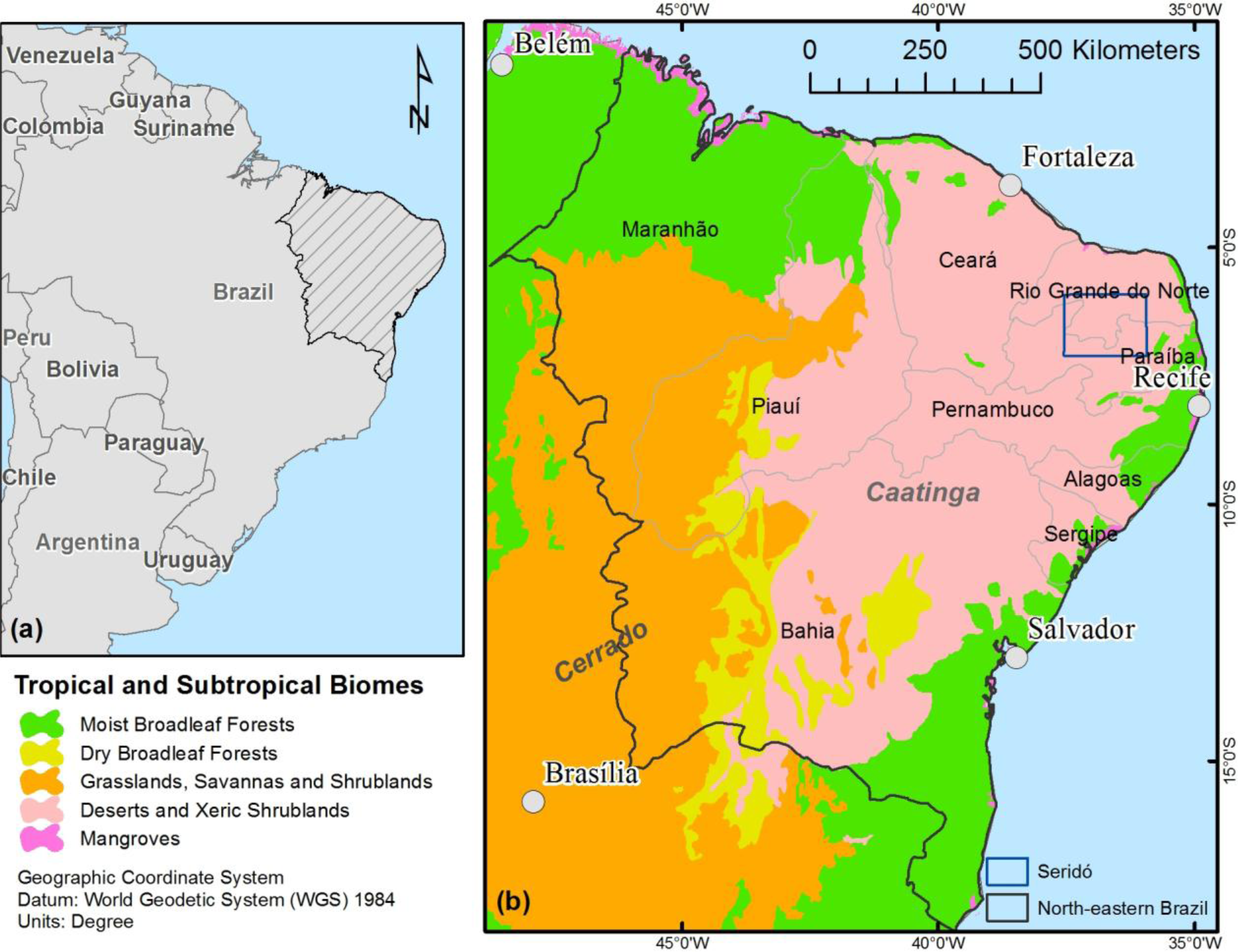
2.1. Study Area: Northeastern Brazil (NEB)

NEB is located in the equatorial zone of South America, ranging from ∼34° to 49° west of Greenwich and from ∼1° to 19° south of the Equator. The region consists of nine federal states, covering an area of about 1,169,000 km² (see the blue rectangle in Figure 1). NEB is delimited by the Atlantic Ocean to the east and northeast, while to the west and southwest, it borders the tropical Amazon rainforest and the South American mainland. In 2007, the region was inhabited by 53 million people [25]. The landscape pattern of NEB is quite heterogeneous and can be divided into three major biomes: (1) the xeric shrublands in the central parts of NEB (Caatinga); (2) the savannas (Cerrado) in western NEB; and (3) the moist broadleaved forests in the coastal regions (Mata Atlantica or Atlantic Forest). Further to the northwest, the region passes into the evergreen moist forests. Mean annual rainfall ranges from less than 400 mm (Caatinga) to more than 1,500 mm (Atlantic Forest). Rainfall in general shows a strong seasonal cycle, with most of the rainfall occurring between February and May [1,3].

The climate of NEB is affected by several large-scale climate systems, the most important one being the Inner-tropical Convergence Zone (ITCZ). In the northern summer time, the ITCZ moves towards the Tropic of Cancer and in winter towards the Tropic of Capricorn, resulting in a pronounced seasonal climate with a dry season during the northern summer. The rainy season in NEB is always related to the southward shift of the ITCZ [21].

Extreme climate conditions, such as prolonged droughts due to climatic anomalies, are associated with an eastward shift of the Walker circulation and, at the same time, with a warming of the middle and upper troposphere, due to increasing SST in the Eastern Pacific [26]. Both processes lead to a temperature increase in the troposphere east of the Andes. In normal periods, the downward branch of the Walker circulation is located over the Eastern Pacific (ENSO normal phase). In ENSO warm phases (El Nino), it is moved eastwards as far as to NEB, resulting in a descending dry air mass. At the same time, the subtropical anticyclones on both sides of the ITCZ are strengthened [26].

The hinterland of the two states, Rio Grande do Norte (RN) and Paraiba (PB), is chosen as a focus region in this study to explicitly investigate vegetation trends and drivers of vegetation variability. In [6], it is described as a nucleus of desertification within NEB (see the blue rectangle in Figure 1).

2.2. Data and Pre-Processing

NDVI time series data were taken from the latest version of the Global Inventory Modeling and Mapping Studies (GIMMS) NDVI dataset (NDVI3g) that has recently been updated for the period of July 1981 to December, 2011 [28,29]. The GIMMS NDVI3g product is derived from imagery obtained from the NOAA AVHRR instrument on-board the NOAA satellite Series 7, 9, 11, 14, 16 and 17. It has been corrected for calibration, view geometry, volcanic aerosols and other effects not related to vegetation change [28]. The dataset consists of bi-monthly maximum value composites (MVC) of NDVI data at a spatial resolution of 8 × 8 km², where the NDVI is calculated as the normalized difference of the spectral reflectance in the red (ρ₁) and near infrared (ρ₂) region of the electromagnetic spectrum or in terms of AVHRR image channels as [30]:

$${\mathit{NDVI}}_{\mathit{AVHRR}}=\raisebox{1ex}{$({\rho }_2-{\rho }_1)$}\!\left/ \!\raisebox{-1ex}{$({\rho }_2+{\rho }_1)$}\right.$$

For the purpose of data integrity with the available climate data, the NDVI3g time series was shortened to the period January 1982 to December 2010, and the bi-monthly data were aggregated to monthly composites using the MVC approach. The pre-processing resulted in a dataset of 348 image channels, each representing the NDVI value of one month. This time series builds the basis for the regression analysis of NDVI data with precipitation and SST in the next sections.

At the same time, the bi-monthly time series were aggregated to annual NDVI values, using the annual sum of NDVI as the key indicator for long-term inter-annual trend analysis. The annual sum of NDVI was chosen, because it reflects vegetation greenness throughout the year. All NDVI time series were finally adjusted for seasonality effects by computing anomalies to the long-term mean for both monthly and annual data.

Rainfall data were received from the Global Precipitation Climatology Centre (GPCC). The GPCC Full Data Reanalysis (Version 6.0) monthly land-surface precipitation product is based on 67,200 rain-gauge stations world-wide that feature record durations of 10 years or longer. It contains the monthly totals on a regular grid with a spatial resolution of 0.5° × 0.5°. The aim of GPCC is to provide highly accurate, spatially explicit, long-term precipitation time series [31]. The temporal coverage of the dataset ranges from January 1901 to December 2010.

The precipitation data were spatially adjusted (stacked) to fit the resolution and grid system of the NDVI3g raster dataset. All GPCC data cells were resampled to a spatial resolution of 8 × 8 km², using a nearest neighbor method to avoid the pseudo accuracy of the spatially enhanced dataset. Monthly precipitation data were summed to annual values and de-seasoned, similar to the NDVI3g series.

The quality of the GPCC gridded precipitation values was validated against a compilation of 77 available rain-gauge station data for the reference period of 1961 to 1990. These stations were located in the two states of Paraiba and Pernambuco and mainly collected and processed by Gomes and Azevedo [32]. The mean value of the linear correlation coefficient, r, between the station data and the corresponding grid cell values is 0.88.

Nino 3.4. SST data were obtained from the Climate Prediction Center (CPC) of NOAA [33]. The values represent the monthly anomalies of SST for the Pacific covering an extent from 5° north to 5° south and 170° to 120° west [34].

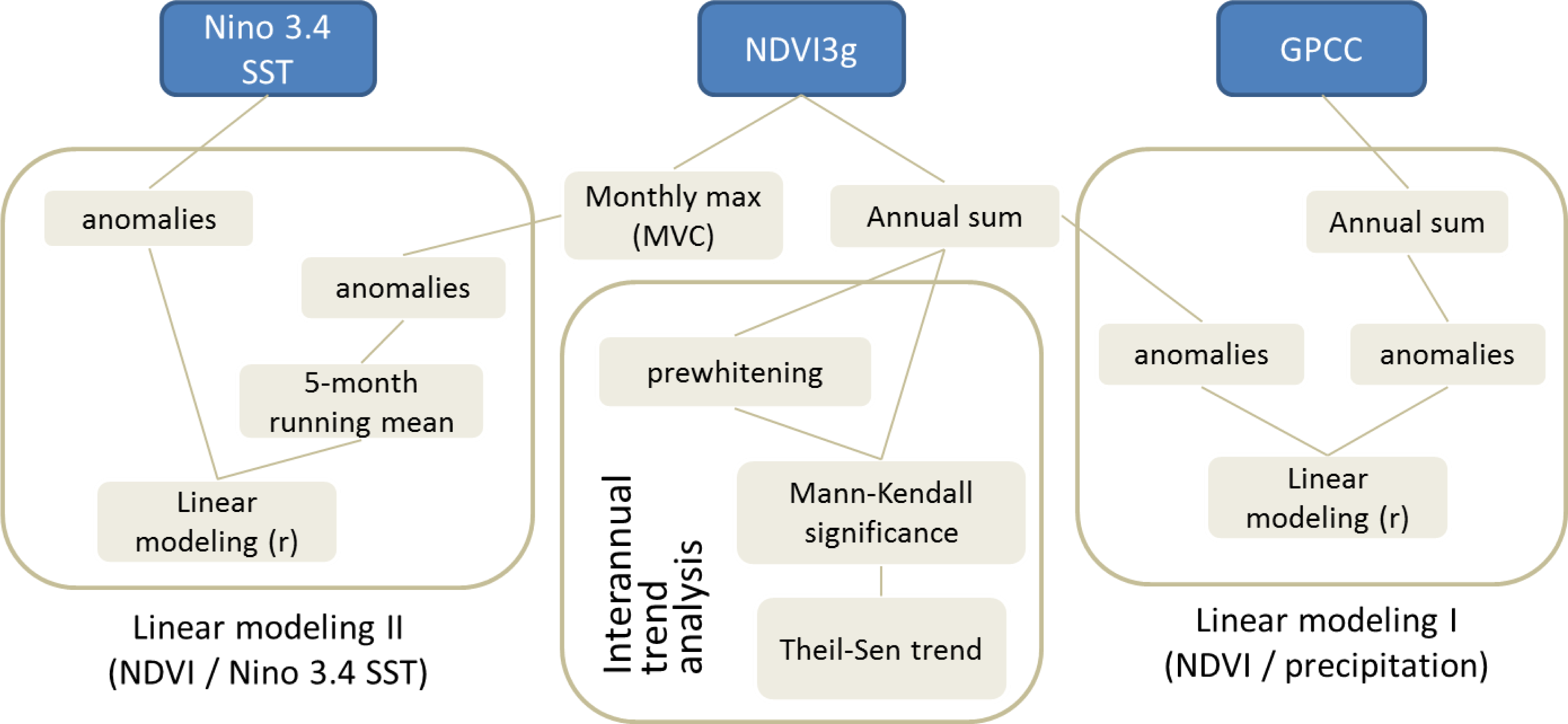
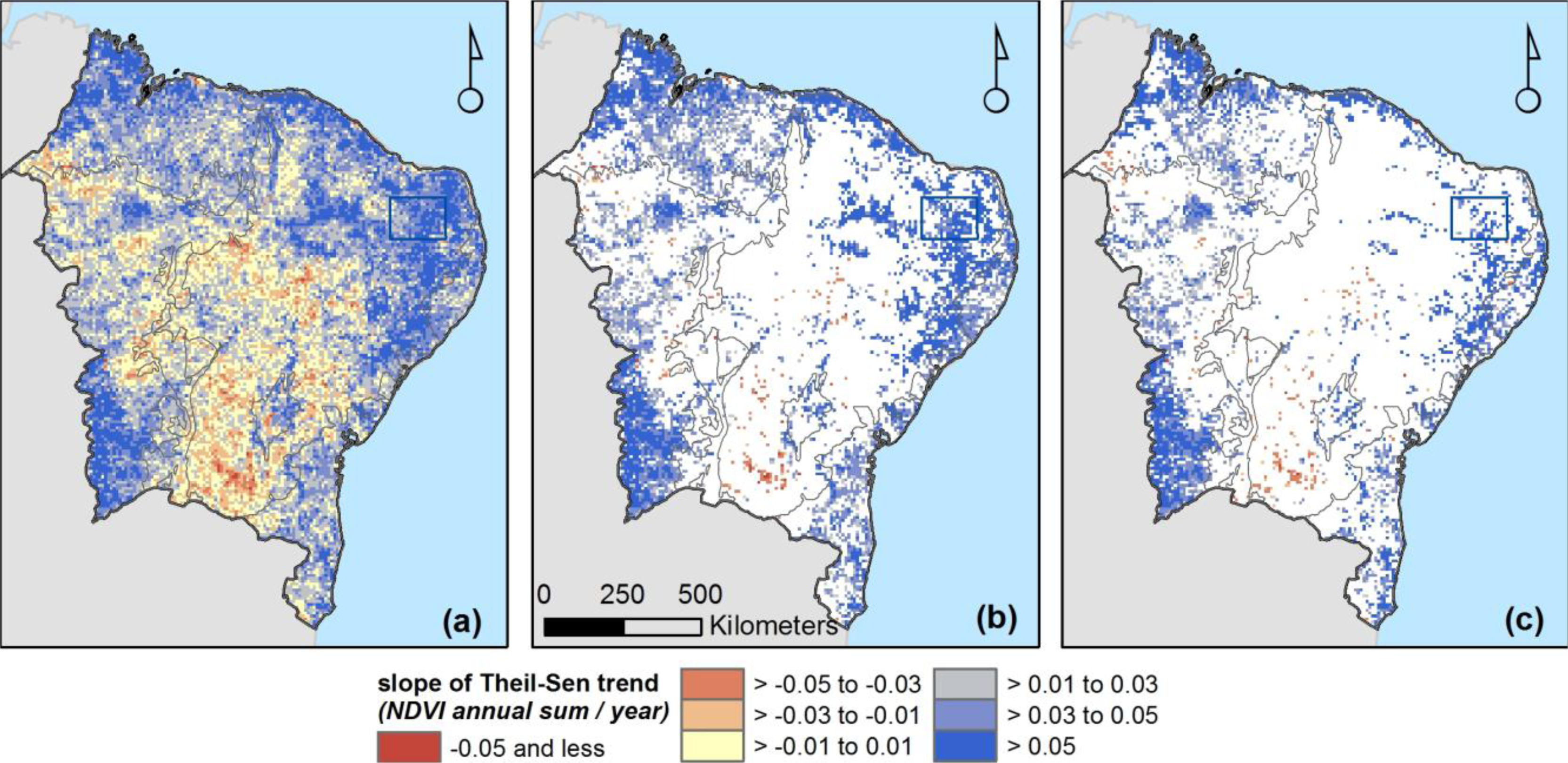
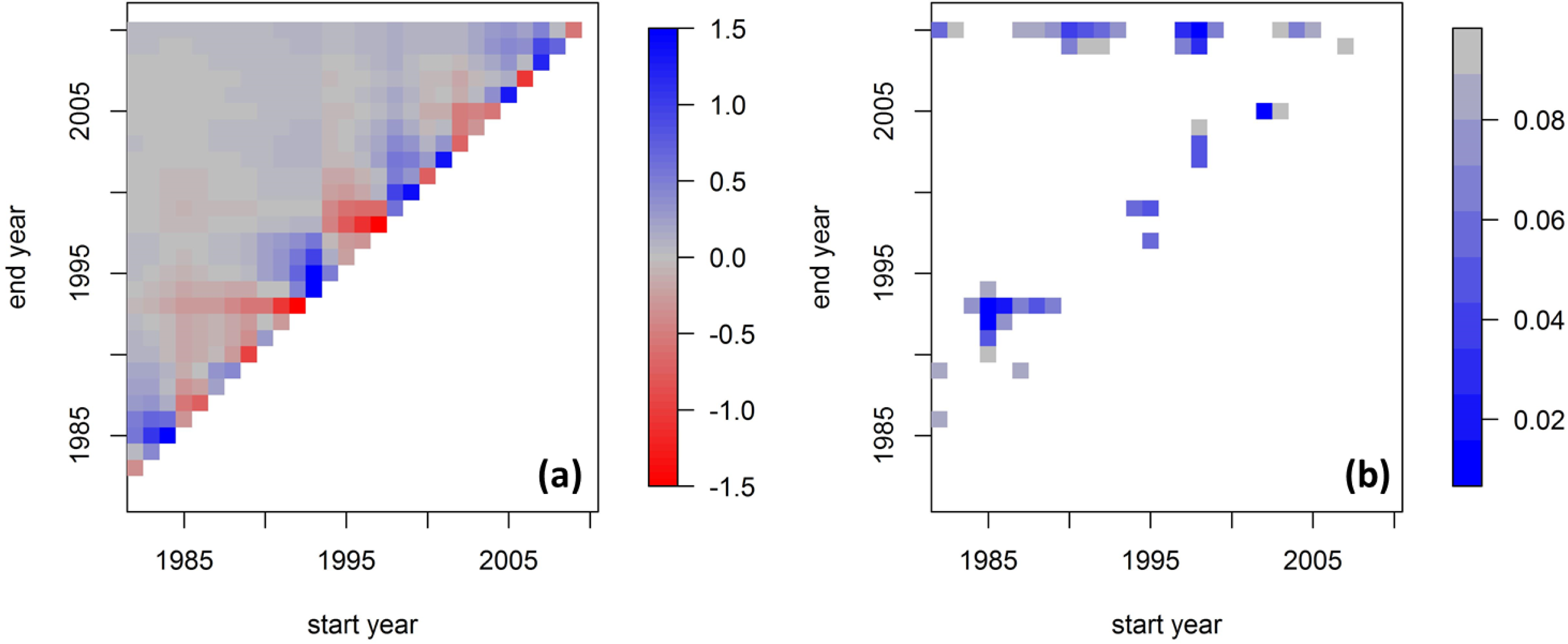
2.3. Inter-Annual Trend Analysis of Annually Summed NDVI3g Data

One of the key indicators to evaluate the existence of alterations in vegetation productivity is the trend in long-term vegetation greenness. Long-term trend analysis in general uses statistical fitting algorithms to measure an increase or decrease of values within time series. Several analyses on the regional to global scales reported that such long-term trends do not automatically behave uniformly in space and time [2,11,13,35]. This is why recent studies tested the trend of changes in vegetation greenness based on spatially explicit proxies, like the NDVI. There are a number of statistical approaches to detect trends in time series and to investigate their direction and strength. The performance of those approaches differs considerable, depending on data quality, spatio-temporal resolution and the applied statistical method itself [35]. An evaluation of all available trend estimators is beyond the scope of this paper and has recently been published by Forkel et al. [36]. The most widely accepted method in environmental sciences to verify the existence of significant long-term trends in time series is the Mann-Kendall test for monotonic trends [37]. This non-parametric test uses ranks instead of the data itself and, thus, is resistant to outliers. It simply compares adjacent data pairs for all values in a time series and calculates a relative frequency of the sum of all intercepts along the time axis. The data range of the test statistic, Z, is [−1;1]. If the value is close to 1, there is a continuous increase in the data; negative values point to a general decrease, and values around 0 indicate no consistent trend. Besides the Z statistic, the test delivers the p-value of the trend statistic, which yields an estimate about the probability that the observed trend could have occurred by chance. It expresses the trend significance. The lower the p-value, the higher is the likelihood that there is a trend in the data. In our work, we used a threshold for the p-value of 0.05 to map exclusively strong significant trends.

A weakness of the Mann-Kendall test is its sensitivity to autocorrelation in time series. Autocorrelation describes how neighboring values in a series depend on each other and how a value in a series explains the preceding value. Yue and Wang [38] discovered that autocorrelation alters the significance of trends in time series, such that high positive autocorrelation increases the Z statistic of the Mann-Kendall trend test. It can be removed using prewhitening techniques, as described by Wang and Swail [39], where the serial correlation is removed in the data residuals, while the trend in the NDVI data is preserved (“trend preserving prewhitening”). However, Bayazit and Onoz [40] pointed out that prewhitening might have a considerable impact on the strength (slope) of the trend. Yue and Wang [38] concluded that the impact of autocorrelation might be neglected for larger time series (n > 50) with a strong trend, and prewhitening might even lead to a masking of existing trends. In the Results section, we compare the results of the trend analysis with and without trend-preserving prewhitening.

The strength estimation of trends in the NDVI time series was based upon the Theil-Sen method. This trend estimator calculates the slope of every single data pair in a time series and uses the median slope to characterize a trend in the data [41]. For long series, the result is often identical to the linear trend. The result is less affected by noise in short series. In NDVI time series, the Theil-Sen trend indicator is easy to use and to interpret, because the slope of the fitted trend line represents the total increase or decrease of NDVI over the given time interval (here: month/year). Thus, it allows a quantification of the rate of change in vegetation greenness for every single pixel.

2.4. Modelling Relations between NDVI3g Time Series and Meteorological Variables

The seasonal and inter-annual development of NDVI as a proxy for vegetation greenness is closely linked to the occurrence and spatio-temporal distribution of precipitation in semi-arid areas. Hence, a significant relation between NDVI and precipitation should turn up as a result of a correlation analysis. Consequently, alterations in the precipitation cycle are assumed to show an impact on vegetation greenness. Based on these two fundamental causal preconditions, the strength of the linear association between annual NDVI and precipitation, as well as between monthly NDVI and Nino 3.4 SST was assessed by calculating the Pearson product moment correlation coefficient (r). The significance of the relations was tested against a threshold of the p-statistic with p = 0.01. Summed annual NDVI and precipitation values enabled the direct comparison of both variables without taking possible lags between them into account. On the other hand, the analysis of monthly values for the NDVI/ENSO relation allowed for a detailed observation of those lags at monthly intervals that provide key information about the existence and spatial inhomogeneity of the ENSO impact in the study area. All relations were tested for the 29-year time series, starting in January, 1982. A summary of the entire processing and analysis workflow is given in Figure 2.

3. Results and Discussion

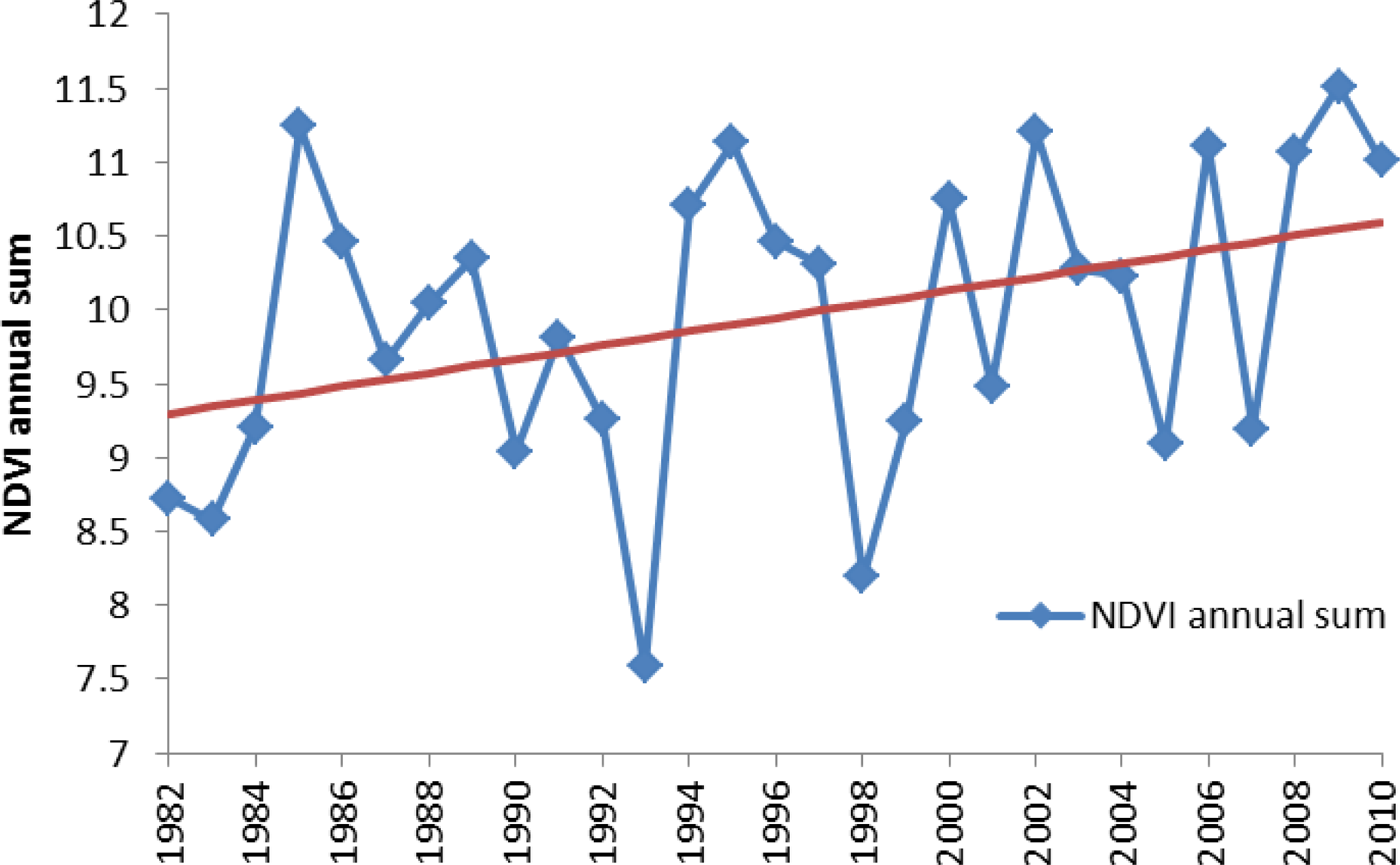
3.1. Trends in Vegetation Greenness

The long-term inter-annual trend analyses of annual summed NDVI values for the period of 1982 to 2010 (Figure 3a) show regions with increasing and decreasing NDVI within the study area. Greening is the dominant process in the northern and northeastern parts, as well as in the southwest, whereas the interior of NEB is characterized by browning, i.e., a decrease in NDVI values. The values of the Theil-Sen slope are given in total units of annually accumulated NDVI change per year and range between −0.15 and +0.24 with a mean slope of 0.0209. However, the 95% confidence interval spreads very tight around the mean from 0.0205 to 0.0213 per year.

Browning is the inferior process, covering only 18% of the area. The remaining 82% show long-term vegetation greening based on the NDVI time series. Considering only significant trends, the overall area, affected by NDVI changes, decreases considerably. Mapping all individual pixels with a significant trend (p < 0.05) yielded an area of 502,848 km² (43% of the study area). Out of this, 95% of the pixels show greening, and only 5% of all significant trends apply to browning and, hence, a decrease in vegetation productivity (Figure 3b).

After prewhitening, the Mann-Kendall test and Theil-Sen slope calculation were carried out again (Figure 3c). The results show that the overall area with significant trends (greening or browning) is considerably reduced from 43% to 31% of the study area after removing temporal auto-correlation. The area affected by significant greening decreases from 478,272 km² to 343,488 km². Irrespective of the applied pre-processing, greening is the dominating trend observed from NDVI time series in the study area (95%/93% of pixels with a significant trend).

Comparing the spatial trend pattern (Figure 3a) with the biome map (Figure 1) reveals that the majority of pixels with browning are related to the Caatinga shrublands. Regions of statistically significant greening (Figure 3b,c) mostly correspond to the croplands in the Southwest and to the moist forests in the northwest and along the coast. Further, a greening nucleus is also evident in the northeastern region of the Caatinga biome, which contains the focus region of our study (Serido). The mean values of annually accumulated NDVI values, together with the Theil-Sen slope for all pixels within the focus region of Serido are displayed in Figure 4. The strong positive trend is obvious, and the inter-annual variability of NDVI and, hence, of vegetation greenness is high. Remarkable negative extremes can be found for the years 1993 and 1998. The relative maxima of the graph are weaker yet evident for 1985 and for the mid-1990s.

The impact of length, the start and the end of the time series on the strength of inter-annual trends has been evaluated by modeling the linear trend of all possible combinations of start and end years in the NDVI time series. This has been exemplarily applied to the mean of the annually accumulated NDVI data for all pixels within the Serido (Figure 5). Blue colors indicate positive trends, and the intensity of the color indicates the trend strength. The key result from this graph shows that the Serido generally faced greening, irrespective of the start year of the time series, when the end is set to 2010 (except for the short inter-annual period from 2008 to 2010). When the end year is modified and the start of the series is fixed to the beginning of the time series, then the outcome is identical (except for the period of 1982 to 1983). If only short periods at the beginning or end of the time series are considered, then the trend is much stronger. Within the time series, the trend patterns become more diffuse with clusters of negative trends; particularly for the short-term periods of 1985 to 1995 and 1995 to 2000. Instead, the strongest positive short-term trends are apparent at the beginning and end of the series, as well as between 1990 and 1997. If we only consider significant linear trends (Figure 5b), then the trend patterns are reduced to only a few recent long-term periods ending in 2010. The remaining significant trends only apply to short-term periods with a cluster between 1985 and 1995.

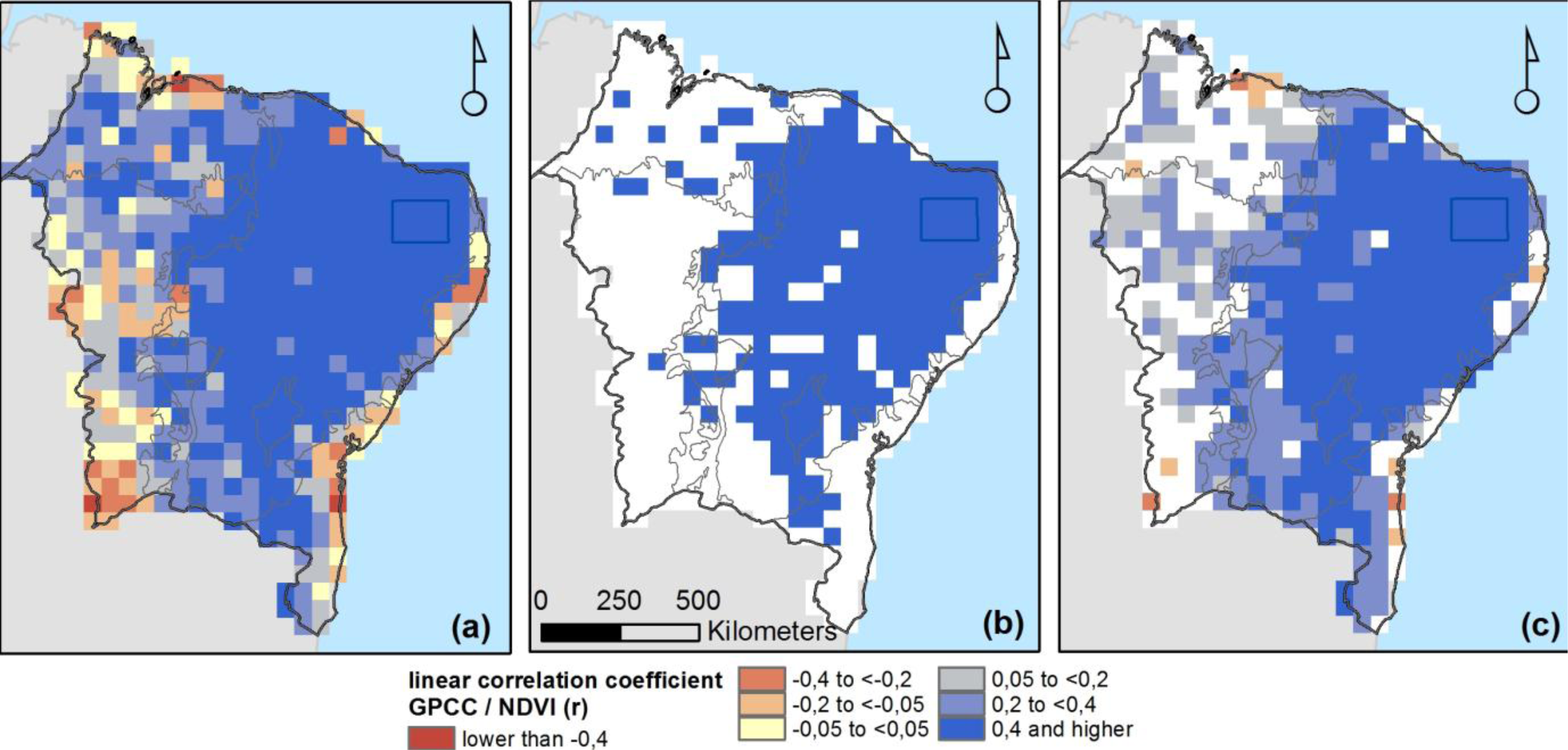
3.2. Relationships between NDVI Trends and Precipitation

The key limiting parameter of vegetation growth in tropical semi-arid regions is precipitation. Consequently, the inter-annual trends in vegetation greenness, as described above, are mainly explained by the availability and spatio-temporal variability of rainfall. To verify this assumption and to obtain a deeper understanding of the NDVI-precipitation relationship in the study area, we computed the linear correlation coefficient, r, at the pixel level for annual, as well as for monthly anomalies of NDVI3g and GPCC precipitation time series from 1982 to 2010. The strength of the relation between these variables is visualized in Figure 6a. Blue pixels symbolize a positive relation between NDVI and precipitation, and red pixels represent negative correlations. Most of the area shows positive correlations between the two variables. Thus, years of higher annual rainfall show a vegetation productivity increase as compared to the long-term mean and vice versa. The regions of significant correlations (Figure 6b) correspond well with the outline of the Caatinga shrublands in Figure 1. The savannas and moist forests show a weaker, mostly non-significant signal on the availability or shortage of annual rainfall. This is confirmed by a stratigraphic analysis of the four biomes prevalent in the study area. The mean coefficients of determination for moist forests (r² = 0.11) and savannas (r² = 0.08) are considerably below the mean values for dry forests (r² = 0.20) and xeric shrublands (r² = 0.36).

The correlation analysis of monthly data uses the NDVI MVC values and monthly summed rainfall data. Opposite of the annual series, the monthly analysis has to account for seasonal effects (phenology) in the NDVI and precipitation signatures. This means that a correlation analysis between the two variables needs to consider the time lag between the beginning of the rainy season and the onset of vegetation greening in semi-arid areas, which is not uniform throughout the season [23]. At the start of the rainy season, the vegetation greening occurs almost simultaneously with the onset of the rainfall. After the rainy season, the maximum in vegetation productivity is reached only two to three months after the rainfall maximum. Accordingly, the vegetation senescence is delayed, too. The highest correlation coefficients for the long-term seasonal analysis were thus observed for a one-month shift between NDVI and GPCC time series, representing the median of the observed lags for all months of the year. The correlation strength is mapped in Figure 6c and shows significant positive relations between NDVI and rainfall for most parts of the study area, especially for the shrubland areas and for substantial parts of the savannas and the moist forests. Negative correlations in the southwest may be associated with the intensive agricultural activities in this region with widely used irrigation techniques.

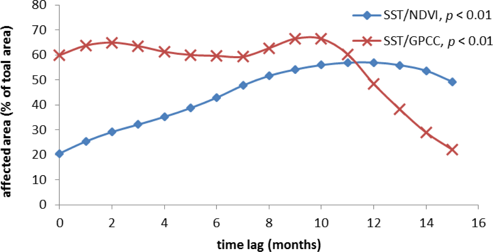
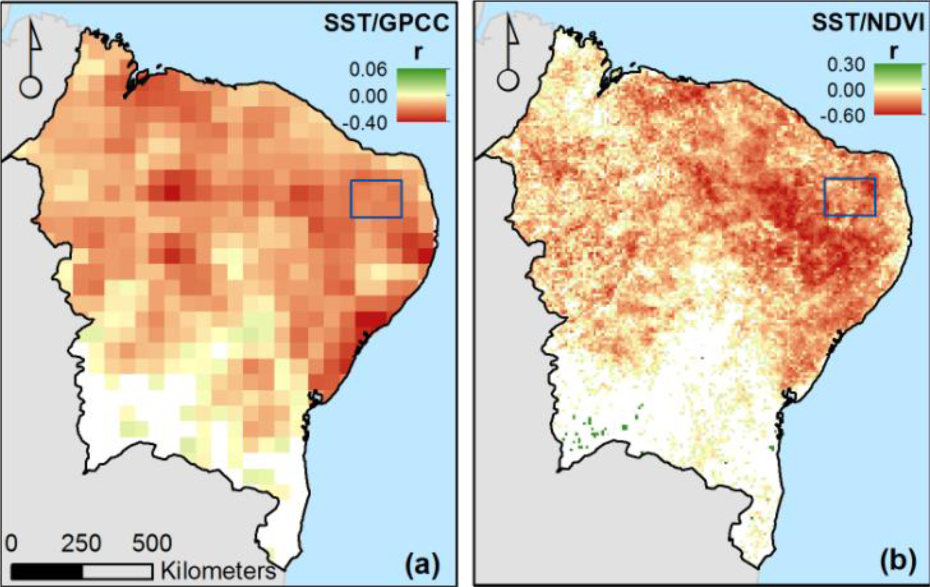
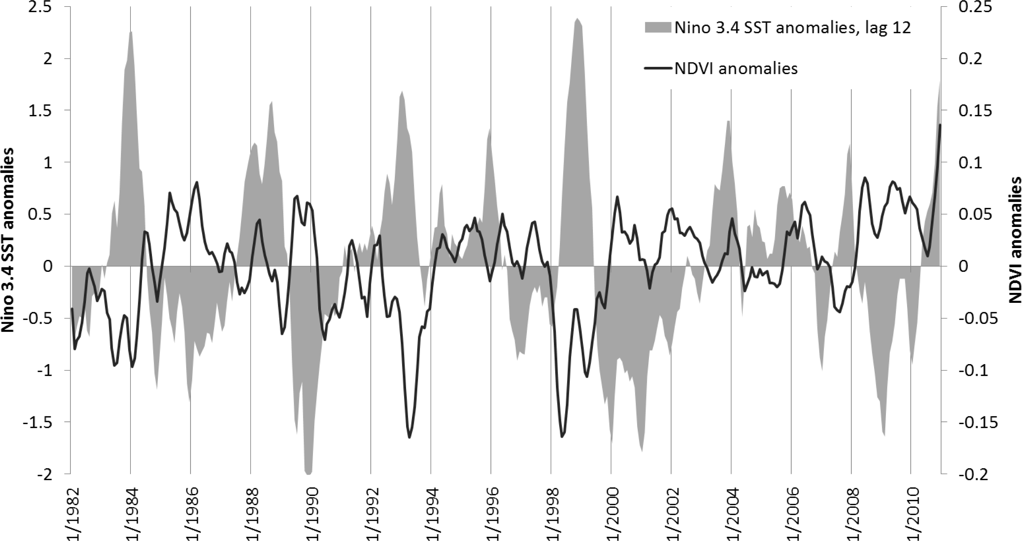
3.3. Impact of El Nino Southern Oscillation Warm Phases on NDVI Trends

The impact of ENSO warm phases on vegetation phenology and droughts in NEB is largely accepted and has been the subject of various climatological studies [4,20,22]. However, the spatial extent, temporal dimension (lag) and direction of the teleconnection between SST in the equatorial Pacific and NDVI for NEB is unknown. The Nino 3.4 SST anomalies comprise a reliable measure of recent ENSO warm phases and were used here as the independent variable for the prediction of NDVI anomalies in monthly time series from 1982 to 2010.

The results of the linear regression analysis between Nino 3.4 SST and NDVI for the complete time period reveal that negative anomalies in monthly NDVI3g data generally follow positive Nino 3.4 SST anomalies with a lag of several months. The spatial extent of the area significantly affected by SST anomalies is a function of the time lag (Figure 7). We investigated monthly lags, ranging from one to 15 months and measured the area where the relation between Nino 3.4 SST anomalies and NDVI3g anomalies is statistically significant at p < 0.01; based on a pixel-wise linear regression of NDVI3g from Nino 3.4 SST for NEB. The maximum affected area is observed for a 12-month lag. The dependency of the time lag between Nino 3.4 SST anomalies and precipitation is weaker. A considerable effect of Nino 3.4 SST anomalies on precipitation is noticeable, even with a lag of a few months only. This effect diminishes rapidly with lags >10 months. The maximum affected area was observed for a temporal lag of nine months. The spatial patterns of the relation between Nino 3.4 SST anomalies and NDVI or precipitation, respectively, are displayed in Figure 8 for the temporal lags indicated above. Both Nino 3.4 SST/NDVI and Nino 3.4 SST/precipitation variation coefficients show a distinct north-south gradient with higher r values in the northern and northwestern parts and weak or no statistical relationships in the southern parts of the region. The Nino 3.4 SST/NDVI plot clearly indicates a nucleus of strong negative correlations in the northeastern part. Areas of high correlation strength can be visibly related to the xeric shrublands (Caatinga). However, due to the latitudinal gradient, the Caatinga is not completely affected by this teleconnection. Weaker correlations are associated with the moist forests of the Mata Atlantica and the evergreen forests in the northwest. Compared with the Caatinga, the savannas and shrublands of the Cerrado are also impacted. Yet, the correlation strength is lower, and the spatial heterogeneity is more complex and shows large areas without any significant correlation in the south of NEB.

The evidence of the temporal lag between Nino 3.4 SST anomalies and NDVI anomalies is further illustrated in the monthly temporal profiles, using the Serido example (Figure 9). In this example, the Nino 3.4 SST graph has been shifted by 12 months, corresponding to the previous analysis of the areas affected by SST anomalies in NEB. The visual interpretation of the graph clearly indicates the negative impact of high positive SST anomalies. The relation is statistically significant with p < 0.01 and r = −0.43 for the period of 1982–2010. A temporal segmentation of the time series in periods of historically documented ENSO warm events in the equatorial Pacific considerably increases the strength of the relationship between the two variables. The highest r values were found for the period of 1983–1986 (r = −0.72) and 1997–2000 (r = −0.67), which cover the respective ENSO warm episodes with a 12-month lag. The graph in Figure 9 also reveals that not all ENSO warm events are followed by a loss in vegetation greenness (e.g., 1986/1987, 2002/2003). On the other hand, only the last ENSO warm event (2002/2003) does not show statistical evidence in the Nino 3.4 SST/NDVI relationship (r = 0.155, p > 0.05).

4. Conclusions

The inter-annual trend analysis of the NDVI3g time series from 1982 to 2010 for NEB reveals a spatial heterogeneity of long-term greening and browning in the study area. Significant trends were observed for 43% of the study area, with the vast majority of trends relating to vegetation greening. This agrees with earlier studies on the same region, using NDVI data from 1982 to 2006 [2]. A direct comparison of the spatial trend patterns revealed a remarkable increase in significant trends (38% from 1982 to 2006) and a clear shift towards greening with more than 90% compared to about 75% in Schucknecht et al. [2]. These differences might be explained by dissimilarities in the length and end time of the NDVI time series and also by modifications in the processing of the NDVI3g time series as compared to the previous GIMMS NDVI data (see, e.g., [29,42]). Another important aspect in comparative studies is the pre-processing of the GIMMS NDVI datasets. In our study, the removal of autocorrelation, using trend-preserving techniques (prewhitening), considerably decreased the strength and spatial extent of significant trends (31% of the total study area as compared to 43% before prewhitening); a consequence of the applied method [40]. It is beyond the scope of this study to argue for a removal of autocorrelation in all NDVI3g-based studies. Our results may highlight the necessity for a better understanding and documentation of pre-processing in NDVI time series trend analysis.

Long-term trend estimators are an appropriate tool to detect monotonic trends. Yet, the occurrence of short-term trends or trend changes within a time series cannot be reproduced from such analysis [43,44]. Jong et al. [45] highlighted the existence and importance of trend changes in long-term analysis. One method to handle this problem is the detection of trend breaks within the time series, as proposed by Verbesselt et al. [43]. Schucknecht et al. [2] adopted that method for an NDVI time series of northeastern Brazil (1982–2006) and showed that the temporal occurrence of trend changes in the area might be related to environmental, as well as climatological triggers. However, the trend break method is susceptible to the start, end and length of the underlying time series data. In our approach, using a slope matrix on an annual basis, we could show the impact of these time series parameters on the slope of the linear trend and, thus, on modeling trend breaks in the time series. The slope matrix proved its usefulness in identifying and analyzing short-term patterns of trend changes in longer time series. It could be demonstrated for the Serido that greening occurs irrespective of the start year of the time series, when the end remains fixed (2010). The strongest positive short-term trends are apparent at the start and end of the series, as well as between 1990 and 1997. Negative short-term trends could be found for the periods of 1985–1995 and 1995–2000.

The climatological drivers of the long- and short-term trend patterns and trend changes of NDVI were investigated with a focus on ENSO-related teleconnections. The general underlying assumption was that strong ENSO warm phases (El Nino) lead to dry conditions in NEB [4,20]. The correlation analysis of NDVI3g data and SST data in the eastern Pacific (Nino 3.4 SST) confirmed this teleconnection and emphasized the importance of the time lag between NDVI decrease in NEB and increasing Nino 3.4 SST anomalies. This is of particular interest in our study area, since the peak of an El Nino event (highest SST anomalies) mostly coincides with the start of the rainy season in semi-arid northeastern Brazil. Thus, the negative impact of a strong El Nino cannot only be observed in the consecutive wet season in NEB, but also in the following season, when vegetation greenness still is reduced significantly. The lag between maximum positive Nino 3.4 SST and negative NDVI3g-anomalies for NEB is about 12 months. This cannot exclusively be interpreted as the temporal delay between the El Nino peak and decrease in precipitation in NEB. It is more adequately explained by the ecological impact of an ENSO warm phase on the regeneration efficiency of the Caatinga shrublands after a serious drought. Another important result of the Nino 3.4 SST-NDVI3g analysis is the detection of related abnormalities. Rodrigues et al. [46], as well as Kane [22] already discussed the influence of El Nino variability on SST anomalies in the equatorial and southern Atlantic and, thus, on climate conditions in NEB. They showed that only strong and long El Nino phases lead to dry conditions in the study area. These results help us to explain the weak or even missing teleconnection for some El Nino phases in NEB that were characterized by long, but weaker El Nino conditions only (e.g., 1986/1987). From the remote sensing perspective, we could also demonstrate that the impact of ENSO warm phases on vegetation greenness in dry periods is not uniform throughout the study area. The spatial patterns of ENSO-related browning are clearly linked to vegetation formations/biomes and, thus, to climate pre-conditions, especially to the seasonal variability of precipitation and, hence, the aridity of the area.

To conclude, the study confirmed the general assumptions about trends in vegetation greenness in semi-arid regions as seen from global Earth observation satellite systems. In line with other remote sensing studies, yet in contrast to many other field studies, we observe vegetation greening based on NDVI time series analysis. Trend changes and anomalies can partly be explained by climatological drivers, such as teleconnections with ENSO warm periods. However, land-use and land-cover change (LULCC) remain key drivers for small-scale degradation in the study area. This may interfere with climatological drivers in future dry periods. Thus, the extent of LULCC and its impact on vegetation and climate in NEB should be further investigated and better understood.

References

1. Barbosa, H.A.; Huete, A.R.; Baethgen, W.E. A 20-year study of NDVI variability over the Northeast Region of Brazil. J. Arid Environ 2006, 67, 288–307. [Google Scholar]
2. Schucknecht, A.; Erasmi, S.; Niemeyer, I.; Matschullat, J. Assessing vegetation variability and trends in north-eastern Brazil using AVHRR and MODIS NDVI time series. Eur. J. Remote Sens 2013, 46, 40–59. [Google Scholar]
3. Nimer, E. Climatologia. do Brasil; Fundacao Instituto Brasileiro de Geografia e Estatistica: Rio de Janeiro, Brazil, 1989. [Google Scholar]
4. Rao, V.B.; Hada, K.; Herdies, D.L. On the severe drought of 1993 in northeast Brazil. Int. J. Climatol 1995, 15, 697–704. [Google Scholar]
5. United Nations Conference on Environment and Development (UNCED). Agenda 21: Programme of Action for Sustainable Development: Rio Declaration on Environment and Development; UNCED: New York, NY, USA, 1992. [Google Scholar]
6. Petta, R.; Ohara, T.; Medeiros, C. Desertification Studies in the Brazilian Northeastern Areas with GIS Database. In Anais XII Simposio Brasileiro de Sensoriamento Remoto, Goiania; Instituto Nacional de Pesquisas Espaciais: São José dos Campos, Brazil, 2005; pp. 1053–1061. [Google Scholar]
7. De Oliveira, G.; Araujo, M.B.; Rangel, T.F.; Alagador, D.; Felizola Diniz-Filho, J.A. Conserving the Brazilian semiarid (Caatinga) biome under climate change. Biodivers. Conserv 2012, 21, 2913–2926. [Google Scholar]
8. Dong, W. The Atlas of Climate Change: Based on SEAP-CMIP5: Super-Ensemble Projection and Attribution (SEAP) of Climate Change; Springer: Heidelberg, Germany, 2013. [Google Scholar]
9. Salazar, L.F.; Nobre, C.A.; Oyama, M.D. Climate change consequences on the biome distribution in tropical South America. Geophys. Res. Lett 2007, 34. 1029/2007GL029695. [Google Scholar]
10. Anyamba, A.; Tucker, C. Analysis of Sahelian vegetation dynamics using NOAA-AVHRR NDVI data from 1981–2003. J. Arid Environ 2005, 63, 596–614. [Google Scholar]
11. De Jong, R.; de Bruin, S.; de Wit, A.; Schaepman, M.E.; Dent, D.L. Analysis of monotonic greening and browning trends from global NDVI time-series. Remote Sens. Environ 2011, 115, 692–702. [Google Scholar] [Green Version]
12. Zhao, M.; Running, S.W. Drought-induced reduction in global terrestrial net primary production from 2000 through 2009. Science 2010, 329, 940–943. [Google Scholar]
13. Fensholt, R.; Langanke, T.; Rasmussen, K.; Reenberg, A.; Prince, S.D.; Tucker, C.; Scholes, R.J.; Le, Q.B.; Bondeau, A.; Eastman, R.; et al. Greenness in semi-arid areas across the globe 1981–2007—An earth observing satellite based analysis of trends and drivers. Remote Sens. Environ 2012, 121, 144–158. [Google Scholar]
14. Hellden, U.; Tottrup, C. Regional desertification: A global synthesis. Glob. Planet. Change 2008, 64, 169–176. [Google Scholar]
15. Dardel, C.; Kergoat, L.; Hiernaux, P.; Mougin, E.; Grippa, M.; Tucker, C. Re-greening Sahel: 30 years of remote sensing data and field observations (Mali, Niger). Remote Sens. Environ 2014, 140, 350–364. [Google Scholar]
16. Herrmann, S.M.; Anyamba, A.; Tucker, C.J. Recent trends in vegetation dynamics in the African Sahel and their relationship to climate. Global Environ. Change 2005, 15, 394–404. [Google Scholar]
17. Myneni, R.B.; Hall, F.G.; Sellers, P.J.; Marshak, A.L. The interpretation of spectral vegetation indices. IEEE Trans. Geosci. Remote Sens 1995, 33, 481–486. [Google Scholar]
18. Bastin, G.N.; Pickup, G.; Pearce, G. Utility of AVHRR data for land degradation assessment: A case study. Int. J. Remote Sens 1995, 16, 651–672. [Google Scholar]
19. Mbow, C.; Fensholt, R.; Rasmussen, K.; Diop, D. Can vegetation productivity be derived from greenness in a semi-arid environment? Evidence from ground-based measurements. J. Arid Environ 2013, 97, 56–65. [Google Scholar]
20. Hastenrath, S. Circulation and teleconnection mechanisms of Northeast Brazil droughts. Prog. Oceanogr 2006, 70, 407–415. [Google Scholar]
21. Haylock, M.R.; Peterson, T.C.; Alves, L.M.; Ambrizzi, T.; Anunciacao, Y.M.; Baez, J.; Barros, V.R.; Berlato, M.A.; Bidegain, M.; Coronel, G.; et al. Trends in total and extreme South American rainfall in 1960–2000 and links with sea surface temperature. J. Climate 2006, 19, 1490–1512. [Google Scholar]
22. Kane, R.P. Prediction of droughts in north-east Brazil: Role of ENSO and use of periodicities. Int. J. Climatol 1997, 17, 655–665. [Google Scholar]
23. Erasmi, S.; Maurer, F.; Petta, R.A.; Gerold, G.; Barbosa, M.P. Inter-annual variability of the normalized difference vegetation index over Northeast Brazil and its relation to rainfall and El Nino Southern Oscillation. Geo. Oko 2009, 30, 185–206. [Google Scholar]
24. Trenberth, K.E. The definition of El Nino. B. Am. Meteorol. Soc 1997, 78, 2771–2777. [Google Scholar]
25. Instituto Brasileiro de Geografia e Estatística (IBGE). Censo. Demografico 2010: Características. da Populacao e dos Domicilios: Resultados do Universo; IBGE: Rio de Janeiro, Brazil, 2011. [Google Scholar]
26. Lau, K.M.; Zhou, J.Y. Anomalies of the South American summer monsoon associated with the 1997–99 El Nino southern oscillation. Int. J. Climatol 2003, 23, 529–539. [Google Scholar]
27. Olson, D.M.; Dinerstein, E.; Wikramanayake, E.D.; Burgess, N.D.; Powell, G.V.; Underwood, E.C.; D’Amico, J.A.; Itoua, I.; Strand, H.E.; Morrison, J.C.; et al. Terrestrial ecoregions of the worlds: A new map of life on Earth. Bioscience 2001, 51, 933–938. [Google Scholar]
28. Tucker, C.; Pinzon, J.; Brown, M.; Slayback, D.; Pak, E.; Mahoney, R.; Vermote, E.; El Saleous, N. An extended AVHRR 8-km NDVI dataset compatible with MODIS and SPOT vegetation NDVI data. Int. J. of Remote Sens 2005, 26, 4485–4498. [Google Scholar]
29. Zhu, Z.; Bi, J.; Pan, Y.; Ganguly, S.; Anav, A.; Xu, L.; Samanta, A.; Piao, S.; Nemani, R.; Myneni, R. Global data sets of Vegetation Leaf Area Index (LAI)3g and Fraction of Photosynthetically Active Radiation (FPAR)3g derived from Global Inventory Modeling and Mapping Studies (GIMMS) Normalized Difference Vegetation Index (NDVI3g) for the period 1981 to 2011. Remote Sens 2013, 5, 927–948. [Google Scholar]
30. Tucker, C.J. Red and photographic infrared linear combinations for monitoring vegetation. Remote Sens. Environ 1979, 8, 127–150. [Google Scholar]
31. Full Data Reanalysis Version 6.0 at 0.5: Monthly Land-Surface Precipitation from Rain-Gauges Built on GTS-Based and Historic Data. Available online: ftp://ftp-anon.dwd.de/pub/data/gpcc/html/fulldata_v6_doi_download.html (accessed on 25 February 2014).
32. Gomes, L.; Azevedo, P. Avaliação do processo de semidesertificação no Estado da Paraíba, Brasil: Trabalho de Conclusão do Curso de Meteorologia; Universidade Federal de Campina Grande: Campina Grande, Brazil, 2008. [Google Scholar]
33. Climate Prediction Center. Monitoring and Data: Current Monthly Atmospheric and Sea Surface Temperatures Index Values; Climate Prediction Center: Maryland, MD, 2012. Available online: http://www.cpc.ncep.noaa.gov/data/indices/ (accessed on 25 February 2014).
34. Trenberth, K.E.; Stepaniak, D.P. Indices of El Nino evolution. J. Climate 2001, 14, 1697–1701. [Google Scholar]
35. Vrieling, A.; de Leeuw, J.; Said, M. Length of growing period over Africa: Variability and trends from 30 years of NDVI time series. Remote Sens 2013, 5, 982–1000. [Google Scholar]
36. Forkel, M.; Carvalhais, N.; Verbesselt, J.; Mahecha, M.; Neigh, C.; Reichstein, M. Trend change detection in NDVI time series: Effects of inter-annual variability and methodology. Remote Sens 2013, 5, 2113–2144. [Google Scholar]
37. Mann, H.B. Nonparametric tests against trend. Econometrica 1945, 13, 245–259. [Google Scholar]
38. Yue, S.; Wang, C.Y. Applicability of prewhitening to eliminate the influence of serial correlation on the Mann-Kendall test. Water Resour. Res 2002, 38. [Google Scholar] [CrossRef]
39. Wang, X.L.; Swail, V.R. Changes of extreme wave heights in Northern Hemisphere oceans and related atmospheric circulation regimes. J. Climate 2001, 14, 2204–2221. [Google Scholar]
40. Bayazit, M.; Onoz, B. To prewhiten or not to prewhiten in trend analysis? Hydrolog. Sci. J 2007, 52, 611–624. [Google Scholar]
41. Sen, P.K. Estimates of the regression coefficient based on Kendall’s tau. J. Am. Stat. Assoc 1968, 63, 1379–1389. [Google Scholar]
42. Jiang, N.; Zhu, W.; Zheng, Z.; Chen, G.; Fan, D. A comparative analysis between GIMSS NDVIg and NDVI3g for monitoring vegetation activity change in the northern hemisphere during 1982–2008. Remote Sens 2013, 5, 4031–4044. [Google Scholar]
43. Verbesselt, J.; Hyndman, R.; Newnham, G.; Culvenor, D. Detecting trend and seasonal changes in satellite image time series. Remote Sens. Environ 2010, 114, 106–115. [Google Scholar]
44. Liu, G.; Liu, H.; Yin, Y. Global patterns of NDVI-indicated vegetation extremes and their sensitivity to climate extremes. Environ. Res. Lett 2013, 8. [Google Scholar] [CrossRef]
45. De Jong, R.; Verbesselt, J.; Schaepman, M.E.; de Bruin, S. Trend changes in global greening and browning: Contribution of short-term trends to longer-term change. Glob. Chang. Biol 2012, 18, 642–655. [Google Scholar]
46. Rodrigues, R.R.; Haarsma, R.J.; Campos, E.J.D.; Ambrizzi, T. The Impacts of Inter-El Nino variability on the tropical Atlantic and Northeast Brazil climate. J. Climate 2011, 24, 3402–3422. [Google Scholar]
Figure 1. (a) Overview of the study area of northeastern Brazil. (b) Tropical and subtropical biomes in northeastern Brazil are after Olson et al. [27], including the outline of the focus region “Serido”.
Remotesensing 06 03041f1
Figure 2. Workflow for the processing of time series from Normalized Difference Vegetation Index (NDVI) 3g (NDVI3g), Global Precipitation Climatology Centre (GPCC) and Nino 3.4 sea surface temperature (SST) data. MVC, maximum value composite.
Remotesensing 06 03041f2
Figure 3. The results of the inter-annual trend-analysis for annually accumulated NDVI3g time series (1982–2010). (a) The slope of the Theil-Sen trend for raw annual NDVI3g data (annual sum); (b) the slope of significant trends in raw annual NDVI3g data (annual sum); (c) the slope of significant trends in annual NDVI3g data after prewhitening (annual sum) (white = no significance, p < 0.05). Grey lines represent the outlines of the biomes from Figure 1.
Remotesensing 06 03041f3
Figure 4. Mean value of annually accumulated NDVI3g data (1982–2010) for all pixels within the focus region of Serido (red line = Theil-Sen trend).
Remotesensing 06 03041f4
Figure 5. Impact of the start and end of NDVI time series (annual sum) on the strength of the trend that is observed in the Serido. (a) The slope of the linear trend (accumulated NDVI/year); (b) the significance of the linear trend (only for p < 0.1).
Remotesensing 06 03041f5
Figure 6. The results of the linear correlation analysis for NDVI3g time series (1982–2010). (a) The correlation coefficient (r) for GPCC and NDVI3g data (annual anomalies); (b) the areas with significant relation between GPCC and NDVI3g data (annual anomalies); (c) significant relationships (lag = +1) between monthly GPCC and NDVI3g data (monthly anomalies); white = no significance (p < 0.01). Grey lines represent the outlines of the biomes from Figure 1.
Remotesensing 06 03041f6
Figure 7. The dependency of total affected area on lag length (in months) for the linear relation between monthly NDVI3g and Nino 3.4 SST data (blue) and monthly GPCC precipitation and Nino 3.4 SST data (red).
Remotesensing 06 03041f7
Figure 8. Coefficient of variation (r) for linear regression for the period of 1982–2010 between monthly Nino 3.4 SST anomalies and (a) GPCC precipitation data (lag = 9) and (b) NDVI3g data (lag = 12); (white = no significance, p < 0.01).
Remotesensing 06 03041f8
Figure 9. The temporal profile of monthly NDVI3g anomalies for the focus region of Serido, compared to monthly Nino 3.4 SST anomalies with a temporal lag of +12 months.
Remotesensing 06 03041f9