Forest Canopy Heights in the Pacific Northwest Based on InSAR Phase Discontinuities across Short Spatial Scales

Abstract

Rapid land use changes are substantially altering the global carbon budget, yet quantifying the impact of these changes, or assessing efforts to mitigate them, remains challenging. Methods for assessing forest carbon range from precise ground surveys to remote-sensing approaches that provide proxies for canopy height and structure. We introduce a method for extracting a proxy for canopy heights from Interferometric Synthetic Aperture Radar (InSAR) data. Our method focuses on short-spatial scale differences between forested and cleared regions, reducing the impact of errors from variations in atmospheric water vapor or satellite orbital positions. We generate time-varying, Landsat-based maps of land use and perform our analysis on the original wrapped (modulo-2π) data to avoid errors introduce by phase unwrapping and to allow assessment of the confidence of our results (within 3–4 m in many cases). We apply our approach to the Pacific Northwest, which contains some of the world’s tallest trees and has experienced extensive clearcutting. We use SAR imagery acquired at L-band by the PALSAR instrument on the Japanese Aerospace Exploration Agency’s (JAXA) Advanced Land Observation Satellite (ALOS). As SAR data archives expand, our approach can complement other remote-sensing methods and allow time-variable assessment of forest carbon budgets worldwide.

1. Introduction

The contribution of ongoing global deforestation to climate change has been of increasing concern over the past few decades (e.g., [1–3]). An estimated 650 billion metric tons of carbon are stored in forests globally, more than is present in the atmosphere [4]. Approximately 12% of anthropogenic greenhouse gas emissions can be attributed to CO₂ emitted as a result of deforestation [5]. Any legislation that seeks to curb deforestation rates must be accompanied by a means for verifying compliance and taking inventories of current forest stocks. Such inventories also allow assessment of the efficacy of forest management practices and monitoring of overall forest health.

Currently, many of the statistics on global forests depend on the self-reporting of nations, making them subject to the ability and desire of a nation to accurately report on its forest inventory [4]. Vegetation structure and canopy height are two parameters of interest when assessing a forest inventory, and can be combined with allometric relationships to determine the biomass and, in turn, carbon stock of a forested region (e.g., [6–9]). These inventories are typically undertaken through comprehensive ground surveys or remote sensing methods that rely on LiDAR (e.g., [10–19]), optical or radar imagery (both the amplitude and interferometric products) (e.g., [11,12,15–17,19–25]). Ground surveys on a local scale are cost-effective and allow for measurements and observations of forest characteristics such as species diversity, overall health, and forest density to be made with relative ease; however, surveys with the desired short repeat times would require a great deal of time and human labor and, for logistical and political reasons, are difficult to perform in many critical forested regions (e.g., [14,26]). In light of these challenges, remote sensing methods that can be conducted at a global scale with frequent repeat intervals can serve as a powerful complement to ground surveys [9].

Numerous studies have investigated the capabilities of Light Detection And Ranging (LiDAR) to determine forest characteristics such as vegetation density, structure, and canopy height (e.g., [16,27–29]). These studies suggest that, under optimal conditions, canopy height within the footprint of the LiDAR beam can be measured with centimeter-scale accuracy, at least in areas where slopes are <5 degrees [18]. A global canopy height map produced using Geoscience Laser Altimeter System (GLAS) data combined with Moderate Resolution Imaging Spectroradiometer (MODIS) data indicates that canopy heights within our study region in the Pacific Northwest (Figure 1) are among the tallest in the world, with many regions containing 35–65 m tall trees [16]. Both satellite- and airplane-based platforms are capable of frequent repeat LiDAR measurements, potentially on global scales. However, the interpretation of LiDAR data is complicated by cloud cover and steep slopes, both of which are frequent conditions in many forested regions of interest (e.g., [14,29–32]).

Satellite-based synthetic aperture radar (SAR) complements the approaches listed above, since active imaging at microwave wavelengths is possible at night (when optical imagery is not available) and in regions with dense cloud cover (which presents challenges for optical imagery and LiDAR systems). SAR systems generate images that are ∼100 km × 100 km in scale with pixels on the order of a few tens of meters or smaller (e.g., [33]). The repeat intervals for SAR satellites range from days to months, potentially allowing for frequent, global repeat observations of forest properties [34]. Previous studies have investigated the feasibility of using the backscattered amplitude from SAR as well as the coherence information from pairs of images as a proxy for biomass and vegetation structure, particularly when data from multiple polarizations is available (e.g., [20–23,27,32,35–39]). Comparisons of bare-earth digital elevation models (DEMs) with the elevation product produced by the Shuttle Radar Topography Mission’s (SRTM) or other SAR platforms have also enabled determination of canopy heights (e.g., [12,15,28]). The use of interferometric phase values themselves, rather than just coherence, has also been explored (e.g., [22,35,36]), particularly for systems where the repeat times are short relative to the timescales of temporal decorrelation (e.g., [33]).

Here, we present an approach that uses the phase information from time series of InSAR data acquired on satellite platforms to constrain tree heights over the Pacific Northwest. We focus on a set of SAR imagery acquired at L-band by the ALOS satellite, which results in high coherence in forests relative to the C-band imagery that dominated the available satellite-based SAR data catalogs before the ALOS mission. We focus on differences in interferometric phase averaged between forested and cleared regions (e.g., [35]) assimilated with satellite-based maps of land cover that allow us to apply the phase differencing over large regions affected by time-varying land use. This method, which does not require simultaneous imaging or polarimetric data, capitalizes on the growing sets of SAR time series and related optical imagery datasets that are available worldwide, providing a proxy for canopy height that differs from the approaches described above.

2. Method: Extracting Tree Heights from Short-Spatial Scale InSAR Phase Variations

Interferometric phase in repeat-track InSAR depends on a combination of the geometry of the satellite or airborne platforms at the time of image acquisition, topographic relief, the reflective properties of the Earth’s surface, and changes in the travel time of radar waves between the ground and the imaging platform (e.g., [33]). The latter can include variations in atmospheric water vapor or the ionosphere, as well as deformation of the ground surface due to processes such as earthquakes, landslides or anthropogenic activities (e.g., [33,40,41]). Because the contribution from radar path delays and errors in our knowledge of satellite locations often dominates interferograms (e.g., [42–44]), particularly at longer spatial scales (>10 s of km), the value of the interferometric phase itself (rather than just the coherence) has so far been of limited utility in forest studies. In this paper, we present an algorithm for determining forest canopy heights that focuses on short-spatial-scale (<few km) interferometric phase variations between adjacent cleared and forested regions in the Pacific Northwest. Most of the error sources for InSAR that result in coherent biases to the phase (e.g., satellite orbital errors, variations in atmospheric water vapor) cancel out over these short distances.

As described above, interferometric phase is affected by many variables, including errors in the digital elevation model (DEM) used to remove the effects of topography (e.g., [45]). Trees present within a particular pixel will act as sources of apparent “DEM error”, since they raise the height of the effective phase scatterers within that pixel above the bare ground surface. Differencing of SAR-based DEMs such as SRTM and “bare-earth” DEMs (available throughout much of the United States) have resulted in maps of canopy height (e.g., [12,15]). The simultaneous acquisition of images that occurred as part of SRTM resulted in negligible contributions from atmospheric noise and temporal decorrelation, whereas SAR acquisitions from typical satellite platforms are separated by days to months.

In the absence of frequent repeats of missions such as SRTM, we present an approach for extracting information about tree heights using many interferograms and focusing on short spatial scales. The magnitude of the topographic effect on interferometric phase depends linearly on the spatial separation between the satellite’s positions at the time of image acquisition (also known as the perpendicular baseline, B_┴, (e.g., [46]). The contribution from all other factors affecting the interferometric phase is expected to be random with respect to B_┴. The difference in phase between a cleared region and the immediately adjacent forest for sets of interferograms with a range of B_┴ has been shown to be directly related to the height of the effective scattering phase center for that group of trees (e.g., [35]). Differencing over such a short spatial scale cancels out errors from atmospheric effects and orbital configurations. There are other significant sources of error, such as temporal decorrelation and changes in the dielectric constant of the surface due to factors such as variations in soil moisture within the cleared areas, but none of those results in a change in phase that correlates positively with baseline.

An example interferogram covering a 46-day time interval is shown in Figure 2a. The coherence is typical for interferograms of this time span, with most of the decorrelation occurring in regions of open water or the higher elevations that sometimes experience snowfall. The signals at large spatial scales (10’s of km) in Figure 2 can be attributed to variations in atmospheric water vapor and/or inaccuracies in our knowledge of the satellite location at the two acquisition times—the phase value at any particular point provides essentially no information about canopy heights. Also apparent are small (∼1 km² area), quasi-rectangular features with an interferometric phase value that differs abruptly from surrounding pixels. We attribute these features to the differences in phase scattering height relative to the bare earth in forested vs. cleared regions. Comparisons with optical imagery verify the relationship to logged regions (Figure 2b,c). As expected, the difference in phase between adjacent cleared and forested regions increases linearly with B_┴ when we examine multiple interferograms covering the same area (Figure 3). This result agrees with previous work from [35] using ERS data (C-band) with repeat passes between 3–12 days. Note that in Figure 3 we have chosen the location of forested and cleared regions by hand for clarity—our automated approach skips this time-consuming step.

Below, we describe the methods we use to estimate heights over large areas (∼100 km). The large-scale application requires the following steps:

(a)

Generation of all interferograms possible from existing SAR imagery catalog.

(b)

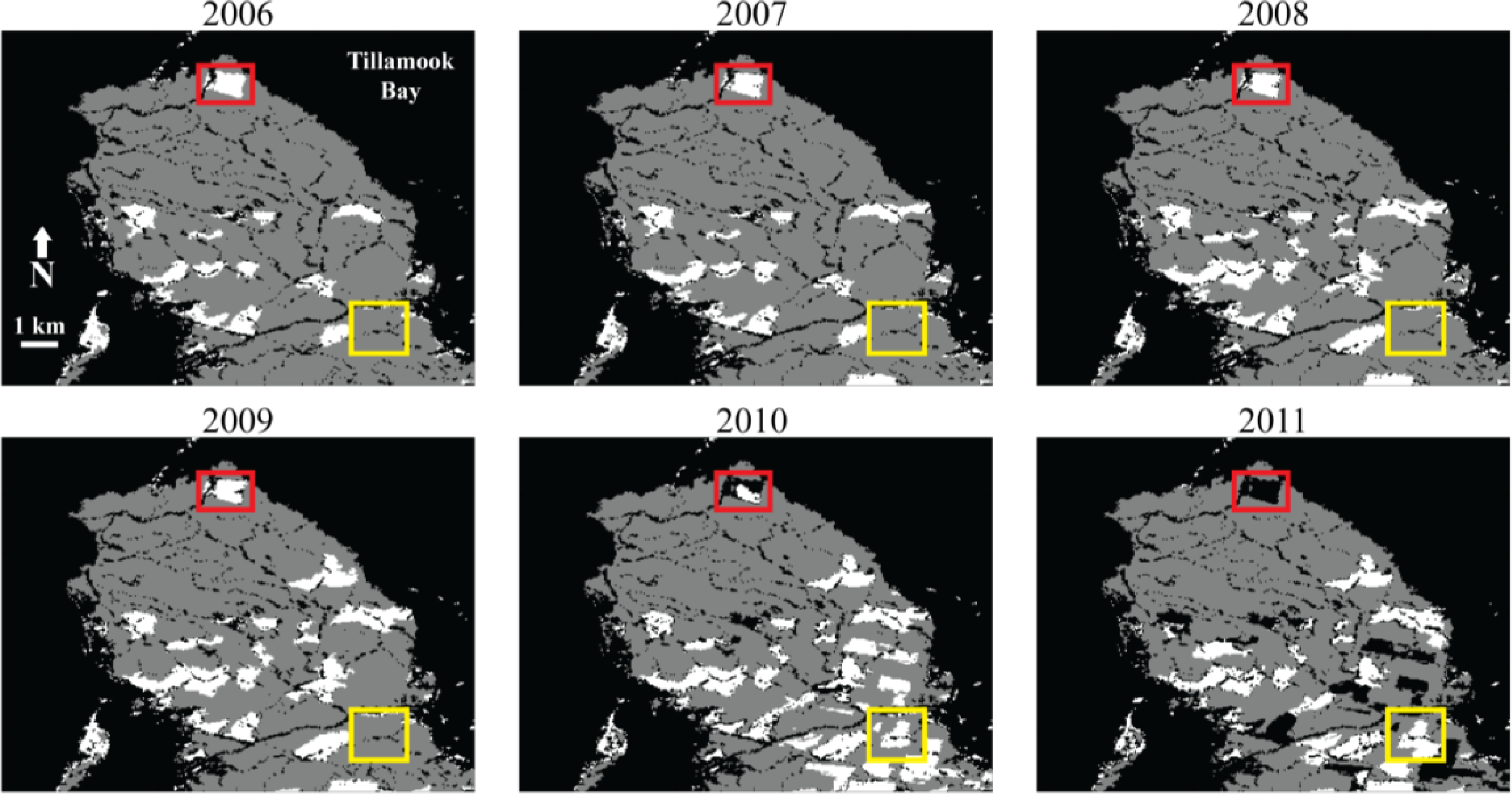
Time-varying classification of forested vs. bare (and “unclassified”) regions over the period of time covered by the SAR imagery.

(c)

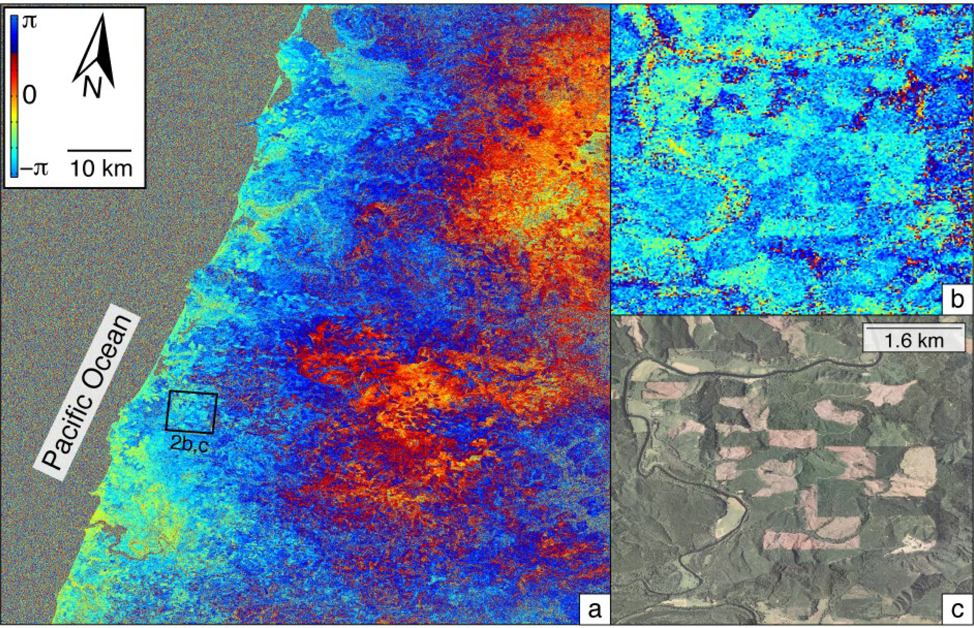
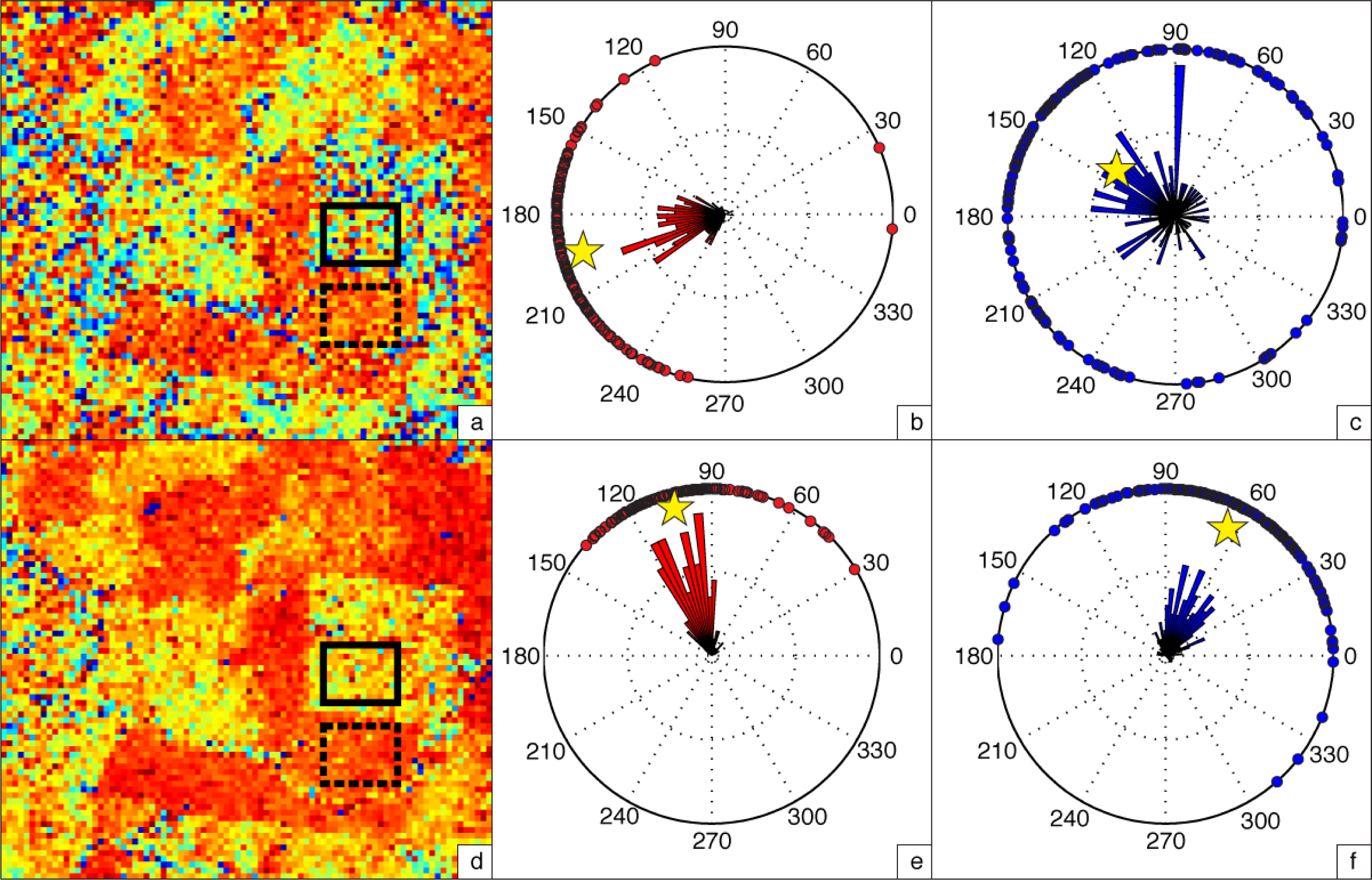
Extraction of phase information and assessment of errors on the estimated difference in interferometric phase between forested and cleared regions at individual locations within each interferogram.

(d)

Assessment of error on height estimated from full suite of interferograms at each location.

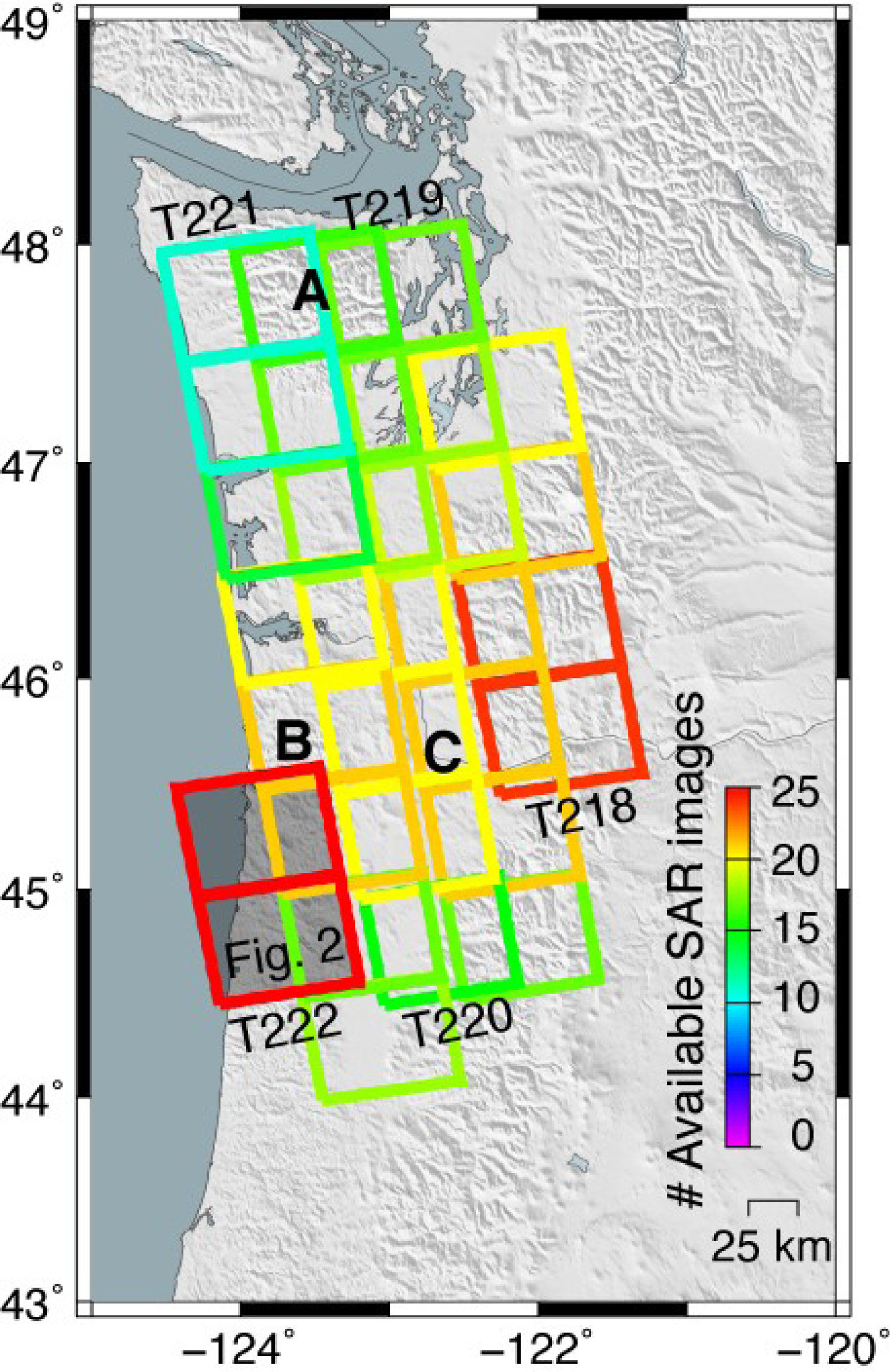
2.1. Data

We use Phased Array type L-band Synthetic Aperture Radar (PALSAR) data acquired by the ALOS satellite between January 2007 and March 2011. The number of acquisitions varies across our study area (Figure 1). We generate interferograms using the freely available Repeat Orbit Interferometry PACkage (ROI_PAC, [47]). Interferograms are downsampled (multilooked) 12 times in the azimuth direction and 4 times in the range direction. We remove topography with the 1 arc-second National Elevation Dataset (NED) product. For each frame, we generate all interferograms with B_┴ < 2500 m and temporal baselines <1 year. We rectify all interferograms to a common grid in radar range and along-track coordinates.

2.2. Automated Identification of Cleared Regions

The first critical step during our analysis is the process of determining where forests exist across the entire regions covered by our interferograms. Isolating the cleared regions used in our analysis by hand for all interferograms spanning a region as large as the Pacific Northwest would be prohibitively expensive. Instead, we use a combination of publicly available remote sensing datasets to automate classification of regions within each interferogram as “forested”, “bare” or “unclassified”. Timber harvesting occurred throughout the timespan of the available SAR data, so we include a time-variable component that ensures that we only average tree heights across time interval when no clearcutting occurred.

As part of our classification, we use the National Land Cover Database 2006 (NLCD2006) land cover product [48]. For the purposes of the canopy height estimation, we divided the NLCD2006 data into forested (classifications 41, 42 and 43) and bare (31, 52 and 71) pixels. All other classes, including water bodies (11, 12), developed regions (21, 22, 23, 24), wetlands (90, 95), and planted/cultivated regions (81, 82), are characterized as “unclassified” and are not used in our analysis.

In order to characterize the temporal variability of land cover in our study area during the 2007–2011 time frame of our study, we also use yearly Landsat 5 Thematic Mapper (LTM5) acquisitions. Cloud cover was restricted to less than 20%, and for each frame we used the least cloud- and ice-covered acquisition available for that year. We generate our augmented classification map for each year using the ratio of LTM5 band 2 (visible, 0.52–0.60 μm) and band 7 (mid-infrared, 2.08–2.35 μm). This band ratio allows identification of areas where logging occurs during the time span of our interferograms (Figure 4). However, within a few years after logging, some cleared areas regrow enough vegetation so that they are no longer flagged as “bare” by this measure. Therefore, we discard points within interferograms if they are flagged as “forested” after previously being categorized as “bare” and do not use them for the remainder of the time series analysis (black region within red box, Figure 4). Visual inspection of the data shows that this approach is very successful at identifying the state of, and changes to, the landscape, and that areas where the metric is unreliable are marked as “unclassified” (black areas, Figure 4) rather than being incorrectly flagged as forested or bare.

2.3. Estimation of Canopy Height and Associated Errors

We estimate canopy height with a running window of 40 × 40 pixels across each frame. At the resolution of the multilooked interferograms used in this study, this box corresponds to an area of approximately 1.5 km × 800 m. At each location, we extract the average phase of pixels flagged as forested or bare for each interferogram. As described above, this set of pixels is time dependent, capturing the progression of logging and regrowth at each site. Any pixels that are flagged differently for the two dates spanned by the interferogram are discarded. If the number of either forested or bare pixels for a given interferogram within the running window is below a set threshold (50 pixels), that particular interferogram will not be included in the height estimation at that location. We only generate height estimates at a given location if more than 10 interferograms meet our criteria.

Phase unwrapping—the process of converting the interferometric observations, which are “wrapped” from −π to π (Figure 5), to the total amount of range change—carries with it many potential sources of error. This is particularly true for clearcut signals, since they have a sharp boundary across which it is not clear how many cycles of phase are represented. Therefore, we estimate the average phase in the 40 × 40 window at each location within the interferograms using the full complex phase values at each pixel. We illustrate the process described below in Figure 6, but focus on the difference in phase between two small boxed regions (solid and dashed boxes in Figure 6) for clarity. The phase differences calculated using the 40 × 40 window centered on that particular set of boxes are nearly identical to those shown in Figure 6, but with smaller error bounds because of the larger number of points used.

Each pixel in an interferogram is associated with a complex phase value, φ. Because of phase wrapping, we cannot simply average the angular values of φ—a distribution that is truly centered near a value of π would result in an average value near zero, since there would be equal numbers of values near π and −π (Figure 5a,b, gray circle). However, if we treat each phase value as a complex unit vector, their average is an output vector that does capture the true mean phase of the distribution (Figure 5a,b, black circle). Conveniently, if all pixels within the averaging region have approximately the same phase value, the magnitude of φ̄ will be near unity. If the phase values are random, this magnitude will approach zero. For a wrapped Gaussian circular distribution of unit vectors, the variance of the mean, σ², is given by (e.g., [49,50]):

$${\sigma }^2=-2(\text{ln}\left|\overline{\phi }\right|)$$

(1)

At each location, we find the mean complex phase (φ̄) of all pixels within the averaging region. We estimate the mean phase for both forested (φ̄_f), and bare (φ̄_b) regions and take their difference, φ̄_d, also in the complex plane. We determine ${\sigma }_f^2$ and ${\sigma }_b^2$ for forested and bare pixel groups, respectively, with the total variance for the phase difference, φ̄_d, being the sum of the two variances. The variance of each estimate is limited by the fact that phase values are restricted to the range −π to π. Above a level of σ² ≈ 0.6 × 2π, the phase values are essentially random (Figure 5c). We use a more conservative threshold and remove all phase values for interferograms where σ² ≥ 0.45 × 2π from our analysis at each location.

The relationship between scattering phase center height and the slope, m, of the line (which goes through zero) relating phase change φ̄_d to B_┴ is related to scattering phase center height, z, as follows:

$$z=\frac{mR\text{sin}\theta \lambda }{4\pi }$$

(2)

where R is range between the satellite and ground, θ is the satellite look angle and λ is the wavelength of the sensor (e.g., [42]). Since φ̄_d is “wrapped” and can only take values between −π and π, the predicted dependence of inferred phase on baseline takes a sawtooth form. Therefore, the determination of canopy height at each location is nonlinear.

To address this nonlinearity, we perform a grid search through heights ranging from 0 to 100 m. At each height we compute the weighted root-mean-square error between the predicted and observed complex phase differences using the data variances described above, and select the height associated with lowest error at each location (Figure 7). By using the complex phase values, we avoid issues with unwrapping.

3. Results and Discussion

Our map of inferred height of the L-band phase scattering centers determined for the Pacific Northwest (Figure 7) contains several key features. The Olympic Peninsula, a region known for dense forests and tall trees, is associated with a low density of observations. This is due to forest conservation efforts over much of the Olympic Peninsula. Without cleared areas to use as a local reference for the Earth’s surface beneath the forests, height estimates cannot be made using our method. The Tillamook and Clatsop state forests in NW Oregon are similarly associated with low densities of observations. In general, our height estimates are largest within the mountain ranges, and decrease towards the eastern part of Washington and Oregon. This is not surprising, as the eastern parts of Oregon and Washington are very arid compared to the coasts. The Willamette Valley Basin, home to approximately 70% of Oregon’s population and a great deal of its agricultural production, is associated with relatively low estimated heights.

We validate our results in two ways—through comparison of adjacent satellite paths and with LiDAR data. The adjacent satellite paths used in this study overlap by ∼30 km, allowing us to assess the consistency of our results between independent sets of SAR imagery (Figure 8). The 1σ error bounds for nearby height estimates from different tracks overlap in most instances. In Figure 8, we illustrate the errors on height for both a pixel where the estimates from overlapping tracks agree well (point B) and where they differ by a significant amount (point C). Examination of the error bounds show that the discrepancy at point C results from a larger uncertainty on the heights at that location. This could be due to several factors—the two tracks will likely contain a different number of interferograms that sample different dates, and one set may have experienced more decorrelation or changes in land use than the other.

The L-band (λ = 23.6 cm) radar data provided by ALOS does not interact with the very top of the canopy, so we expect the apparent heights to be lower than those obtained in the field, from LiDAR data, or by using C- or X-band SAR sensors [28]. The scattering phase center for a given sensor and location will vary depending on factors such as forest density, canopy morphology, wavelength, and incident angle of the sensor (e.g., [51–53]). We find that our inferred canopy heights are consistently ∼50% smaller than LiDAR-based height estimates using data obtained by the Oregon Department of Geology and Mineral Industries (DOGAMI), available online through the NSF OpenTopography Facility (Figure 9), a result that is consistent with the expected depth of interaction for L-band SAR [28]. Application of our approach to global climate studies would require further calibration of the relationship between estimates of the L-band based phase scattering height and stored biomass, as is necessary for most metrics.

While our approach compares pixels using a binary “cleared” or “forested” approach, many regions in the Pacific Northwest have been harvested sequentially at different times in the past decades. Adjacent plots of land often contain trees with substantially different heights (Figure 9), resulting in sharp phase boundaries between regions that are all treated as “forested” by our algorithm. Currently, our method extracts an average height for these regions of multi-stage regrowth. As data quality improves and the number of available SAR acquisitions in the archive increases, it may be possible to assess these effects by examining the confidence intervals on our height estimates. Given a sufficiently long time span of SAR acquisitions, determination of changing canopy height as trees regrow after clearcutting should be possible.

4. Conclusions

Monitoring of forest stock globally and at frequent time intervals is critical to efforts to study and mitigate anthropogenic effects on climate change. We have presented a method for determining regional the height of the L-band phase scattering center using phase differences between adjacent cleared and forested regions observed in L-band interferograms. Our method is restricted to regions that have undergone clearing within the past few years, providing no canopy height estimates in other regions of importance, such as protected forests. We combine the available SAR imagery with time-variable maps of landcover, allowing us to automatically extract differences in phase over large areas without the time-consuming process of hand-picking targets. As described above, in cases where we benchmark the automated approach against hand-chosen forested and cleared regions, the results are indistinguishable.

Our approach also uses the full complex interferometric phase values (instead of unwrapped values) to estimate the error on the average phase estimates in each region. This avoids phase-unwrapping errors that would occur frequently due to the high phase gradient that occurs between forested and clearcut areas. The errors on our height estimates depend on the data coverage at each location, but are typically around 5 m. We compare our results between overlapping InSAR tracks with completely independent sets of SAR imagery and demonstrate that the inferred heights are consistent within our stated errors. Comparisons with LiDAR-based tree heights (difference between first and ground returns) suggest that the L-band height is ∼50% of the total height, a result that is consistent with previous work. Further calibration work would be needed before this method could be used to estimate characteristics of carbon stocks, including examination of the effects of tree spacing, species, and identification of any seasonal variation. The existing data catalog is not optimized for this sort of work—unfortunately, areas dominated by different tree species, such as the eastern United States, were only observed by the ALOS satellite around 5 times. We anticipate that the upcoming ALOS-2 mission, set to launch in early 2014, will extend this catalog. A strength of this approach is that it can be applied at any time of day or under any cloud cover conditions, and in regions with high biomass or steep slopes, where application of other approaches that rely on remote sensing can be challenging.

The steadily growing catalog of publicly available SAR imagery will allow further improvement to this and other SAR-based approaches. The assimilation of C- or X-band data would allow better constraints on canopy height than would be possible using L-band-based proxies alone. Shorter repeat intervals such as those proposed for satellites set to launch in upcoming years will result in improved coherence and time series that can better identify changes in forest coverage and heights.

References

1. Dixon, R.K.; Solomon, A.M.; Brown, S.; Houghton, R.A.; Trexier, M.C.; Wisniewski, J. Carbon pools and flux of global forest ecosystems. Science 1994, 263, 185–190. [Google Scholar]
2. Denman, K.L.; Brasseur, G.; Chidthaisong, A.; Ciais, P.; Cox, P.; Dickinson, R.E.; Haugustaine, D.; Heinze, C.; Holland, E.; Jacob, D.; et al. Couplings between Changes in the Climate System and Biogeochemistry. In Climate Change 2007: The Physical Science Basis. Contribution of Working Group I to the Fourth Assessment Report of the Intergovernmental Panel on Climate Change; Solomon, S., Qin, D., Manning, M., Chen, Z., Marquis, M., Averyt, K.B., TIgnor, M., Miller, H.L., Eds.; Cambridge University Press: Cambridge, UK; New York, NY, USA, 2007; pp. 499–587. [Google Scholar]
3. Gullison, R.E.; Frumhoff, P.C.; Canadell, J.G.; Field, C.B.; Nepstad, D.C.; Hayhoe, K.; Avissar, R.; Curran, L.M.; Friedlingstein, P.; Jones, C.D.; et al. Tropical forests and climate policy. Science 2007, 316, 985–986. [Google Scholar]
4. Lindquist, E.J.; D’Annunzio, R.; Gerrand, A.; MacDicken, K.; Achard, F.; Beuchle, R.; Brink, A.; Eva, H.D.; Mayaux, P.; San-Miguel-Ayanz, J. Global Forest Land-Use Change 1990–2005; FAO Forestry Paper; Food and Agriculture Organization of the United Nations and European Commission Joint Research Centre: Rome, Italy, 2012. [Google Scholar]
5. Van der Werf, G.R.; Morton, D.C.; DeFries, R.S.; Olivier, J.G.J.; Kasibhatla, P.S.; Jackson, R.B.; Collatz, G.J.; Randerson, J.T. CO2 emissions from forest loss. Nat. Geosci 2009, 2, 737–738. [Google Scholar]
6. Goetz, S.J.; Baccini, A.; Laporte, N.T.; Johns, T.; Walker, W.; Kellndorfer, J.; Houghton, R.A.; Sun, M. Mapping and monitoring carbon stocks with satellite observations: A comparison of methods. Carbon Balanc. Manag 2009, 4. [Google Scholar] [CrossRef]
7. Solberg, S.; Astrup, R.; Gobakken, T.; Næsset, E.; Weydahl, D.J. Estimating spruce and pine biomass with interferometric X-band SAR. Remote Sens. Environ 2010, 114, 2353–2360. [Google Scholar]
8. Sandberg, G.; Ulander, L.M.H.; Fransson, J.E.S.; Holmgren, J.; le Toan, T. L- and P-band backscatter intensity for biomass retrieval in hemiboreal forest. Remote Sens. Environ 2011, 115, 2874–2886. [Google Scholar]
9. Lynch, J.; Maslin, M.; Balzter, H.; Sweeting, M. Sustainability: Choose satellites to monitor deforestation. Nature 2013, 496, 293–294. [Google Scholar]
10. Dubayah, R.O.; Drake, J.B. Lidar remote sensing for forestry. J. For 2000, 98, 44–46. [Google Scholar]
11. Andersen, H.E.; McGaughey, R.J.; Carson, W.W.; Reutebuch, S.E.; Mercer, B.; Allan, J. A comparison of forest canopy models derived from LIDAR and INSAR data in a Pacific Northwest conifer forest. Int. Arch. Photogramm. Remote Sens 2003, 34, 211–217. [Google Scholar]
12. Kellndorfer, J.; Walker, W.; Pierce, L.; Dobson, C.; Fites, J.A.; Hunsaker, C.; Vona, J.; Clutter, M. Vegetation height estimation from Shuttle Radar Topography Mission and National Elevation Datasets. Remote Sens. Environ 2004, 93, 339–358. [Google Scholar]
13. Sun, G.; Ranson, K.J.; Kimes, D.S.; Blair, J.B.; Kovacs, K. Forest vertical structure from GLAS: An evaluation using LVIS and SRTM data. Remote Sens. Environ 2008, 112, 107–117. [Google Scholar]
14. Gatziolis, D.; Fried, J.S.; Monleon, V.S. Challenges to estimating tree height via LiDAR in closed-canopy forest: A parable from western Oregon. For. Sci 2010, 56, 139–155. [Google Scholar]
15. Kellndorfer, J.M.; Walker, W.S.; LaPoint, E.; Kirsch, K.; Bishop, J.; Fiske, G. Statistical fusion of lidar, InSAR, and optical remote sensing data for forest stand height characterization: A regional-scale method based on LVIS, SRTM, Landsat ETM+, and ancillary data sets. J. Geophys. Res 2010, 115. [Google Scholar] [CrossRef]
16. Lefsky, M.A. A global forest canopy height map from the Moderate Resolution Imaging Spectroradiometer and the Geoscience Laser Altimeter System. Geophys. Res. Lett 2010, 37. [Google Scholar] [CrossRef]
17. Saatchi, S.S.; Harris, N.L.; Brown, S.; Lefsky, M.; Mitchard, E.T.A.; Salas, W.; Zutta, B.R.; Buermann, W.; Lewis, S.L.; Hagen, S.; et al. Benchmark map of forest carbon stocks in tropical regions across three continents. Proc. Natl. Acad. Sci. USA 2011, 108, 9899–9904. [Google Scholar]
18. Simard, M.; Pinto, N.; Fisher, J.B.; Baccini, A. Mapping forest canopy height globally with spaceborne lidar. J. Geophys. Res 2011, 116. [Google Scholar] [CrossRef]
19. Mitchard, E.T.A.; Saatchi, S.S.; White, L.J.T.; Abernethy, K.A.; Jeffery, K.J.; Lewis, S.L.; Collins, M.; Lefsky, M.A.; Leal, M.E.; Woodhouse, I.H.; et al. Mapping tropical forest biomass with radar and spaceborne LiDAR in Lope National Park, Gabon: Overcoming problems of high biomass and persistent cloud. Biogeosciences 2012, 9, 179–191. [Google Scholar]
20. Dobson, M.C.; Ulaby, F.; LeToan, T.; Beaudoin, A.; Kasischke, E.S.; Christensen, N. Dependence of radar backscatter on coniferous forest biomass. IEEE Trans. Geosci. Remote Sens 1992, 30, 412–415. [Google Scholar]
21. Dobson, M.C.; Ulaby, F.; Pierce, L.; Bergen, K.; Kellndorfer, J.; Kendra, J.; Li, E.; Lin, Y.; Nashasihibi, A.; Sarabandi, K.; et al. Estimation of forest biophysical characteristics in Northern Micigan with SIR-C/X-SAR. IEEE Trans. Geosci. Remote Sens 1995, 33, 877–895. [Google Scholar]
22. Cloude, S.R.; Papathanassiou, K.P. Polarimetric SAR interferometry. IEEE Trans. Geosci. Remote Sens 1998, 36, 1551–1565. [Google Scholar]
23. Treuhaft, R.N.; Law, B.E.; Asner, G.P. Forest attributes from radar interferometric structure and its fusion with optical remote sensing. BioScience 2004, 54, 561–571. [Google Scholar]
24. Thiel, C.J.; Thiel, C.; Schmullius, C.C. Operational large-area forest monitoring in Siberia using ALOS PALSAR summer intensities and winter coherence. IEEE Trans. Geosci. Remote Sens 2009, 47, 3993–4000. [Google Scholar]
25. Asner, G.P.; Powell, G.V.N.; Mascaro, J.; Knapp, D.E.; Clark, J.K.; Jacobson, J.; Kennedy-Bowdoin, T.; Balaji, A.; Paez-Acosta, G.; Victoria, E.; et al. High-resolution forest carbon stocks and emissions in the Amazon. Proc. Natl. Acad. Sci. USA 2010, 107, 16738–16742. [Google Scholar]
26. Kovats, M. A large-scale aerial photographic technique for measuring tree heights on long-term forest installations. Photogramm. Eng. Remote Sens 1997, 63, 741–747. [Google Scholar]
27. Balzter, H.; Luckman, A.; Skinner, L.; Rowland, C.; Dawson, T. Observations of forest stand top height and mean height from interferometric SAR and LiDAR over a conifer plantation at Thetford Forest, UK. Int. J. Remote Sens 2007, 28, 1173–1197. [Google Scholar]
28. Sexton, J.O.; Bax, T.; Siqueira, P.; Swenson, J.J.; Hensley, S. A comparison of lidar, radar, and field measurements of canopy height in pine and hardwood forests of southeastern North America. For. Ecol. Manag 2009, 257, 1136–1147. [Google Scholar]
29. Wulder, M.A.; White, J.C.; Nelson, R.F.; Næsset, E.; Ørka, H.O.; Coops, N.C.; Hilker, T.; Bater, C.W.; Gobakken, T. Lidar sampling for large-area forest characterization: A review. Remote Sens. Environ 2012, 121, 196–209. [Google Scholar]
30. Baltsavias, E.P. Airborne laser scanning: Basic relations and formulas. ISPRS J. Photogramm. Remote Sens 1999, 54, 199–214. [Google Scholar]
31. Asner, G.P.; Knapp, D.E.; Broadbent, E.N.; Oliveira, P.J.C.; Keller, M.; Silva, J.N. Selective logging in the Brazilian Amazon. Science 2005, 310, 480–482. [Google Scholar]
32. Breidenbach, J.; Koch, B.; Kandler, G.; Kleusberg, A. Quantifying the influence of slope, aspect, crown shape and stem density on the estimation of tree height at plot level using lidar and InSAR data. Int. J. Remote Sens 2008, 29, 1511–1536. [Google Scholar]
33. Burgmann, R.; Rosen, P.A.; Fielding, E.J. Synthetic aperture radar interferometry to measure Earth’s surface topography and its deformation. Annu. Rev. Earth Planet. Sci 2000, 28, 169–209. [Google Scholar]
34. Igarashi, T. Alos mission requirement and sensor specifications. Adv. Space Res 2001, 28, 127–131. [Google Scholar]
35. Hagberg, J.O.; Ulander, L.M.H.; Askne, J. Repeat-pass SAR interferometry over forested terrain. IEEE Trans. Geosci. Remote Sens 1995, 33, 331–340. [Google Scholar]
36. Treuhaft, R.N.; Madsen, S.N.; Moghaddam, M.; van Zyl, J.J. Vegetation characteristics and underlying topography from interferometric radar. Radio Sci 1996, 31, 1449–1485. [Google Scholar]
37. Askne, J.I.H.; Dammert, P.B.G.; Ulander, L.M.H.; Smith, G. C-band repeat-pass interferometric SAR observations of the forest. IEEE Trans. Geosci. Remote Sens 1997, 35, 25–35. [Google Scholar]
38. Wegmuller, U.; Werner, C. Retrieval of vegetation parameters with SAR interferometry. IEEE Trans. Geosci. Remote Sens 1997, 35. [Google Scholar] [CrossRef]
39. Walker, W.; Kellndorfer, J.; Pierce, L. Quality assessment of SRTM C- and X-band interferometric data: Implications for the retrieval of vegetation canopy height. Remote Sens. Environ 2007, 106, 428–448. [Google Scholar]
40. Zebker, H.A.; Villasenor, J. Decorrelation in interferometric radar echoes. IEEE Trans. Geosci. Remote Sens 1992, 30, 950–959. [Google Scholar]
41. Zebker, H.A.; Rosen, P.A.; Hensley, S. Atmospheric effects in interferometric synthetic aperture radar surface deformation and topographic maps. J. Geophys. Res 1997, 102, 7547–7563. [Google Scholar]
42. Hanssen, R.F. Radar Interferometry: Data Interpretation and Error Analysis; Springer: Dordrecht, The Netherlands, 2001. [Google Scholar]
43. Emardson, T.R.; Simons, M.; Webb, F.H. Neutral atmospheric delay in interferometric synthetic aperture radar applications: Statistical description and mitigation. J. Geophys. Res 2003, 108. [Google Scholar] [CrossRef]
44. Lohman, R.B.; Simons, M. Some thoughts on the use of InSAR data to constrain models of surface deformation: Noise structure and data downsampling. Geochem. Geophys. Geosyst 2005, 6. [Google Scholar] [CrossRef]
45. Zebker, H.A.; Goldstein, R.M. Topographic mapping from interferometric synthetic aperture radar observations. J. Geophys. Res 1986, 91, 4993–4999. [Google Scholar]
46. Rodriguez, E.; Martin, J.M. Theory and design of interferometric synthetic aperture radars. IEEE Proc. Radar Signal Process 1992, 139, 147–159. [Google Scholar]
47. Rosen, P.A.; Hensley, S.; Peltzer, G.; Simons, M. Updated repeat orbit interferometry package released. EOS 2004, 85. [Google Scholar] [CrossRef]
48. Fry, J.A.; Dewitz, J.; Homer, C.J.; Xian, G.; Jin, S.; Yang, L.; Barnes, C.A.; Herold, N.D.; Wickham, J.D. Completion of the 2006 national land cover database for the conterminous united states. Photogramm. Eng. Remote Sens 2011, 77, 858–864. [Google Scholar]
49. Fisher, N.I. Statistical Analysis of Circular Data; Cambridge University Press: Cambridge, UK, 1995. [Google Scholar]
50. Mardia, K.V.; Jupp, P.E. Directional Statistics, 1st ed; Wiley: Hoboken, NJ, USA, 1999. [Google Scholar]
51. Sarabandi, K.; Lin, Y.-C. Simulation of interferometric SAR response for characterizing the scattering phase center statistics of forest canopies. IEEE Trans. Geosci. Remote Sens 2000, 38, 115–125. [Google Scholar]
52. Izzawati; Wallington, E.D.; Woodhouse, I.H. Forest height retrieval from commercial X-band SAR products. IEEE Trans. Geosci. Remote Sens 2006, 44, 863–870. [Google Scholar]
53. Andersen, H.-E.; McGaughey, R.; Reutebuch, S. Assessing the influence of flight parameters, interferometric processing, slope and canopy density on the accuracy of X-band IFSAR-derived forest canopy height models. Int. J. Remote Sens 2008, 29, 1495–1510. [Google Scholar]
Figure 1. Study region and data coverage. Colored boxes indicate the extent of coverage and data density of the five tracks of L-band synthetic aperture radar (SAR) data used in this study. A: Olympic Peninsula; B: Tillamook and Clatsop State Forests; C: Willamette Valley Basin. Area shown in Figure 2 is shaded gray.
Remotesensing 06 03210f1
Figure 2. Example wrapped interferogram (a) from our study region (track 222, frame 890), spanning 18 July—2 September 2009 with perpendicular baseline, B = 470 m, displayed in radar coordinates (Location in Figure 1, distance scale approximate). Phase values over water (Pacific Ocean) are decorrelated/random. Box indicates location of comparison between phase (b) and optical imagery (c).
Remotesensing 06 03210f2
Figure 3. Two cleared regions (top and bottom rows, respectively) observed in three interferograms. Dates and B for each: (a,e) 14 April—30 May 2008; −139 m (b,f) 28 November 2007–13 January 2008; 517 m (c,g) 30 November 2008–15 January 2009; 566 m. Each panel is 3 km × 3 km; (d,h) Phase difference between hand-picked bare (dashed box) and forested (solid box) regions for all interferograms (black dots) vs. B, with the three interferograms shown here highlighted in yellow. Red and blue bars indicate the 1σ values of phase for bare and forested pixels, respectively. Note larger errors on forested pixels, due to volumetric decorrelation. Solid and dashed lines indicate best-fit height and 1σ error bounds, respectively.
Remotesensing 06 03210f3
Figure 4. Example of temporal variability of Landsat-based classification as bare (white), forested (gray) and unclassified (black). Red box indicates region marked as “bare” at the beginning of the time series, but that had grown enough vegetation by the end to be classified as “forested”. We remove pixels that change from “bare” to “forested” during the time series. Yellow box indicates a region that was harvested between 2009 and 2010.
Remotesensing 06 03210f4
Figure 5. (a) Simulated histogram of wrapped phase values in radians, with σ = 0.3π (heavy black line). Average value estimated from real-valued phase (gray circle) is offset from the true value (black circle); (b) Data from (a) shown on complex plane (rose diagram, scaled to max = 1). Amplitude of complex-averaged value (black circle) increases as σ approaches 0. Gray circle as in (b); (c) Inferred σ (Equation (1)) using simulated noise with a range of input σ, wrapped at −π to π. Inferred σ saturates above a threshold of ∼0.6 × 2π. Black dotted line indicates 1:1 relationship and horizontal gray dashed line indicates the cutoff we use in our analysis.
Remotesensing 06 03210f5
Figure 6. Comparison of variance in phase (a,d) between interferograms of varying quality (top row, 18 October 2009–18 January 2010, B = 603, bottom row, 30 November 2008–15 January 2009, B = 566) for the same 2.5 km × 2.5 km region. Note that they have similar baselines, so we expect the phase difference between hand-picked bare (dashed line) and forested (solid line) regions to be similar. Phase values for all pixels within the cleared (b,e) and forested (c,f) regions (dots, rose diagram) on the complex plane show different amounts of spread, with cleared regions having less noise on average. Yellow stars in each plot indicate the average complex phase, (φ̄), which will have a smaller magnitude (closer to origin) if there is a large spread in phase values.
Remotesensing 06 03210f6
Figure 7. Study region and inferred phase center heights. Black boxes indicate the five tracks of L-band SAR data used in this study. A: Olympic Peninsula; B: Tillamook and Clatsop State Forests; C: Willamette Valley Basin. Colored dots indicate the inferred height of the L-band phase scattering center at each location.
Remotesensing 06 03210f7
Figure 8. Comparison of inferred phase scattering center height (a) between two overlapping tracks, T221 (circles) and T222 (stars), overlain on digital orthophoto quad (grayscale). Color indicates height in meters; The error bounds (shaded) on heights (solid red, black lines) for two points where nearby estimates are similar (b) and dissimilar (c) overlap at the 1σ level.
Remotesensing 06 03210f8
Figure 9. Comparison of InSAR- and LiDAR-based results. (a,b) LiDAR-based canopy height map (difference between first and ground return) covering two different areas (color) and location of profiles X-X’ (white dashed lines, box shows total area sampled) used in (c,d). Profiles show elevation of ground return (red), individual first returns (trees, green dots) from the LiDAR data. Blue curve indicates the InSAR-based height, offset from the LiDAR-based ground surface. Note that the InSAR height is an average estimated over the entire area shown in panels (a,b).
Remotesensing 06 03210f9