Object-Based Greenhouse Classification from GeoEye-1 and WorldView-2 Stereo Imagery

Abstract

Remote sensing technologies have been commonly used to perform greenhouse detection and mapping. In this research, stereo pairs acquired by very high-resolution optical satellites GeoEye-1 (GE1) and WorldView-2 (WV2) have been utilized to carry out the land cover classification of an agricultural area through an object-based image analysis approach, paying special attention to greenhouses extraction. The main novelty of this work lies in the joint use of single-source stereo-photogrammetrically derived heights and multispectral information from both panchromatic and pan-sharpened orthoimages. The main features tested in this research can be grouped into different categories, such as basic spectral information, elevation data (normalized digital surface model; nDSM), band indexes and ratios, texture and shape geometry. Furthermore, spectral information was based on both single orthoimages and multiangle orthoimages. The overall accuracy attained by applying nearest neighbor and support vector machine classifiers to the four multispectral bands of GE1 were very similar to those computed from WV2, for either four or eight multispectral bands. Height data, in the form of nDSM, were the most important feature for greenhouse classification. The best overall accuracy values were close to 90%, and they were not improved by using multiangle orthoimages.

1. Introduction

Since the first plastic-covered greenhouses were built in agriculture on a significant scale by the early 1950s, the area covered by them has been increasing at a fast rate [1]. North Africa, the Middle East and China are growing at 15%–30% annually, while Europe (mainly Spain, Italy and France) presents a much lower increase. Currently, there are about 1,600,000 ha of greenhouses and walk-in tunnels scattered all over the world [1].

The practice of plastic-covered agriculture, also known as plasticulture, is part of the transformation of conventional farming into a more industrial and high-tech precision agriculture [2]. It is widely recognized that this type of cultivation is linked to a very important anthropic impact [3]. In fact, the construction of greenhouses, together with the necessary infrastructure for their commercial exploitation (e.g., road networks, rural buildings, reservoirs and irrigation ponds), contribute to affecting the environment [4]. Therefore, a careful spatial development planning is required in these agricultural areas to minimize their environmental impact [4–6].

Automatic mapping of greenhouses from remote sensing methods presents a special challenge, due to their unique characteristics [2,5,7–9]. In fact, the spectral signature of plastic changes drastically depending on: (i) the plastic material (i.e., thickness, density, transparency, light dispersal, ultraviolet and infrared properties, anti-fog additives and color); (ii) seasonal use of greenhouses (e.g., during summer, polyethylene sheets may be painted white to protect plants against excessive radiation and to lower the temperature inside the greenhouse); (iii) changing the reflectance of the vegetation underneath, which contributes to the overall reflectance of the greenhouse; and (iv) the angle of vision (i.e., the relationship between the light incidence angle and the remote sensor point of view). All these factors may result in different spectral signatures for the same type of land use, which entails a serious risk of confusion with other non-greenhouse classes.

The first works focused on greenhouses detection from satellite data were supported by Landsat Thematic Mapper images. Some of them were carried out in the Netherlands [10,11], in a coastal province of eastern China, named Shandong [12], in southeastern Spain [13] and in Southern Italy [6]. However, the main problem of using Landsat images is related to their large pixel size or ground sample distance (GSD). With the advent of the first very high-resolution (VHR) commercial satellites, such as IKONOS and QuickBird, in 1999 and 2001, respectively, the aforementioned problem was solved. In fact, these VHR satellites are capable of capturing panchromatic (PAN) imagery of the land surface with GSD even lower than 1 m. To date, only a few works based on the detection of plastic greenhouses from IKONOS or QuickBird images have been performed [5,7,14–17] by using different pixel-based approaches.

More recently, a new breed of VHR satellites with improved geometric and radiometric characteristics has been successfully launched. Among them, GeoEye-1 (GE1) and WorldView-2 (WV2) are the most innovative. Although this couple of sensors has been already tested for automatic classification of urban environments and building extraction [18–21], their application to greenhouse detection is limited. In fact, only a recent work by Koc-San [22] uses WV2 satellite imagery for the pixel-based classification of glass and plastic greenhouses in Antalya (Turkey).

Regarding VHR satellite imagery, it is worth noting that the higher geometric detail of the PAN image and the useful color information provided by the lower resolution multispectral (MS) image can be fused to produce a final pan-sharpened MS image with the geometric resolution of the PAN band [23]. With the availability of pan-sharpened VHR satellite imagery, the classification of small-scale man-made structures has become of great interest. In this way, object-based image analysis (OBIA) has recently proved to be an effective approach to deal with classification tasks, especially in urban environments [24–27]. OBIA does not use individual pixels, but pixel groups representing meaningful segments (or objects), which have been segmented according to different criteria before carrying out the classification stage. Furthermore, unlike traditional pixel-based methods that only use spectral information, object-based approaches benefit from different features, such as shape, texture and context information associated with the objects [24]. At this point, and regarding remote sensing image analysis, it should be clearly stated that much of the work referred to as OBIA has been originated around the software known as eCognition (Trimble, Sunnyvale, California, United States). Indeed, about half of the papers related to OBIA are based on this package [24]. To the authors’ knowledge, OBIA has been only used for greenhouse detection by Arcidiacono and Porto [28] and Tarantino and Figorito [9]. Both works applied OBIA techniques to detect plastic greenhouses from digital true color (RGB) aerial data in different study areas of Italy (Ragusa, Scicli and Apulia Region). In these last two works, a very good review about plasticulture extraction from remote sensing imagery was carried out.

Several works have combined MS imagery and height information, often derived from LiDAR data, to improve building automatic detection [29–31]. In fact, the inclusion of elevation data increases the ability to differentiate objects with significant height, as compared with other spectrally similar classes [19]. However, LiDAR data are often expensive, and they are not always available, especially in developing countries. Nowadays, the adaptable stereo imaging capability of the newest civilian VHR satellites and their improved geometric resolution allow the generation of very accurate digital surface models (DSM) by means of standard photogrammetric procedures. In the cases of GE1 and WV2, a vertical accuracy ranging from 0.4 m to 1.2 m has been reported in the literature [32–34]. In this way, some authors have recently used single-source height and MS or pan-sharpened information from satellite platforms headed up to detailed urban classification or change detection studies [19,21,35,36].

In the case of greenhouse detection, 2D information delivered by satellite images is often not sufficient. For example, it is sometimes difficult to distinguish white plastic greenhouses from white buildings, due to their similar spectral characteristics [10]. Likewise, greenhouses only covered by a shadow net film can also be confused with bare soil [13]. In order to address this problem, and bearing in mind the aforementioned capabilities of satellite stereo imagery to provide height data, the joint use of 2D and 3D information from VHR stereo pairs seems to be a promising approach.

Moreover, the use of multiangle images has significantly improved the classification over the base case of a single nadir multispectral image [19,37]. These improvements could be due to the marked angular and directional variation of the reflectance for certain surfaces. In fact, a multiangle data set from MS WV2 images allowed the differentiation of classes not typically well identified from a single image, such as skyscrapers, bridges and flat and pitched roofs [19]. Duca and Del Frate [37] also reported significant improvements in the accuracy of asphalt, buildings and bare soil class detection from using the multiangle CHRIS-PROBA images (18 m GSD) with respect to the nadir acquisition.

Therefore, the goal of this article is strictly focused on comparing, in almost the same conditions, land cover classification accuracy with emphasis on greenhouses between VHR satellite stereo pairs from GE1 and WV2 by using the most complete data sets that can be retrieved from them (i.e., evaluating the implications of adding height and multiangle data to the information contained in a single and near-nadir image). The main novelty of this work lies in the joint use of spectral information from both PAN and pan-sharpened multiangle orthoimages and height data extracted by stereo matching from satellite stereo pairs to greenhouse classification through an OBIA approach. The spectral information includes features grouped into different categories, such as basic spectral information, band indexes and ratios, texture and the shape geometry of objects.

2. Study Area and Data Sets

2.1. Study Site

The study area is located in the municipality of Cuevas del Almanzora, province of Almería, southern Spain (Figure 1). It comprises a rectangular area of about 680 ha around the village of Palomares and is centered on the WGS84 geographic coordinates of 37.2465°N and 1.7912°W.

The land use between the urban area of Palomares and the Almanzora River is predominantly agricultural. In August 2011, the study area housed 124 greenhouses, which showed great heterogeneity. Thirty-three of them were covered by plastic material and the rest with different types of mesh or shadow net film. While some of them were being prepared for setting a new crop (i.e., they remained uncropped at the time when the satellite image was taken), others were dedicated to nurseries, and the rest housed different crops underneath (e.g., watermelon, melon, tomato, pepper and cut flowers).

2.2. Data Sets

The experimental data sets consist of two stereo pairs from GE1 and WV2 captured over the same study area and very close dates. From these stereo pairs, both orthoimages (2D information) and DSMs (3D information) were generated.

Currently, GE1 is the commercial satellite with the highest geometric resolution, presenting 0.41 m GSD at nadir in PAN mode and 1.65 m GSD at nadir in multispectral (MS) imagery. It includes the four classic bands: blue (B, 450–510 nm), green (G, 510–580 nm), red (R, 655–690 nm) and near-infrared (NIR, 780–920 nm). On the other hand, WV2 (0.46 m and 1.84 m GSD in PAN and MS modes, respectively) is the first commercial VHR satellite providing 8 bands in MS mode. In this sense, it is able to capture the four classical bands already contained in the MS image of its predecessors, i.e., B (450–510 nm), G (510–580 nm), R (630–690 nm) and near-infrared-1 or NIR1 (760–895 nm), and four additional bands, such as coastal (C, 400–450 nm), yellow (Y, 585–625 nm), red edge (RE, 705–745 nm) and near-infrared-2 (NIR2, 860–1,040 nm). Images from either GE1 or WV2 have to be down-sampled to 0.5 m and 2 m, in PAN and MS modes, respectively, for commercial sales, as required by the US Government.

The first stereo pair from WV2 was acquired on 18 August 2011 (

Table 1. Characteristics of WV2 and GE1 stereo pairs acquired over the study site. ORS2A, Ortho Ready Standard Level-2A. PAN, panchromatic; MS, multispectral.

Product	WV2 ORS2A		GE1 GeoStereo
Image ID	WV22	WV10	GE9	GE23
Acquisition Date	8/18/2011	8/18/2011	8/27/2011	8/27/2011
Acquisition Time (GTM)	11:22	11:23	10:55	10:56
Cloud Cover	0%	0%	0%	0%
Scan Direction	Forward	Reverse	Reverse	Reverse
Sun Azimuth	152.3°	152.8°	144.1°	144.4°
Sun Elevation	63.7°	63.8°	58.3°	58.4°
Collection Azimuth	4.7°	216.1°	40.4 °	183.6°
Collection Elevation	67.6°	80.0°	81.5 °	66.9°
Off-nadir	22.4°	10.0°	8.5 °	23.1°
Product Pixel Size (PAN)	0.5 m	0.5 m	0.5 m	0.5 m
Product Pixel Size (MS)	2 m	2 m	2 m	2 m

), presenting a convergence angle of 31.35°. It was collected in Ortho Ready Standard Level-2A (ORS2A) format, containing both PAN and MS imagery. WV2 ORS2A images present both radiometric and geometric corrections. They are georeferenced to a cartographic projection using a surface with constant height and include the corresponding RPC sensor camera model and metadata file. The delivered products were ordered with a dynamic range of 11 bits and without the application of the dynamic range adjustment (DRA) preprocessing (i.e., maintaining absolute radiometric accuracy and the full dynamic range for scientific applications).

The second stereo pair was collected on 27 August 2011 (Table 1). It was a bundle (PAN + MS) GeoStereo product from GE1 presenting a convergence angle of 30.39°. GE1 GeoStereo images present both radiometric and geometric corrections similar to those applied to WV2 ORS2A imagery. The delivered products had a dynamic range of 11 bits and without DRA preprocessing. The Sun position, the satellite track (north-south) and the stereo geometry of this GeoStereo product were similar to those configuring the aforementioned WV2 stereo pair. However, the first image in the case of the GE1 stereo pair had an off-nadir of 8.5° (the most single nadir image) and the second 23.1°, while in the WV2 case, the second image was the most vertical or near-nadir.

Besides the two described stereo pairs, a medium resolution 10-m grid spacing digital elevation model (DEM) was used. It was compiled from a B&W photogrammetric flight at an approximate scale of 1:20,000 and undertaken by the Andalusia Government. This DEM presented an estimated vertical accuracy of 1.34 m measured as root mean square error (RMSE). Finally, publicly available information, 0.5 m GSD aerial orthophotographs (true color RGB) were also used in this work. They were taken and made in 2010 as part of the Spanish Programme of Aerial Orthophotography (PNOA).

3. Methodology

3.1. Pre-Processing of Data Sets

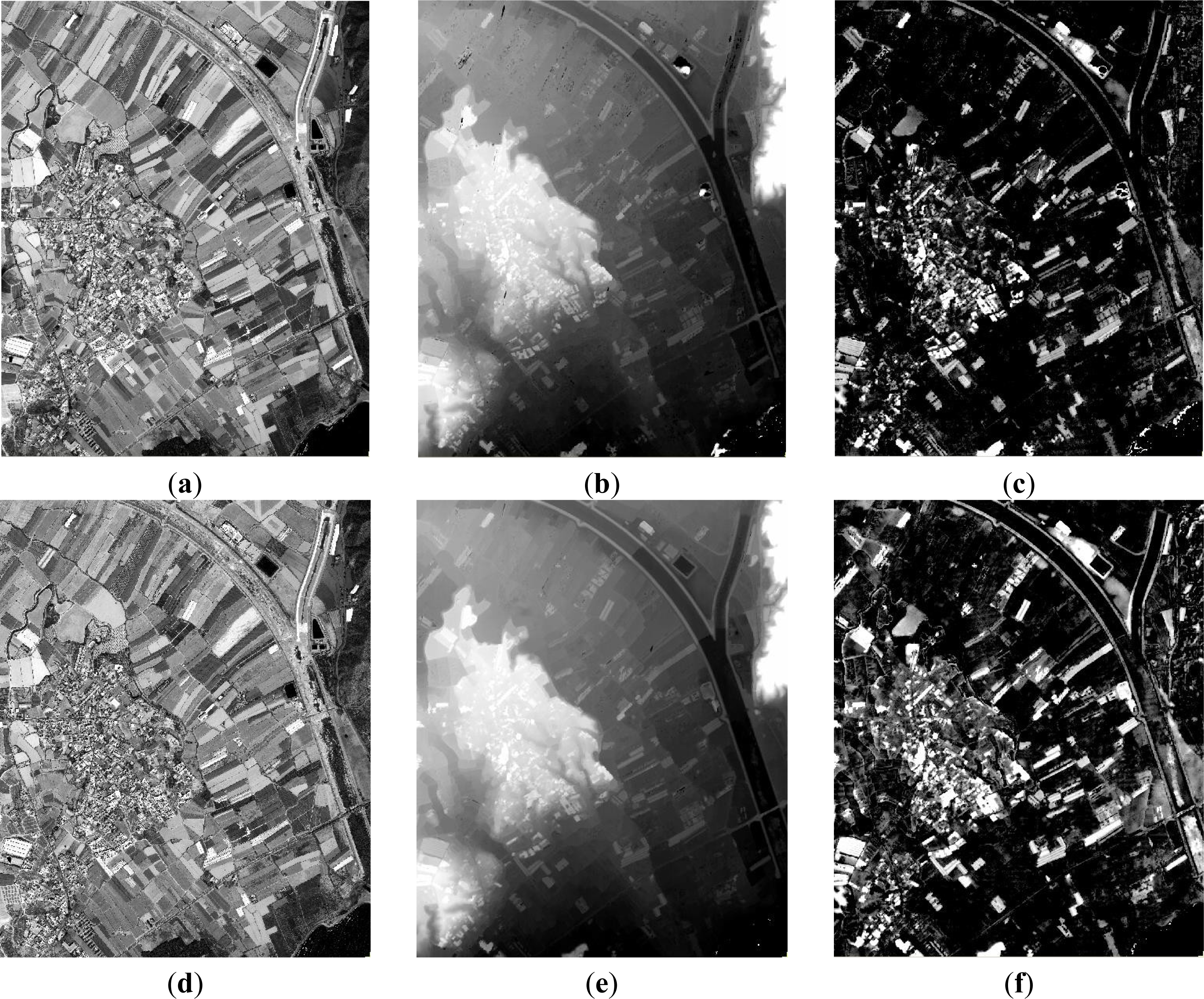
From the WV2 ORS2A stereo pair, two PAN orthoimages (one from the 22.4° off-nadir image (WV22) and the second from the 10° off-nadir one (WV10; see Figure 2a)) were generated by using the Andalusia DEM as ancillary data. Seven ground control points (GCPs) were always used to compute the sensor model based on rational functions refined by a zero order transformation in the image space (RPC0). In the same way, two pan-sharpened orthoimages were also generated from the corresponding images, WV10 and WV22 (with 0.5 m GSD and containing the spectral information gathered from the 8-band MS image) by applying the PANSHARP algorithm included in Geomatica 2013 (PCI Geomatics, Richmond Hill, ON, Canada). Both PAN and pan-sharpened orthoimages were made up of 4690 × 5800 pixels. The planimetric accuracies (RMSE_2D) computed on the orthorectified PAN and pan-sharpened images were 0.56 m and 0.86 m for WV10 and WV22 respectively (see the work recently published by Aguilar et al. [38] for more information about the orthorectification process).

A 1-m grid spacing DSM covering the whole study area was extracted from the WV2 PAN stereo pair by means of the photogrammetric software package, OrthoEngine, also included in Geomatica 2013 (Figure 2b). It is noteworthy that any editing process was applied to the DSMs compiled from VHR satellite imagery in order to keep their production as hands-off as possible. The corresponding DSM vertical accuracy, measured as standard deviation, was ranging from 0.53 m over flat areas to 2.74 m over urban areas [34]. A normalized digital surface model (nDSM) with 1-m grid spacing was calculated by subtracting the Andalusia DEM from the WV2-derived DSM (Figure 2c).

From the GE1 stereo pair and following the same procedure applied to WV2, two PAN and two 4-band pan-sharpened orthoimages (from the images with 23.1° (GE23) and 8.5° (GE9) off-nadir) were produced by using the Andalusia DEM, seven GCPs and the RPC0 sensor model. The RMSE_2D estimated over the PAN and pan-sharpened orthoimages were 0.48 m and 0.66 m for GE9 and GE23, respectively [38]. Figure 2d shows the corresponding PAN orthoimage from GE9 image. As in the case of WV2, an nDSM (Figure 2f) was computed by subtracting the Andalusia DEM from the GE1 PAN stereo pair DSM (Figure 2e). The standard deviation of this GE1-derived DSM ranged from 0.39 m over flat areas to 2.67 m over urban areas [34].

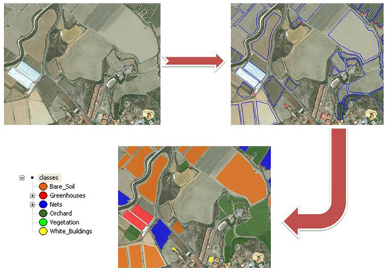
A flowchart is depicted in Figure 3 in order to clarify the pre-processing methodology carried out to generate both orthoimages and nDSMs data sets from VHR satellite stereo pairs.

3.2. Manual Segmentation and Reference Map

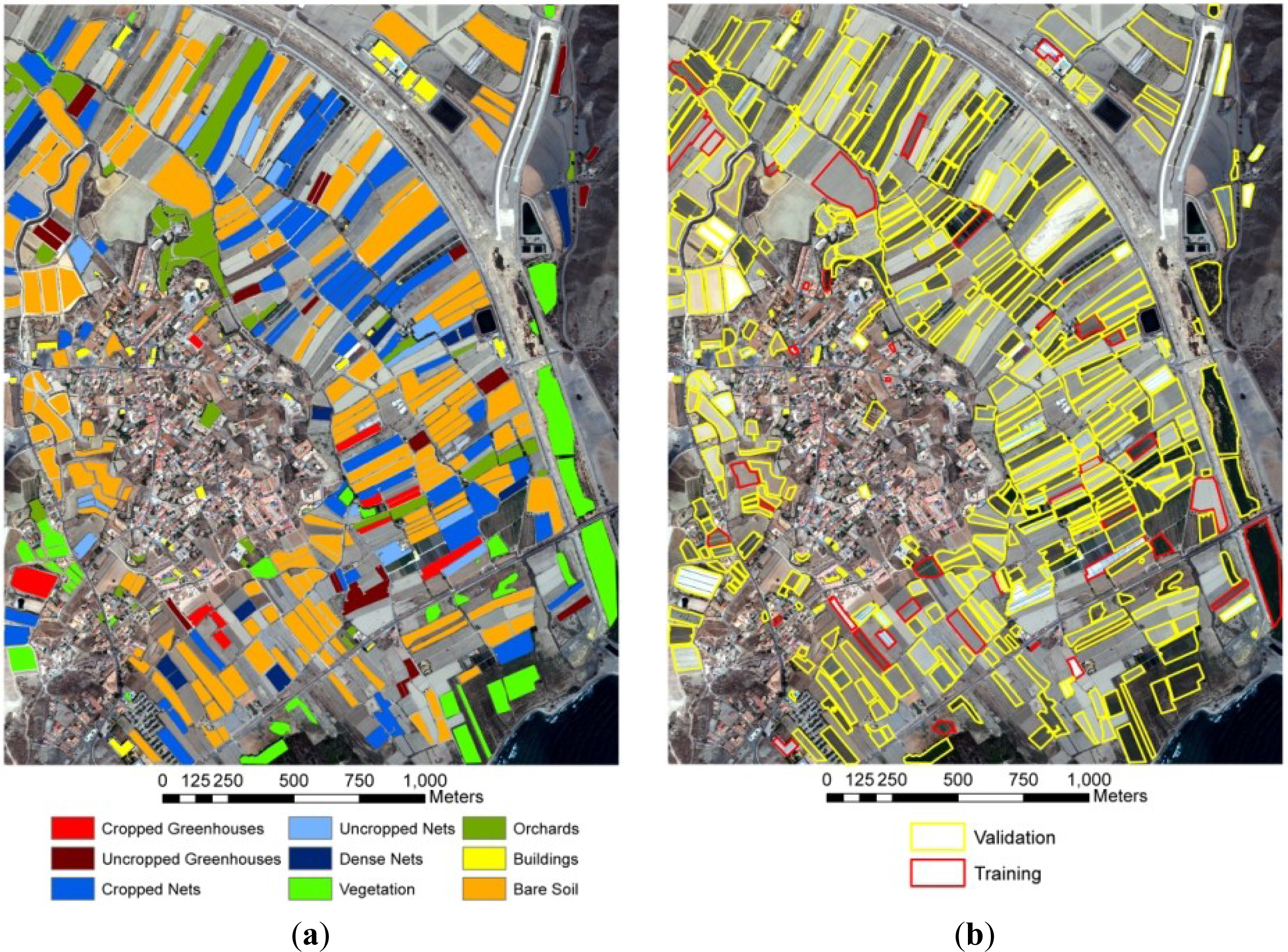
The first step in OBIA consists of image segmentation to produce homogeneous and discrete regions, objects or segments, which will be used later as the classification units instead of pixels [24,39]. VHR satellite imagery segmentation is a crucial step for attaining high accuracies at the final OBIA classification [40,41]. Anyway, generating segmentations from a multiangle data set (two different off-nadir viewing angle orthoimages from each stereo pair in our case) presents a unique set of challenges related to the geometric changes of elevated objects projections (e.g., buildings or greenhouses) depending on the different off-nadir angles (perspective view). For that reason, it is necessary to undertake an individual segmentation for each image belonging to the same stereo pair. However, this turns out to be excessively time consuming, and the OBIA classification from all multiangle images would be much more complex, as the objects created from one image do not fully match those coming from the other. Besides, the use of individual segmentations for orthoimages of GE1 and WV2 would hamper the direct comparison between both sensors. Hence, only a single manual segmentation of the study area was conducted, and it was used for all orthoimages. The 406 objects making up this segmentation were generated by manual digitizing performed over the PNOA’s aerial orthoimage at an approximate scale of 1:500 (Figure 4). These digitized objects always belonged to the nine classes shown in Figure 4a.

Cropped greenhouses and uncropped greenhouses included the plastic-covered greenhouses according to whether or not they were housing horticultural crops when the satellite images were taken. Cropped nets and uncropped nets were comprised of mesh-covered greenhouses with or without horticultural crops underneath. Dense nets could be defined as greenhouses covered by a green thick mesh material. The building class consisted of white buildings ranging from small sheds to large industrial buildings. Finally, the last three considered classes were vegetation, orchards and bare soil. Since our main goal was focused on greenhouse classification, both with plastic film and shadow mesh, all greenhouses present in the study area were digitized and assigned to classes cropped greenhouses, uncropped greenhouses, cropped nets, uncropped nets and dense nets. Since in some cases, the spectral differences between cropped and uncropped greenhouses covered by either plastic or mesh material were small (mainly depending on the type and the stage of development of the crop underneath), it was decided to group all these classes in only greenhouses and nets (

Table 2. Characteristics of WV2 and GE1 stereo pairs acquired at the study site.

Considered Classes	Final Classes	Training Objects	Validation Objects	Total
Cropped Greenhouses	Greenhouses	3	8	11
Uncropped Greenhouses		3	19	22
Cropped Nets	Nets	4	60	64
Uncropped Nets		4	12	16
Dense Nets		3	8	11
Vegetation	Vegetation	6	36	42
Orchards	Orchards	4	38	42
White Buildings	Buildings	9	44	53
Bare Soil	Bare Soil	6	139	145

). It should be borne in mind that the ground-truth or reference map was only based on the orthoimages from PNOA, GE1 and WV2, as well as very valuable information retrieved from the Google Street View tool (i.e., there was no field campaign in August 2011).

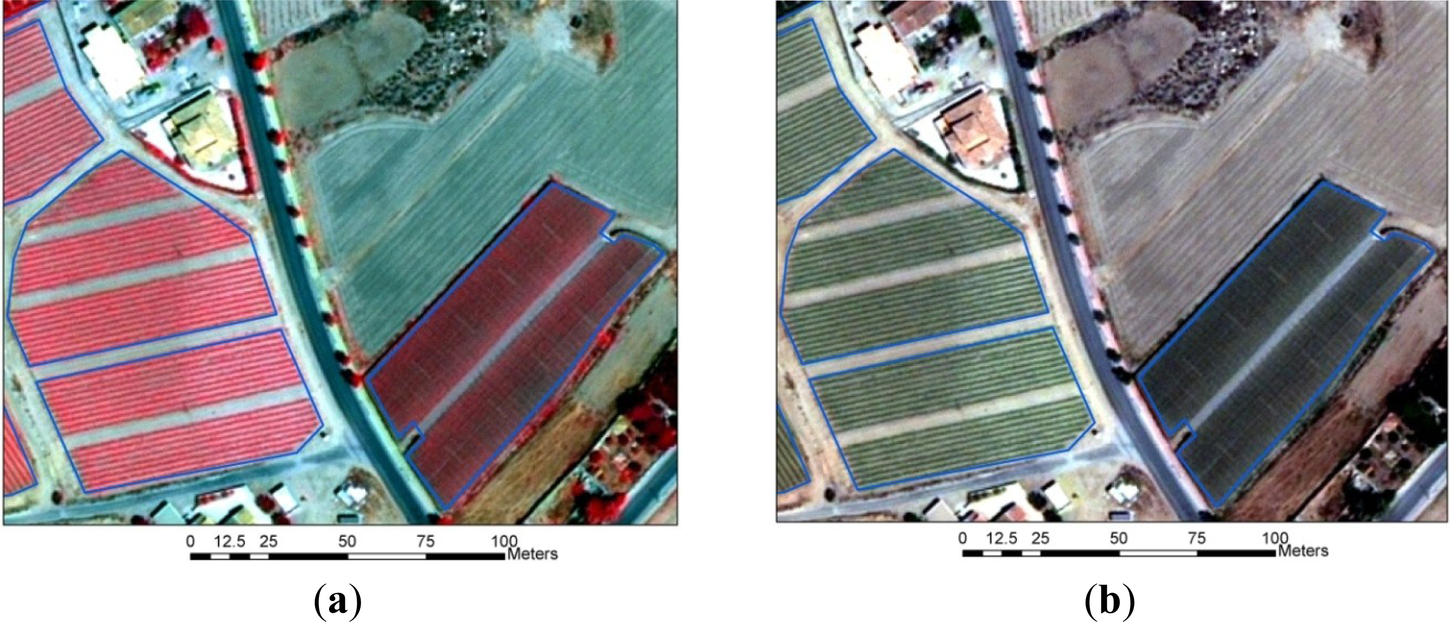
The classes, vegetation, orchards, bare soil and buildings, were selected for their spectral similarity to greenhouses and nets (Table 2). According to Van der Wel [10], the class, greenhouses (referring to plastic greenhouses), could be confused with white buildings. In the same way, Sanjuan [13] reported problems discriminating between nets (greenhouses covered with shadow meshes) and bare soil. Furthermore, cropped net greenhouses with leafy and overgrown crops underneath could be confused with vegetation, as can be seen in Figure 5, where an outdoor lettuce crop can be appreciated on the left-hand side of the road, while on the right, a cropped net greenhouse can be distinguished. The six final classes selected in this work are very similar to the ones chosen by Tarantino and Figorito [9], although they did not consider white buildings.

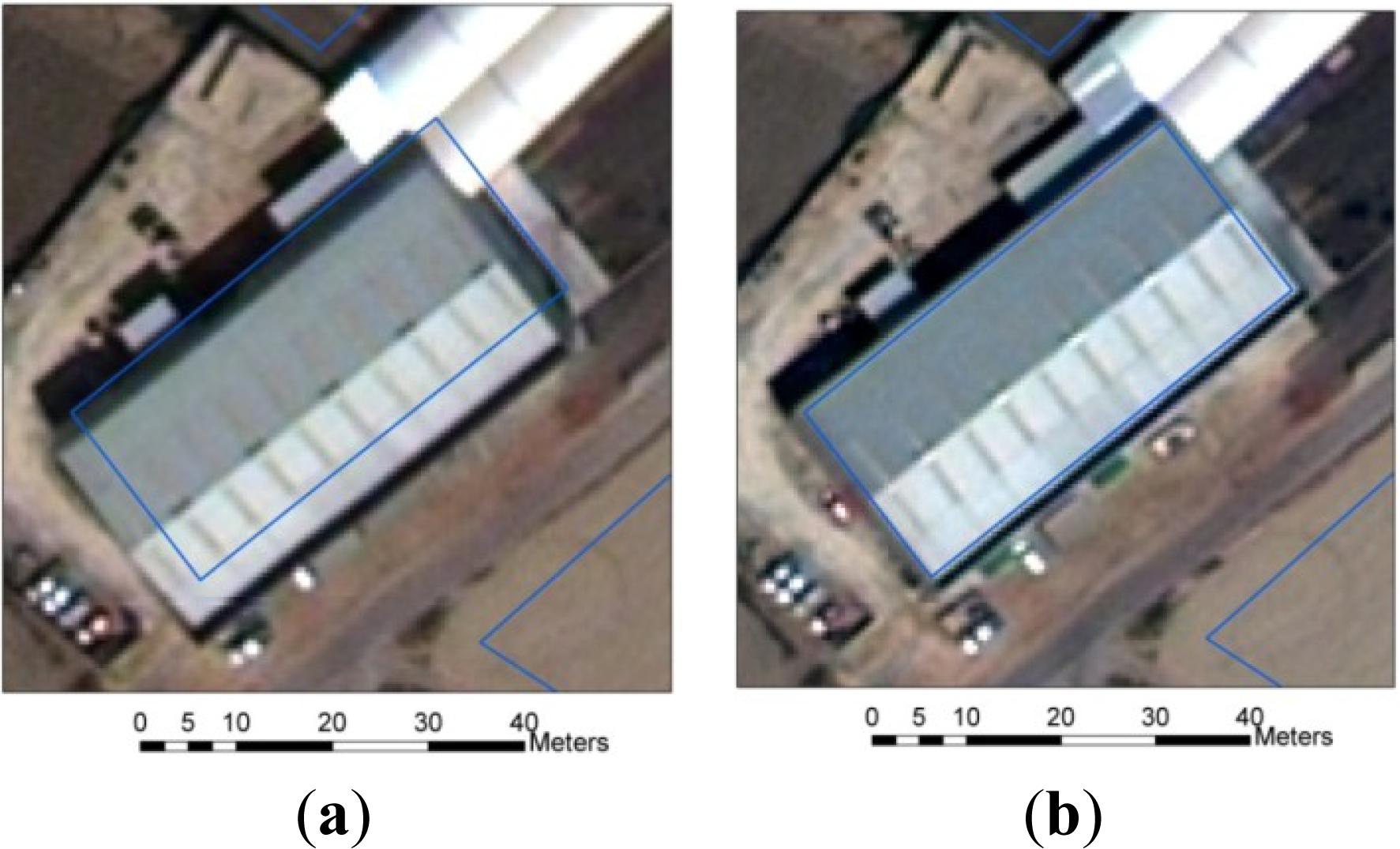
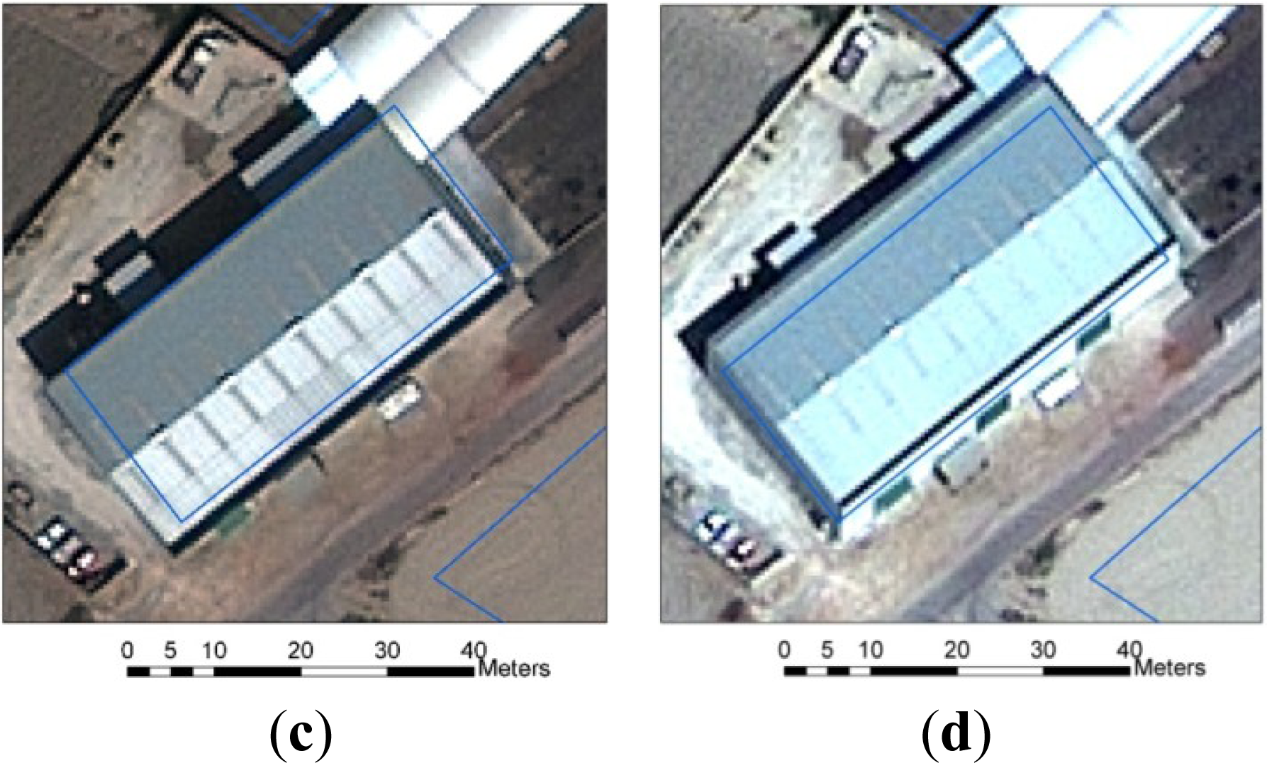
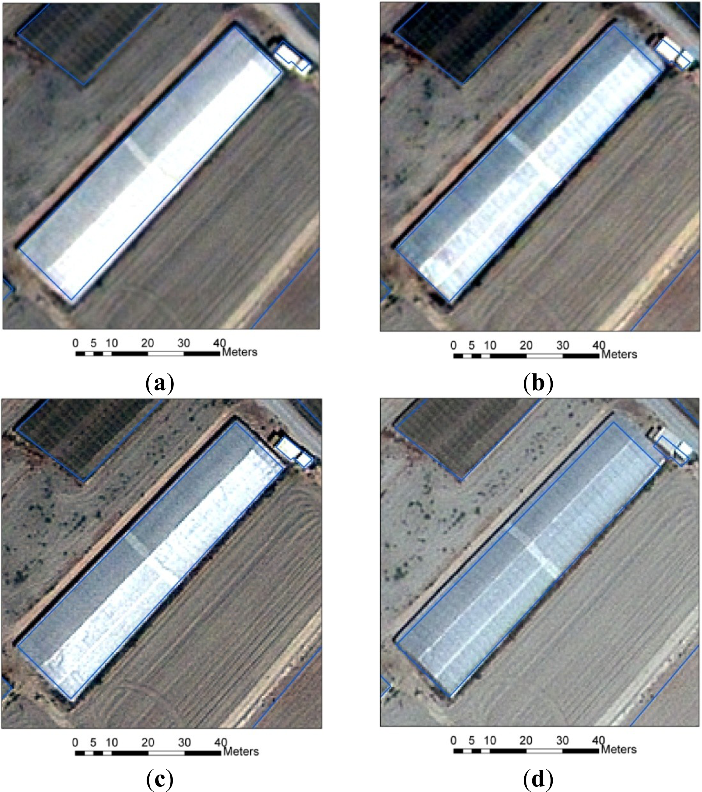
Figures 6 and 7 show an industrial building of about 9 m high and a very similar 4-m high plastic greenhouse over the four pan-sharpened orthoimages. It is noted that the objects digitized over the PNOA’s orthoimage (blue line) do not always match well the object boundaries, which can be made out on satellite orthoimagery, due to different off-nadir view angles. This effect is even more noticeable in the objects with higher height and smaller area (see the little building digitized on the northwest corner of Figure 7).

3.3. Classification Procedure

The OBIA software used in this research was eCognition 8.0. Once the manual segmentation with 406 objects has been transferred to eCognition by using a previously digitized vector file as a thematic layer, it comes time to tackle the classification phase. A very well-known classifier, like nearest neighbor (NN), which is included in eCognition, was applied in this work. NN is a non-parametric supervised classifier, which stands out because of its simplicity and flexibility.

A subset of 42 well-distributed objects (approximately 10% of the 406 previously digitized objects) was selected to carry out the training phase, whereas the remaining 364 objects, also evenly distributed on the working area, were used for the validation phase (Figure 4b). In a similar work, Tarantino and Figorito [9] used 30 training samples to train the eCognition’s NN classifier. Moreover, Aguilar et al. [20] reported that, in statistical terms, the most efficient choice dealing with urban areas classification from VHR imagery would be about 10% of training samples. In our case, the distribution among classes of both subsets is shown in Table 2. The NN classification was initially undertaken on the nine classes depicted in Table 2, but the final results were computed based on the final six classes by simply aggregating the classes corresponding to greenhouses and nets.

The object features selected to perform the supervised classification are presented and described in

Table 3. Image object features based on basic spectral information and band indices used in the classification phase. The NIR band of GE1 is expressed as NIR1.

	Tested Features	Applied to	Description
Basic Spectral Information	Brightness_4	Both	Overall intensity for classical bands (R, G, B and NIR1)
	Brightness_8	Only WV2	Overall intensity for 8-band of WV2
	Coastal	Only WV2	Mean, standard deviation and ratio to scene of coastal band
	Blue	Both	Mean, standard deviation and ratio to scene of blue band
	Green	Both	Mean, standard deviation and ratio to scene of green band
	Yellow	Only WV2	Mean, standard deviation and ratio to scene of yellow band
	Red	Both	Mean, standard deviation and ratio to scene of red band
	Red Edge	Only WV2	Mean, standard deviation and ratio to scene of red edge band
	NIR1	Both	Mean, standard deviation and ratio to scene of NIR1 band
	NIR2	Only WV2	Mean, standard deviation and ratio to scene of NIR2 band
	nDSM	Both	Mean, standard deviation and ratio to scene of nDSM band
Band Indices	NDBI	Both	Normalized difference of blue band index, (mean NIR1 − mean blue)/(mean NIR1 + mean blue)
	NDGI	Both	Normalized difference of green band index, (mean NIR1 − mean green)/(mean NIR1 + mean green)
	NDVI	Both	Normalized Difference Vegetation Index, (mean NIR1 − mean red)/(mean NIR1 + mean red)
	NDBI_NIR2	Only WV2	Normalized difference of blue band index using NIR2, (mean NIR2 − mean blue)/(mean NIR2 + mean blue)
	NDGI_NIR2	Only WV2	Normalized difference of green band index using NIR2, (mean NIR2 − mean green)/(mean NIR2 + mean green)
	NDVI_NIR2	Only WV2	Normalized Difference Vegetation Index using NIR2, (mean NIR2 − mean red)/(mean NIR2 + mean red)
	NDYI_NIR2	Only WV2	Normalized difference of yellow band index using NIR2, (mean NIR2 − mean yellow)/(mean NIR2 + mean yellow)
Band Indices	NDREI_NIR2	Only WV2	Normalized difference of red edge band index using NIR2, (mean NIR2 − mean red edge)/(mean NIR2 + mean red edge)
	NDCI_NIR2	Only WV2	Normalized difference of coastal band index using NIR2, (mean NIR2 − mean coastal)/(mean NIR2 + mean coastal)
	CRI	Only WV2	Carotenoid reflectance, (1/mean green) − (1/mean red edge)
	EVI	Only WV2	Enhanced vegetation index, 2.5 × (mean NIR2 − mean red)/(mean NIR2 + 6 × mean red – 7.5 × mean blue + 1)
	VOGRE	Only WV2	Vogelmann red edge 1, mean red edge/mean red

and

Table 4. Image object features based on texture, shape and geometry used in the classification phase. More information about these features can be found in [42]. GLCM, gray-level co-occurrence matrix.

	Tested features	Applied to	Description
Texture	GLCMcon	Both	GLCM contrast sum of all directions from PAN
	GLCMcon	WV2-8b	GLCM contrast sum of all directions from NIR1 and NIR2
	GLCMent	Both	GLCM entropy sum of all directions from PAN
	GLCMent	WV2-8b	GLCM entropy sum of all directions from NIR1 and NIR2
	GLCMmean	Both	GLCM mean sum of all directions from PAN
	GLCMmean	WV2-8b	GLCM mean sum of all directions from NIR1 and NIR2
	GLCMstdv	Both	GLCM standard deviation sum of all directions from PAN
	GLCMstdv	WV2-8b	GLCM std. dev. sum of all directions from NIR1 and NIR2
	GLCMcor	Both	GLCM correlation sum of all directions from PAN
	GLCMcor	WV2-8b	GLCM correl. sum of all directions from NIR1 and NIR2
Shape and Geometry	Area	Both	The number of pixels within an image object
	Roundness	Both	How similar an image object is to an ellipse
	Rectangular fit	Both	How well an image object fits into a rectangle
	Shape index	Both	The border length of the objects divided by four times the square root of its area
	Compactness	Both	The ratio of the area of a polygon to the area of a circle with the same perimeter
	Border index	Both	The number of edges that form the polygon
	Density	Both	The density is calculated by the number of pixels forming the image object divided by its approximated radius

. More in-depth information about these features can be found in the Reference Book of Definiens eCognition Developer 8 [42]. CRI, EVI and VOGRE in Table 3 are vegetation indices used by Oumar and Mutanga [43].

In the case of GE1, three different tests were carried out. The first of them was based on the GE9 PAN and pan-sharpened orthoimages (Single GE9). The second one used the GE23 PAN and pan-sharpened orthoimages (Single GE23). Finally, the third test considered all the information included in the two first cases, i.e., it used features from GE9 and GE23 orthoimages (stereo GE1).

Moreover, the features from image objects were grouped into 10 strategies for classification:

(1)

Super basic (SB): This set only includes the mean values of B, G, R and NIR bands. It has 4 features for both single GE9 and single GE23 and, therefore, 8 features for stereo GE1.

(2)

Super basic and elevation (SB + nDSM): It is composed of the SB’s features and the mean and standard deviation values computed from the nDSM within every object. It counts on 6 features for both single GE9 and single GE23, and 10 features for stereo GE1 (notice that the mean and standard deviation values coming from the nDSM have the same value for both single images).

(3)

Basic (B): This set includes the mean and standard deviation values computed from the B, G, R and NIR bands. Therefore, it accounts for 8 features for both single GE9 and Single GE23 and 16 features for stereo GE1.

(4)

Basic and band indices (B + BIs): This strategy is composed of the B’s features and the three normalized difference indices (NDBI (Normalized Difference Blue Index), NDGI (Normalized Difference Green Index) and NDVI). It adds up 11 features for both single GE9 and single GE23 and 22 features for stereo GE1.

(5)

Basic and ratios to scene (B + Rs): This set includes the B strategy plus four ratios to scene for R, G, B and NIR. It has 12 features for both single GE9 and single GE23 and 24 features for stereo GE1.

(6)

Basic and nDSM (B + nDSM): It is composed of the B’s features and the mean and standard deviation values computed from the nDSM. It has 10 features for both single GE9 and single GE23 and 18 features for stereo GE1 (note that the mean and standard deviation values from nDSM are the same for both single images).

(7)

Basic plus shape and geometry (B + Sh): It is composed of the B’s features plus the seven features corresponding to shape and geometry (Table 4). It has 15 features for both single GE9 and single GE23 and 23 features for stereo GE1 (note that the seven features related to shape and geometry present the same value for both single images).

(8)

Basic and texture (B + T): This set includes the B strategy plus five gray-level co-occurrence matrix (GLCMs) texture measurements computed on a PAN orthoimage. Only five out of the 14 GLCM texture features originally proposed by Haralick et al. [44] are considered in this work, due to both the strong correlation frequently reported between many of them [45] and their large computational burden. The same subset of GLCM texture features (i.e., contrast, entropy, mean, standard deviation and correlation) was selected by Stumpf and Kerle [46] working on a similar OBIA workflow. Therefore, the B + T set has 13 features for both single GE9 and single GE23 and 26 features for stereo GE1.

(9)

Basic plus nDSM and band indices (B + BIs + nDSM): This set includes the features corresponding to B + BIs and B + nDSM strategies. It has 13 features for both single GE9 and single GE23 and 24 features for stereo GE1 (the mean and standard deviation values from nDSM are the same for both single images).

(10)

All features (All): This strategy is composed of the sum of the following groups of features: (i) mean, standard deviation and ratio to scene for R, G, B, NIR and nDSM; (ii) Brightness_4; (iii) NDBI, NDGI and NDVI; (iv) 7 shape and geometry features; and (v) 5 texture features. Thus, it has 31 features for both single GE9 and single GE23 and 51 features for stereo GE1. In the case of stereo GE1, the features from nDSM and, shape and geometry are the same for both single images. Moreover, brightness is computed for each object as the mean value of the 8 bands involved (i.e., 4 RGBNIR bands from each image making up the stereo pair).

In the case of WV2, six different tests were conducted. On the one hand, three of them were carried out by only using the four classical bands included in WV2 MS imagery, i.e., R, G, B and NIR1 (it is noted that the NIR1 band in WV2 would correspond to the NIR band in GE1). In those cases, the information corresponding to the newest bands (i.e., coastal, yellow, red edge and NIR2) was not considered. These first three tests were undertaken in exactly the same way as single GE9, single GE23 and stereo GE1, and again, the same aforementioned 10 strategies for GE1 classification were applied. These tests were named as: (i) single WV10-4, based on WV10 orthoimages, but only using four bands; (ii) single WV22-4, using 4-band WV22 orthoimages; and (iii) stereo WV2-4, using 4-band orthoimages from both WV10 and WV22. On the other hand, the last three tests were conducted by using the complete 8 bands included in the MS WV2 imagery, and they were named single VW10-8, single WV-22-8 and stereo WV2-8.

Once again, 10 strategies for classification were applied in a similar way to GE1 or WV2 4-band cases. They were the following:

(1)

SB: 8 features for both single WV10-8 and single WV22-8 and 16 features for stereo WV2-8.

(2)

SB + nDSM: 10 features for the single tests and 18 features for stereo WV2-8.

(3)

B: 16 features for the single tests and 32 features for stereo WV2-8.

(4)

B + BIs: 22 features for the single tests, i.e., using 6 band indices, such as NDBI_NIR2, NDGI_NIR2, NDVI_NIR2, NDYI_NIR2, NDREI_NIR2 and NDCI_NIR2, and so, 44 features for stereo WV2-8.

(5)

B + Rs: 24 features for the single tests and 48 features for stereo WV2-8.

(6)

B + nDSM: 18 features for the single tests and 34 features for stereo WV2-8.

(7)

B + Sh: 23 features for the single tests and 39 features for stereo WV2-8.

(8)

B + T: 26 features for the single tests, i.e., using 10 GLCMs from NIR1 and NIR2, as recommended by Pu and Landry [47], and 52 features for stereo WV2-8.

(9)

B + BIs + nDSM: 24 features for the single tests and 46 features for stereo WV2-8.

(10)

All features: 57 features are used for the single tests (i.e., single VW10-8 and single WV-22-8), including mean, standard deviation and ratio to scene for WV2 8-band and nDSM, plus Brightness_8, plus 12 band indices, plus 7 shape and geometry features and plus 10 texture features. In the case of stereo WV2-8, 103 features are considered.

The number of features and strategies used in the classification stage are summarized in

Table 5. Number of features used in the classification stage for each strategy and test. SB, super basic; BI, band index; Sh, shape and geometry; Rs, ratio to scene; T, texture.

Test	Strategy
	1 SB	2 SB + nDSM	3 B	4 B + BIs	5 B + Rs	6 B + nDSM	7 B + Sh	8 B + T	9 B + BIs + nDSM	10 All
Single GE9	4	6	8	11	12	10	15	13	13	31
Single GE23	4	6	8	11	12	10	15	13	13	31
Stereo GE1	8	10	16	22	24	18	23	26	24	51
Single WV10-4	4	6	8	11	12	10	15	13	13	31
Single WV22-4	4	6	8	11	12	10	15	13	13	31
Stereo WV2-4	8	10	16	22	24	18	23	26	24	51
Single WV10-8	8	10	16	22	24	18	23	26	24	57
Single WV22-8	8	10	16	22	24	18	23	26	24	57
Stereo WV2-8	16	18	32	44	48	34	39	52	46	103

for a better understanding for the reader.

Regarding non-parametric supervised classification methods, comparative studies have shown that classification accuracy obtained from more sophisticated methods, such as support vector machines (SVM), may outperform NN [48–50]. Besides, SVM usually turns out to be more stable in high-dimensional feature spaces needing a small training sample size [51,52]. However the SVM model’s classification accuracy is largely dependent on the selection of the model’s parameters [53]. In short, SVM methods try to find a hyperplane that splits a data set into two subsets during the training phase [54]. Preliminarily, the input features are mapped into a higher-dimensional space through a suitable kernel function to obtain that hyperplane. Herein, we used a radial basis kernel function (RBF) and estimated the kernel parameter (γ) and the penalty parameter (C) through cross-validation from the training data [53]. The free-distribution library, LIBSVM [53], was employed for applying the SVM classifier to the aforementioned 9 tests (i.e., single GE9, single GE23, stereo GE1, single WV10-4, single WV22-4, stereo WV2-4, single WV10-8, single WV22-8 and stereo WV2-8), but only using the strategy named All features, which presents the most high-dimensional feature space.

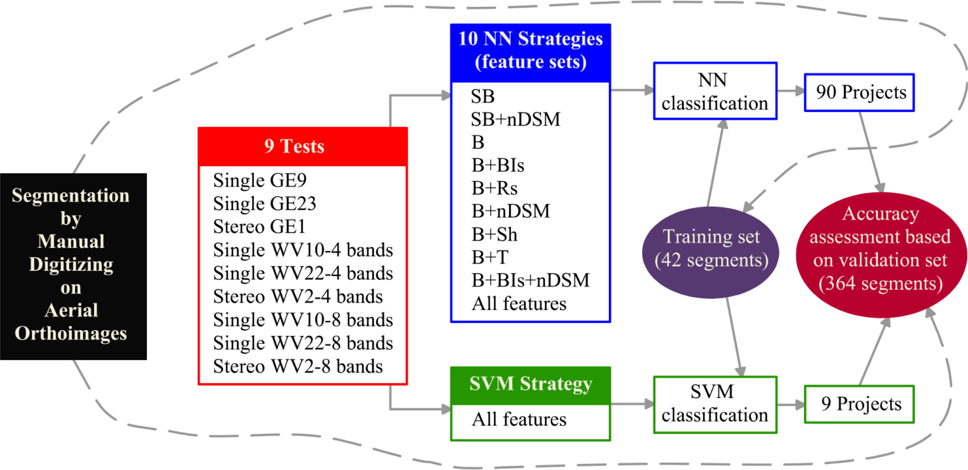
Taking into account the complex experimental design accomplished in this work, a synthetic flowchart is presented in Figure 8 in order to clarify the classification procedure section.

3.4. Accuracy Assessment

Summing up, 9 tests and 10 different strategies (i.e., 90 classification projects) were conducted in this work by applying the NN algorithm. Furthermore, the SVM classifier was tested for the 9 tests, but only for the strategy named All features (i.e., 9 classification projects). All the classifications tasks carried out in this study were performed over the same training objects (42), and the corresponding accuracies were always assessed against the same testing objects (364).

The classification accuracy assessment undertaken in this work was based on the error matrix [55]. Hence, the accuracy measures, always computed on the same validation set, were the following: user’s accuracy (UA), producer’s accuracy (PA) and overall accuracy (OA).

Finally, the F_β measure [19,56], which provides a way of combining UA and PA into a single measure, was also computed according to the Equation (1), where the parameter, β, determines the weight given to the user’s and producer’s accuracies. The value used in this study (β = 1) weighs UA equal to PA.

$$F_{\beta }=\frac{\left({\beta }^2+1\right)\times \text{PA}\times \text{UA}}{{\beta }^2\times \text{PA}+\text{UA}}$$

(1)

4. Results and Discussion

4.1. Classification Accuracy with Regard to the Strategies

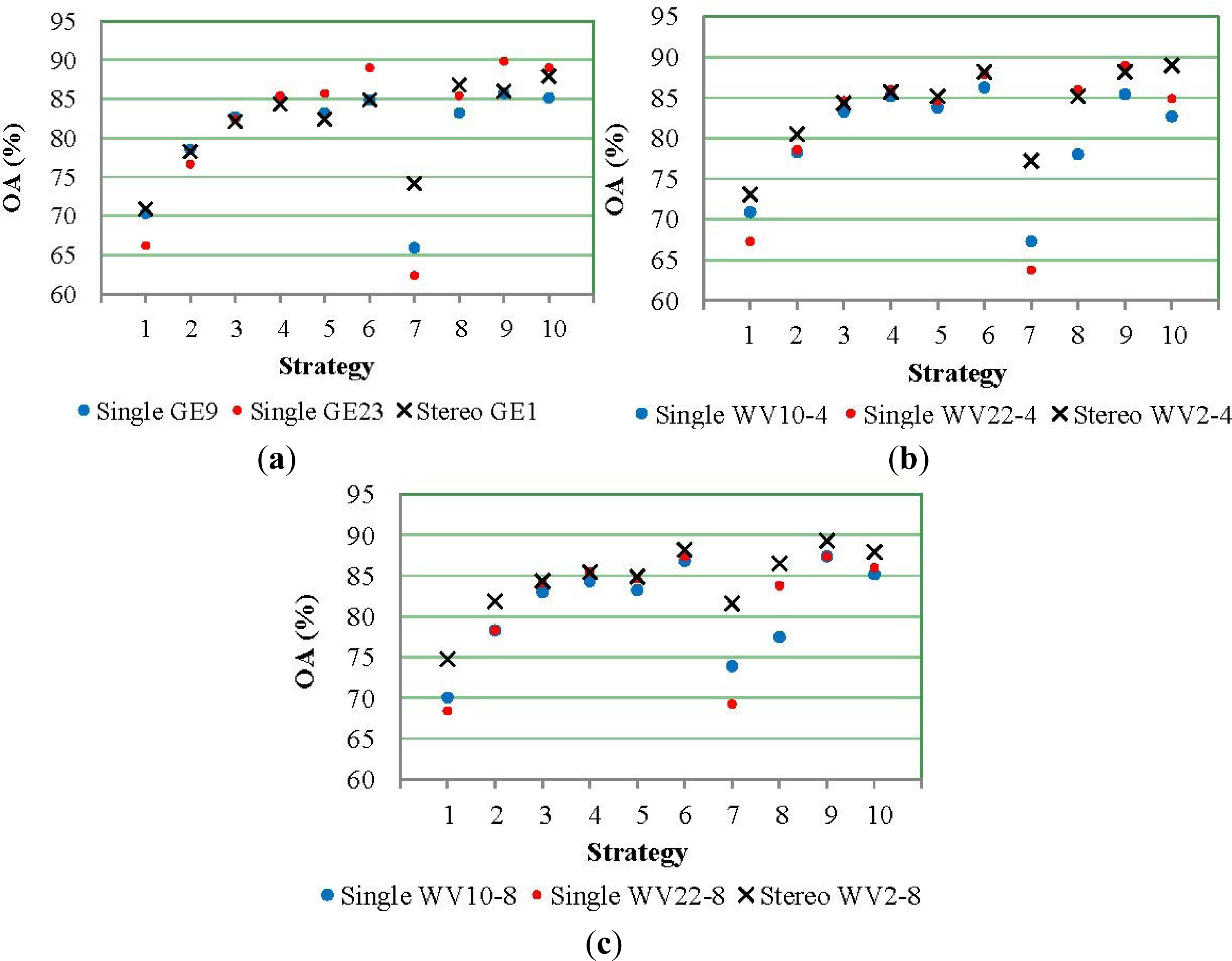
The obtained land cover classification results from using different tests and strategies, but always applying the NN algorithm included in eCognition, are depicted in Figure 9.

The overall accuracies values attained from GE1 projects (Figure 9a), WV2 using only the four classical bands (Figure 9b) and WV2 using all eight bands (Figure 9c), showed similar behavior. Regarding the strategies tested along this work, and as a general rule, B + nDSM (Strategy 6), B + BIs + nDSM (Strategy 9) and All features (Strategy 10) outperformed the others. Both BIs (mainly NDVI, NDBI and NDGI) and especially nDSM added valuable information to the basic spectral data represented here by the strategy, SB (Strategy 1, where only spectral band mean values are considered) and B (Strategy 3, where mean and standard deviations are included). In fact, the average OA of the nine tests was improved by approximately 3.6 percentage points when nDSM information was added to the B strategy, while a much more modest increase of 1.8% was attained by using BIs features. The importance of height data in the classification results can also be quantified by observing the large difference in overall accuracy (close to 9%) between the attained results in SB and SB + nDSM strategies for all the considered tests. In this way, but working on an urban environment, an improvement of 13% in the F-measure (F_β) was reported by Longbotham et al. [19] when height data compiled from a VHR stereo pair was added to the eight-band mean values of the single nadir pan-sharpened image of WV2. They achieved even larger increases when the target classes presented higher heights (e.g., skyscrapers or buildings).

Digital height maps have already been extracted from VHR stereo pairs for helping to the classify tasks. For example, Mahmoudi et al. [21] and Tian et al. [36] used a robust stereo matching algorithm based on semi-global matching (SGM) developed by Hirschmüller [57] on stereo pairs of IKONOS and WV2. Anther dense matching method, implemented in the BAE Systems’ Socket Set NGATE module, was used by Longbotham et al. [19] to extract DSM from WV2 multiangle images. A more conventional matching algorithm included in the OrthoEngine Module of PCI Geomatica was also used by Koc-San and Turker [35] over IKONOS stereo pairs. This last algorithm coincided with the matching algorithm applied in our work to attain the DSM. Although it usually performed quite well for both GE1 and WV2 stereo pairs, as can be seen in Figure 2b,e, it presented several problems working on greenhouses covered by shadow nets and also in urban areas (Figure 10). The last issue has been already reported by Aguilar et al. [34]. Just to give the reader an idea of the global behavior of the matching algorithm used in this work, Figure 11 shows the mean height of each object computed from GE1 nDSM with regard to its area (the results for WV2 turned out to be very similar). It can be noted that the objects belonging to plastic greenhouses presented a very homogeneous height around 4 m, indicating that the matching algorithm worked very well on this type of surface. In the case of greenhouses covered by shadow nets, the computed mean heights per object were much more heterogeneous, ranging from zero to 4 m. Finally, and dealing with buildings, problems due to an inaccurate nDSM were only evident when working with small objects. In fact, buildings presenting a size bigger than 2,000 pixels were assigned nDSM mean values ranging from 5.6 m to 11.3 m in the case of the GE1 stereo pair (from 4.9 m to 11.5 m in the case of WV2 stereo pair).

Regarding texture features, the second-order textural parameters tested in the Strategy 8 (B + T) did not clearly improve the results achieved by the B strategy. However, Longbotham et al. [19] achieved improvements higher than 10% by adding to the original spectral information several texture features calculated from the WV2 PAN band, such as homogeneity, contrast, dissimilarity, entropy, second moment and correlation. In our work, textural information seems to be totally covered by the standard deviation values of the spectral bands as a first-order texture measure.

Strategy 5 based on ratios to scene (B + Rs) hardly had any influence on the classification results. In addition, shape and geometry features included in Strategy 7 not only failed to improve overall accuracy values achieved in the B strategy, but they significantly worsened it.

4.2. Classification Accuracy with Regard to the Tests

Considering that manual segmentation was performed on an aerial orthoimage, the digitized objects should geometrically match the nearest nadir satellite orthoimagery better than those with a larger off-nadir (see Figures 6 and 7). Thus, as for the tests that consider only single images, the classification accuracy should be better for projects based on orthoimages presenting the smallest off-nadir (i.e., single GE9, single WV10-4 and single WV10_8). However, disregarding the heterogeneous Strategy 7, this fact only occurred for the SB and SB + nDSM strategies. Focusing on the three best strategies (i.e., B + nDSM, B + BIs + nDSM and All features), OA values were always worse in the tests carried out with near-nadir orthoimages, especially in the case of GE1. For instance, using the B + nDSM strategy as a reference, OA values of 89.01% and 84.89% were attained for single GE23 and single GE9, respectively. In the WV2 tests, OA values of 87.91% and 86.26% were computed for single WV22-4 and single WV10-4, while 87.39% and 86.81% were achieved for single WV22-8 and single WV10-8, respectively. In an attempt to understand these unexpected results, the per-class accuracy is shown for the three main strategies in Figure 12. It can be noted that the OA improvements corresponding to the tests with the higher off-nadir orthoimages were mainly due to a better effective discrimination between greenhouses and buildings classes and, so, increasing the F_β measure in both classes. In fact, misclassification between these two classes often occurred in small buildings, which were finally classified as greenhouses. In this way, Figure 13 shows the classification results of a detailed area inside our study area, where the existing seven small buildings are highlighted in red (Figure 13b). Four and three out of seven buildings were misclassified in single GE9 (Figure 13c) and single WV10-8 (Figure 13d), respectively. Bearing in mind that the displacements of the roof of the small buildings due to changes in off-nadir are rather variable (see the small building located in the upper right corner, Figure 7), the features computed for these small objects in each test also become very heterogeneous. In our work, and due to this edge effect, it seems that the small buildings in the tests presenting a high off-nadir offered unique spectral characteristics, and this fact improved the discrimination between greenhouses and buildings classes. However, this effect strongly depends on several factors, such as the segmentation process, the sun and satellite position and the elevation at the time of the image collection. Anyway, confusion between small buildings and greenhouses can be easily solved in operational conditions by introducing a threshold condition involving the area of these objects. A similar procedure was conducted by Agüera et al. [7] and Arcidiacono and Porto [58].

Regarding the classification results coming from adding multiangle orthoimages spectral information (i.e., stereo GE1, stereo WV2-4 and stereo WV2-8), no significant improvement with respect to the single tests was achieved. Furthermore, OA from stereo GE1 were worse than single GE23 for the best three strategies. In general, OA from stereo tests achieved the best results when the strategy All features was used. In the last case, the per-class accuracies measured as F_β (Figure 12) were much more homogeneous for each of the six classes (F_β values lower than 80%). So far, and to the best knowledge of the authors, multiangle satellite images had been used by Longbotham et al. [19] and Duca and Del Frate [37] for the generation of land cover maps. However, the last works were carried out by using pixel-based classification schemes, so they did not have to face the problem of segmentation, which is vital in an OBIA approach.

Another novel contribution of this paper was the comparison between the performance of newly developed VHR satellite imagery from WV2 and GE1 to classify land cover in mainly intensive agricultural environments with emphasis on greenhouse detection. Looking at Figure 12, any clear difference can be observed in the classification accuracy achieved for both GE1 and WV2-4 tests. Moreover, the new spectral bands of WV2 could not provide a significant improvement, neither in OA nor in per-class accuracy. Regarding the classes related to greenhouses (i.e., greenhouses and nets), they reached very acceptable F_β values ranging from 82% to 95% for any single test involving GE23 or WV22 orthoimages. According to Marchisio et al. [59], the use of the eight-band WV2 yielded improvements in classification accuracy figures ranging from 5% to 20% for certain land-cover types, such as man-made materials, selected vegetation targets, soils and shadows. In fact, Pu and Landry [47] compared VHR imagery from IKONOS and WV2 to identify and map urban forest tree species, finding that the 8-band WV2 significantly increased the accuracy of identifying tree species with respect to IKONOS data. In the same way, Koc-San [22] reported that using all 8 bands of WV2 satellite imagery was important to differentiate glass and plastic greenhouses. By contrast, Aguilar et al. [20] did not find improvements in classification accuracy between GE1 and WV2 imagery when working on urban environments, whereas Marshall et al. [60] concluded that there was no benefit in using the additional four bands of WV2 to discriminate invasive grass species.

Finally, the best OA values achieved in this work by using OBIA techniques on a very heterogeneous greenhouse area were close to 90% for both GE1 and WV2 cases. As it was mentioned before in the introduction section, few papers can be found in the literature related to greenhouse detection by using different pixel-based approaches. Although Agüera et al. [7] reported a greenhouse detection percentage value of 91.45% working with QuickBird images, it was achieved after applying two algorithms to refine the raw classification (both to eliminate loops and to define the sides of greenhouses). The same authors [5] compared QuickBird and IKONOS imagery in plastic greenhouse detection and analyzed the effect of texture in the pixel-based classification accuracy. They concluded that the addition of texture information in the classification process did not improve the classification accuracy, and the best results in terms of greenhouse detection percentage took values of 89.61% and 88.26% for QuickBird and IKONOS, respectively. Working on WV2 pan-sharpened imagery, Koc-San [22] reported OA values from 87.80% to 93.88% by using different pixel-based classification techniques, such as maximum likelihood, random forest and SVM. Arcidiacono and Porto [15] reported a greenhouse detection percentage of 85.71% by using RGB VHR satellite bands only. This accuracy was improved to 88.42% by adding texture descriptors. In the same way, Arcidiacono and Porto [28] compared both pixel and object-based approaches to classify greenhouses on RGB aerial images. The best accuracy results ranging from 83.15% to 94.73% were attained by using OBIA techniques (in this case, the commercial software, VLS Feature Analyst^® for Leica Erdas Imagine^®). Last, but not least, Tarantino and Figorito [9] achieved an OA of 90.25% by using OBIA classification implemented in eCognition for mapping plastic-covered vineyards from aerial photographs.

In summary, a lot of approaches (mainly grouped into pixel-based and OBIA techniques) have already been applied to greenhouse detection on VHR aerial or satellite imagery. However, the classification accuracy always was around 90%. Taking into account that the study areas in the aforementioned works were very changeable, it is difficult to properly compare these results. In this sense, it is important to consider the differences in the cost of each type of imagery and also the specialized software needed to perform each approach.

4.3. Classification Accuracy with Regard to the Classifier

Classifications algorithms frequently used in object-based approaches, as is the case of NN, do not perform well on a high-dimensional feature space, due to problems related to feature correlation (the widely known curse of dimensionality). In this section, the SVM classifier, which had previously shown a good performance in dealing with large number of features [49], was compared to the NN classifier for all features strategy (i.e., nine tests). Although OA values were very similar for NN and SVM classifiers, they were always slightly better when NN was applied.

Table 6. PA and UA per class attained for each stereo test by using the NN or SVM classifier and the all features strategy.

NN and SVM Multiangle Tests	Stereo GE1				Stereo WV2_4				Stereo WV2_8
	NN		SVM		NN		SVM		NN		SVM
	PA (%)	UA (%)	PA (%)	UA (%)	PA (%)	UA (%)	PA (%)	UA (%)	PA (%)	UA (%)	PA (%)	UA (%)
Greenhouses	100	79.4	92.6	89.3	100	87.1	85.2	100	92.6	83.3	81.5	91.7
Nets	97.5	78	90	75.8	97.5	83.9	90	78.3	100	80.8	96.3	81.1
Vegetation	75	90	77.8	68.3	77.8	82.4	72.2	61.9	77.8	84.8	83.3	75
Orchards	89.5	87.2	65.8	75.8	89.5	79.1	55.3	61.8	84.2	82.1	71.1	87.1
Buildings	70.5	100	90.9	93	75	100	93.2	93.2	72.7	94.1	90.9	87
Bare Soil	88.5	98.4	87.8	98.4	89.2	98.4	88.5	95.3	88.5	97.6	87.8	95.3
Overall Accuracy (%)	87.91		85.71		89.01		84.07		87.91		87.36

shows the accuracy results in terms of PA and UA measures, but only for the stereo tests, which presented the most high-dimensional feature space. For each row, the bold values highlight the best accuracies for both PA and UA, respectively. On the whole, NN performed quite well with bare soil, greenhouses and nets, whereas SVM only outperformed NN in the case of the buildings class.

The misclassification between vegetation and net classes (mainly with cropped shadow nets), which had been very significant when using Strategies 6 and 9 (Figure 12), seems to have decreased when the All features strategy was used with NN. However, the performance of SVM when classifying vegetation and orchards was quite poor.

5. Conclusions

This work compares the capabilities of stereo pairs from GE1 and WV2 VHR satellite imagery for land cover classification with emphasis on detecting greenhouses covered by plastic films or shadow nets. To this end, features based on spectral information coming from both PAN and pan-sharpened orthoimages and a digital height map extracted by stereo matching from satellite imagery were used together through an OBIA approach. As far as we know, this is the first work to use single-source height and multispectral information coming from both images of each stereo pair (i.e., multiangle orthoimages) for the purpose of greenhouse classification.

The study was implemented in an agricultural area around the village of Palomares, Almería (Spain). Likely, the study site counted on a very low number of greenhouses, especially those covered by plastic film. Furthermore, these greenhouses were very heterogeneous, both in terms of type of covering and the crop underneath.

The segmentation process was carried out by manually digitizing on aerial orthoimages. In this way, the digitized objects could be used for all the tests conducted in this work, involving orthoimages with different off-nadir from both WV2 and GE1. In further practical applications, and working with the two multiangle images of one stereo pair by using OBIA techniques, the segmentation step could be automatically performed on the most vertical or near-nadir orthoimage. Furthermore, thematic vector layers might be also used if they were available.

The overall accuracies attained by the NN classifier from GE1 tests (four MS bands) turned out to be very similar to the ones computed from WV2 (either four or eight MS bands) for every set of features tested. In general, nDSM was the most important feature for greenhouse classification. In fact, the three best strategies (i.e., B + nDSM, B + BIs + nDSM and all features) included height data extracted from the VHR stereo pair. The best overall accuracy values were close to 90%, and they were not improved by the use of multiangle orthoimages (stereo tests). The shape and geometric features (B + Sh), ratios to scene (B + Rs) and texture features based on GLCM (B + T) did not contribute to improving the classification attained by the basic spectral features strategy (B).

Disaggregating the results by class, the behavior of the three single tests performed with the near-nadir orthoimages (i.e., single GE9, single WV10-4 and single WV10-8) became very similar when applying the three best strategies. In these tests, there were a lot of misclassification problems between greenhouses and buildings classes, presenting F_β indices usually lower than 75%. In fact, many small buildings were misclassified as plastic greenhouses. Curiously, this problem was partially solved in the single tests using the higher off-nadir orthoimages, due to the significant displacements of the roofs of the small buildings. In this way, these small objects, including pixels from other land cover in their edges, presented unique characteristics that helped for their correct classification. Anyway, and regarding an operational case, confusion between small buildings and greenhouses can be easily solved considering the area of these objects (i.e., introducing a threshold condition). More difficult to solve would be the misclassification between vegetation and nets (when the last are cropped), especially taking into account that the DSM extracted over mesh greenhouses was not very accurate.

Finally, NN and SVM non-parametric classifiers were compared through the All features strategy. The theoretical superiority of the SVM approach, as compared to NN, was not confirmed in this study. In fact, OA values were always slightly better when NN was applied.

Further works should be focused on testing new dense matching algorithms to improve the DSM extraction, especially on greenhouses with mesh covering and urban areas. Furthermore, the accuracy of the automatic segmentation process applied to the greenhouse area poses a great challenge. We are now planning to address both topics in new Mediterranean study sites mainly dedicated to greenhouse growing.

References

- Espi, E.; Salmeron, A.; Fontecha, A.; García, Y.; Real, A.I. Plastic films for agricultural applications. J. Plast. Film Sheeting 2006, 22, 85–102. [Google Scholar]
- Levin, N.; Lugassi, R.; Ramon, U.; Braun, O.; Ben-Dor, E. Remote sensing as a tool for monitoring plasticulture in agricultural landscapes. Int. J. Remote Sens 2007, 28, 183–202. [Google Scholar]
- Parra, S.; Aguilar, F.J.; Calatrava, J. Decision modelling for environmental protection: The contingent valuation method applied to greenhouse waste management. Biosyst. Eng 2008, 99, 469–477. [Google Scholar]
- Arcidiacono, C.; Porto, S. A model to manage crop-shelter spatial development by multi-temporal coverage analysis and spatial indicators. Biosyst. Eng 2010, 107, 107–122. [Google Scholar]
- Agüera, F.; Aguilar, F.J.; Aguilar, M.A. Using texture analysis to improve per-pixel classification of very high resolution images for mapping plastic greenhouses. ISPRS J. Photogramm. Remote Sens 2008, 63, 635–646. [Google Scholar]
- Picuno, P.; Tortora, A.; Capobianco, R.L. Analysis of plasticulture landscapes in Southern Italy through remote sensing and solid modelling techniques. Landsc. Urban Plan 2011, 100, 45–56. [Google Scholar]
- Agüera, F.; Aguilar, M.A.; Aguilar, F.J. Detecting greenhouse changes from QB imagery on the Mediterranean Coast. Int. J. Remote Sens 2006, 27, 4751–4767. [Google Scholar]
- Liu, J.G.; Mason, P. Essential Image Processing and GIS for Remote Sensing; Wiley: Hoboken, NJ, USA, 2009. [Google Scholar]
- Tarantino, E.; Figorito, B. Mapping rural areas with widespread plastic covered vineyards using true color aerial data. Remote Sens 2012, 4, 1913–1928. [Google Scholar]
- Van der Wel, F.J.M. Assessment and Visualisation of Uncertainty in Remote Sensing Land Cover Classifications. Ph.D. Thesis. Utrecht University, Utrecht, The Netherlands, 2000. [Google Scholar]
- Mesev, V.; Gorte, B.; Longley, P.A. Modified Maximum-Likelihood Classification Algorithms and Their Application to Urban Remote Sensing. In Remote Sensing and Urban Analysis; Donnay, J.-P., Barnsley, M.J., Longley, P.A., Eds.; Taylor & Francis: New York, NY, USA, 2000; pp. 62–83. [Google Scholar]
- Zhao, G.; Li, J.; Li, T.; Yue, Y.; Warner, T. Utilizing landsat TM imagery to map greenhouses in Qingzhou, Shandong Province, China. Pedosphere 2004, 14, 363–369. [Google Scholar]
- Sanjuan, J.F. Estudio Multitemporal Sobre la Evolución de la Superficie Invernada en la Provincia de Almería por Términos Municipales Desde 1984 Hasta 2004: Mediante Teledetección de Imágenes Thematic Mapper de los Satélites Landsat V y VII; Cuadrado, I.M., Ed.; Fundación para la Investigación Agraria de la Provincia de Almería: Almería, Spain, 2004. [Google Scholar]
- Carvajal, F.; Agüera, F.; Aguilar, F.J.; Aguilar, M.A. Relationship between atmospheric correction and training site strategy with respect to accuracy of greenhouse detection process from very high resolution imagery. Int. J. Remote Sens 2010, 31, 2977–2994. [Google Scholar]
- Arcidiacono, C.; Porto, S.M.C. Improving per-pixel classification of crop-shelter coverage by texture analyses of high-resolution satellite panchromatic images. J. Agric. Eng 2011, 4, 9–16. [Google Scholar]
- Arcidiacono, C.; Porto, S.M.C. Pixel-based classification of high-resolution satellite images for crop-shelter coverage recognition. Acta Hortic 2012, 937, 1003–1010. [Google Scholar]
- Arcidiacono, C.; Porto, S.M.C.; Cascone, G. Accuracy of crop-shelter thematic maps: A case study of maps obtained by spectral and textural classification of high-resolution satellite images. J. Food Agric. Environ 2012, 10, 1071–1074. [Google Scholar]
- Hussain, E.; Ural, S.; Kim, K.; Fu, C.; Shan, J. Building extraction and rubble mapping for city port-au-prince post-2010 earthquake with GeoEye-1 imagery and lidar data. Photogramm. Eng. Remote Sens 2011, 77, 1011–1023. [Google Scholar]
- Longbotham, N.; Chaapel, C.; Bleiler, L.; Padwick, C.; Emery, W.J.; Pacifici, F. Very high resolution multiangle urban classification analysis. IEEE Trans. Geosci. Remote Sens 2012, 50, 1155–1170. [Google Scholar]
- Aguilar, M.A.; Saldaña, M.M.; Aguilar, F.J. GeoEye-1 and WorldView-2 pansharpened imagery for object-based classification in urban environments. Int. J. Remote Sens 2013, 34, 2583–2606. [Google Scholar]
- Mahmoudi, F.T.; Samadzadegan, F.; Reinartz, P. Object oriented image analysis based on multi-agent recognition system. Comput. Geosci 2013, 54, 219–230. [Google Scholar]
- Koc-San, D. Evaluation of different classification techniques for the detection of glass and plastic greenhouses from WorldView-2 satellite imagery. J. Appl. Remote Sens 2013, 7. [Google Scholar] [CrossRef]
- Pohl, C.; van Genderen, J.L. Review article Multisensor image fusion in remote sensing: Concepts, methods and applications. Int. J. Remote Sens 1998, 19, 823–854. [Google Scholar]
- Blaschke, T. Object based image analysis for remote sensing. ISPRS J. Photogramm. Remote Sens 2010, 65, 2–16. [Google Scholar]
- Lu, D.; Hetrick, S.; Moran, E. Land cover classification in a complex urban-rural landscape with QuickBird imagery. Photogramm. Eng. Remote Sens 2010, 76, 1159–1168. [Google Scholar]
- Myint, S.W.; Gober, P.; Brazel, A.; Grossman-Clarke, S.; Weng, Q. Per-pixel vs. object-based classification of urban land cover extraction using high spatial resolution imagery. Remote Sens. Environ 2011, 115, 1145–1161. [Google Scholar]
- Weng, Q. Remote sensing of impervious surfaces in the urban areas: Requirements, methods, and trends. Remote Sens. Environ 2012, 117, 34–49. [Google Scholar]
- Arcidiacono, C.; Porto, S.M.C. Classification of crop-shelter coverage by RGB aerial images: A compendium of experiences and findings. J. Agric. Eng 2010, 3, 1–11. [Google Scholar]
- Haala, N.; Brenner, C. Extraction of buildings and trees in urban environments. ISPRS J. Photogramm. Remote Sens 1999, 54, 130–137. [Google Scholar]
- Hermosilla, T.; Ruiz, L.A.; Recio, J.A.; Estornell, J. Evaluation of automatic building detection approaches combining high resolution images and LiDAR data. Remote Sens 2011, 3, 1188–1210. [Google Scholar]
- Awrangjeb, M.; Ravanbakhsh, M.; Fraser, C.S. Automatic detection of residential buildings using LiDAR data and multispectral imagery. ISPRS J. Photogramm. Remote Sens 2010, 65, 457–467. [Google Scholar]
- Hobi, M.L.; Ginzler, C. Accuracy assessment of digital surface models based on WorldView-2 and ADS80 stereo remote sensing data. Remote Sens 2012, 4, 6347–6368. [Google Scholar]
- Poli, D.; Caravaggi, I. 3D modeling of large urban areas with stereo VHR satellite imagery: Lessons learned. Nat. Hazards 2013, 68, 53–78. [Google Scholar]
- Aguilar, M.A.; Saldaña, M.M.; Aguilar, F.J. Generation and quality assessment of stereo-extracted DSM from GeoEye-1 and WorldView-2 imagery. IEEE Trans. Geosci. Remote Sens 2014, 52, 1259–1271. [Google Scholar]
- Koc-San, D.; Turker, M. A model-based approach for automatic building database updating from high-resolution space imagery. Int. J. Remote Sens 2012, 33, 4193–4218. [Google Scholar]
- Tian, J.; Cui, S.; Reinartz, P. Building change detection based on satellite stereo imagery and digital surface models. IEEE Trans. Geosci. Remote Sens 2014, 52, 406–417. [Google Scholar]
- Duca, R.; Del Frate, F. Hyperspectral and multiangle CHRIS-PROBA images for the generation of land cover maps. IEEE Trans. Geosci. Remote Sens 2008, 46, 2857–2866. [Google Scholar]
- Aguilar, M.A.; Saldaña, M.M.; Aguilar, F.J. Assessing geometric accuracy of the orthorectification process from GeoEye-1 and WorldView-2 panchromatic images. Int. J. Appl. Earth Obs. Geoinf 2013, 21, 427–435. [Google Scholar]
- Carleer, A.P.; Wolff, E. Urban land cover multi-level region-based classification of VHR data by selecting relevant features. Int. J. Remote Sens 2006, 27, 1035–1051. [Google Scholar]
- Song, M.; Civco, D.; Hurd, J. A competitive pixel-object approach for land cover classification. Int. J. Remote Sens 2005, 26, 4981–4997. [Google Scholar]
- Liu, D.; Xia, F. Assessing object-based classification: advantages and limitations. Remote Sens. Lett 2010, 1, 187–194. [Google Scholar]
- Definiens eCognition. Definiens eCognition Developer 8 Reference Book; Definiens AG: München, Germany, 2009. [Google Scholar]
- Oumar, Z.; Mutanga, O. Using WorldView-2 bands and indices to predict bronze bug (Thaumastocoris peregrinus) damage in plantation forests. Int. J. Remote Sens 2013, 34, 2236–2249. [Google Scholar]
- Haralick, R.M.; Shanmugam, K.; Dinstein, I.H. Textural features for image classification. IEEE Trans. Syst. Man Cybern 1973, 3, 610–621. [Google Scholar]
- Baraldi, A.; Panniggiani, F. An investigation of the textural characteristics associated with gray level cooccurrence matrix statistical parameters. IEEE Trans. Geosci. Remote Sens 1995, 33, 293–304. [Google Scholar]
- Stumpf, A.; Kerle, N. Object-oriented mapping of landslides using random forests. Remote Sens. Environ 2011, 115, 2564–2577. [Google Scholar]
- Pu, R.; Landry, S. A comparative analysis of high spatial resolution IKONOS and WorldView-2 imagery for mapping urban tree species. Remote Sens. Environ 2012, 124, 516–533. [Google Scholar]
- Foody, G.M.; Mathur, A. A relative evaluation of multiclass image classification by support vector machines. IEEE Trans. Geosci. Remote Sens 2004, 42, 1335–1343. [Google Scholar]
- Melgani, F.; Bruzzone, L. Classification of hyperspectral remote sensing images with support vector machines. IEEE Trans. Geosci. Remote Sens 2004, 42, 1778–1790. [Google Scholar]
- Fernández, I.; Aguilar, F.J.; Álvarez, M.F.; Aguilar, M.A. Non-parametric object-based approaches to carry out ISA classification from archival aerial orthoimages. IEEE J. Sel. Top. Appl. Earth Obs. Remote Sens 2013, 6, 2058–2071. [Google Scholar]
- Foody, G.M.; Mathur, A. The use of small training sets containing mixed pixels for accurate hard image classification: Training on mixed spectral responses for classification by a SVM. Remote Sens. Environ 2006, 103, 179–189. [Google Scholar]
- Chen, C.H.; Ho, P.G.P. Statistical pattern recognition in remote sensing. Pattern Recognit 2008, 41, 2731–2741. [Google Scholar]
- Chang, C.C.; Lin, C.J. LIBSVM: A library for support vector machines. ACM Trans. Intell. Syst. Technol 2011, 2, 1–27. [Google Scholar]
- Vapnik, V.N. The Nature of Statistical Learning Theory; Springer-Verlag: NewYork, NY, USA, 1995. [Google Scholar]
- Congalton, R.G. A review of assessing the accuracy of classifications of remotely sensed data. Remote Sens. Environ 1991, 37, 35–46. [Google Scholar]
- Aksoy, S.; Akcay, H.G.; Wassenaar, T. Automatic mapping of linear woody vegetation features in agricultural landscapes using very high-resolution imagery. IEEE Trans. Geosci. Remote Sens 2010, 48, 511–522. [Google Scholar]
- Hirschmüller, H. Stereo processing by semiglobal matching and mutual information. IEEE Trans. Pattern Anal. Mach. Intell 2008, 30, 1–14. [Google Scholar]
- Arcidiacono, C.; Porto, S.M.C. Image processing for the classification of crop shelters. Acta Hortic 2008, 801, 309–316. [Google Scholar]
- Marchisio, G.; Pacifici, F.; Padwick, C. On the Relative Predictive Value of the New Spectral Bands in the WorldView-2 Sensor. Proceedings of the IEEE International Geoscience and Remote Sensing Symposium, Honolulu, HI, USA, 25–30 July 2010; pp. 2723–2726.
- Marshall, V.; Lewis, M.; Ostendorf, B. Do Additional Bands (Coastal, Nir-2, Red-Edge and Yellow) in WorldView-2 Multispectral Imagery Improve Discrimination of an Invasive Tussock, Buffel Grass (Cenchrus Ciliaris)? Proceedings of the International Archives of the Photogrammetry, Remote Sensing and Spatial Information Sciences (Vol. XXXIX-B8), XXII ISPRS Congress, Melbourne, Australia, 25 August–1 September 2012; pp. 277–281.