A Parallel Computing Paradigm for Pan-Sharpening Algorithms of Remotely Sensed Images on a Multi-Core Computer

Abstract

Pan-sharpening algorithms are data-and computation-intensive, and the processing performance can be poor if common serial processing techniques are adopted. This paper presents a parallel computing paradigm for pan-sharpening algorithms based on a generalized fusion model and parallel computing techniques. The developed modules, including eight typical pan-sharpening algorithms, show that the framework can be applied to implement most algorithms. The experiments demonstrate that if parallel strategies are adopted, in the best cases the fastest times required to finish the entire fusion operation (including disk input/output (I/O) and computation) are close to the time required to directly read and write the images without any computation. The parallel processing implemented on a workstation with two CPUs is able to perform these operations up to 13.9 times faster than serial execution. An algorithm in the framework is 32.6 times faster than the corresponding version in the ERDAS IMAGINE software. Additionally, no obvious differences in the fusion effects are observed between the fusion results of different implemented versions.

1. Introduction

Pan-sharpening is a process capable of integrating different images to produce a greater amount of information than can be derived from a single sensor [1]. Thus far, many pan-sharpening methods [2–8] have been presented in which the structural and textural details of the lower resolution multispectral image are enhanced by adopting the higher resolution panchromatic image corresponding to the multispectral image. Thus, the key issues of pan-sharpening concentrate on maximum enhancement of the spatial details at the expense of the minimum spectral distortion derived from the fusion operations. To achieve the stated goals, several sophisticated strategies (i.e., orthogonal transformation, filtering, wavelet transformation, Laplacian pyramid decomposition, regression, optimization, and numerical computing) are embodied in the fusion operations, which usually require reading and writing of a large amount of data. However, the implementation and use of these strategies lead to two obvious problems.

First, certain algorithms are quite difficult to implement, and the basic steps of each algorithm are not the same. The procedures for these algorithms are highly complicated and require many intermediate steps. For instance, the hybrid fusion algorithm [9] integrates the intensity-hue-saturation (IHS) and the principal component analysis (PCA) with multi-resolution analysis (MRA). Thus far, no general processing framework exists. A desirable framework would include basic steps corresponding to each fusion algorithm that are similar and can be applied to most fusion algorithms. Second, the immense computational cost of these algorithms is a realistic concern. The execution of these algorithms is notably slow if executed serially. For instance, a relatively simple algorithm (the Mod.IHS [10] Resolution Merge algorithm in the commercial software ERDAS IMAGINE) firstly transforms the multispectral image into IHS color space, then the matched panchromatic image replaces the intensity in IHS color space, lastly the fused image is transformed back into RGB color space. The algorithm is used to combine SPOT 5 panchromatic and multispectral images, it creates a 2.26-GB-sized file to save the fusion results. The whole procedure requires nearly 27 min to process on the latest workstation computer with a 3.06-GHz central processing unit (CPU). Normally, the entire process of serial execution for complicated algorithms is rather time-consuming.

However, the current computing resources are usually not utilized efficiently. The serial algorithm is unaware of the existence of multiple CPU cores, and the performance of such algorithm on a multi-core computer will be the same as its performance on a single core computer. The current serial algorithms are not matched to the development of computer hardware in which multi-core CPU is widely available. Hence, parallel computing methods are required that can fully leverage the state-of-the-art hardware platforms and can be easily adapted to pan-sharpening.

Fortunately, related studies have been published in the field of parallel processing for image sensing. Lee et al. [11] reviewed recent developments in high performance computing (HPC) for remote sensing. Achalakul and Taylor [12] described a concurrent spectral-screening principal component transform (PCT) algorithm employing low-cost, commercial-off-the-shelf multi-processors connected through high performance (gigabit) networking. Tehranian et al. [13] presented an architectural model and a system prototype for providing performance, reliability, and scalability of candidate hardware and software for a satellite data processing system. Plaza et al. [14,15] developed several highly innovative parallel algorithms for standard data processing and information extraction of hyperspectral images in heterogeneous networks of workstations and homogeneous clusters. Luo et al. [16] presented a parallel implementation of N-FINDR [17] (a widely used endmember extraction algorithm) in which the imagery is divided into multiple spatial partitions with entirely spectral pixels. Christophe et al. [18] compared the relative performance between a multithreaded program on CPU and the corresponding program running on graphic processing unit (GPU). Ma et al. [19,20] proposed a generic data-structure oriented programming template to support massive remote sensing data processing in high performance clusters. Wei et al. [21] presented a parallel framework that optimizes the parameter determination process for various algorithms of image fusion on Linux clusters. Parallel experiments based on multi-core processors, which mainly use the OpenMP (an API for shared-memory parallel programming), basic linear algebra subprograms (BLAS), and linear algebra package (LAPACK) libraries, can be found in the literature [22,23].

Although parallel strategies and parallel processing have been proposed in existing works, no parallel tests are available for pan-sharpening algorithms in a multi-core computer environment. We define the multi-core computer as a computer that contains single or multiple CPUs in one machine, with each CPU including multiple cores. Compared with the massive parallel processing (MPP) and cluster computers, the widely used multi-core computer possesses two important advantages. First, the multi-core computer is cheap and popular and therefore can be obtained easily by anyone, whereas large clusters or MPP computers are usually located in a supercomputing center with limited access. A multi-core computer can be managed and maintained more easily than a cluster or a MPP computer. Second, a multi-core computer contains enough CPU cores (or virtual cores) in a single machine with symmetrical multi-processing (SMP) or hyper-threading technology. For instance, the E5-2697 v2 CPU from the Intel Xeon E5 family is composed of 12 cores or 24 virtual cores using hyper-threading technology.

To resolve the existing problems, we present a parallel computing framework for pan-sharpening algorithms that relies primarily on two improvements. First, the implementation steps corresponding to each fusion algorithm are nearly identical in the proposed framework which can be applied to most pan-sharpening algorithms. Second, this framework is based on parallel computing; the adopted parallel strategies are able to fully leverage the computing resources of a multi-core computer. In this paper, eight typical pan-sharpening algorithms are implemented in the framework. The remainder of the paper is organized as follows. Section 2 shortly reviews the existing pan-sharpening algorithms and the fusion model. The proposed parallel computing framework is presented in Section 3, followed by the experiments and analysis in Section 4. Conclusions are presented in the Section 5.

2. A Short Overview of Existing Pan-Sharpening Algorithms

Typically, pan-sharpening algorithms can be divided into three general categories [24]: the component substitution (CS) fusion techniques, the modulation-based fusion techniques and the MRA-based fusion techniques. A recent review of these techniques is given in [24], and evaluation and comparison of selected fusion algorithms are presented in [25–32]. A higher level image fusion for remote sensing, i.e., feature fusion, can be found in [33].

In general, a CS-based fusion algorithm consists of three steps [2]. First, the original data are transformed into another data space via a forward transform, such as IHS transform or PCA transform. Next, a component of the transformed data is replaced by a higher resolution panchromatic image. Last, the replaced data are reversely transformed back to the original data space. The typical algorithms that apply the CS fusion techniques include IHS [2,34,35], PCA [2], Gram-Schmidt [36], and variants, such as generalized IHS (GIHS) [37], GIHS with tradeoff parameter (GIHS-TP) [38], GIHS with fixed weights (GIHS-F) [37], GIHS adaptive (GIHS-A) [39], improved adaptive IHS (IAIHS) [40], Gram–Schmidt Adaptive (GS-A) [39], fast spectral response function (FSRF) [41], CS with a histogram-matched panchromatic band, CS using sensor spectral response [42,43], CS for vegetation enhancement [44], and the FFT-enhanced IHS transform method [45].

The modulation-based fusion techniques use the following concept: the spatial details are modulated into the multispectral image by multiplying the multispectral image by the ratio of the panchromatic image to the synthetic image, which is a lower resolution version of the panchromatic image in general. The fusion results are expressed as Equation (1).

$${\mathit{xs}}_{\left(k,i,j\right)}^H=\frac{{\mathit{pan}}_{\left(i,j\right)}}{{\mathit{syn}}_{\left(i,j\right)}}{\mathit{xs}}_{\left(k,i,j\right)}^L$$

(1)

In Equation (1), xs^L_(k,i,j) and xs^H_(k,i,j) are the pixel values of the multispectral images before and after fusion, respectively, and pan_(i,j) is the pixel value of the panchromatic image, k is band number, (i, j) represents the pixel location and syn_(i,j) is the value of the (i, j) pixel of the synthetic band. The typical algorithms that apply the modulation-based fusion techniques include color normalization (CN) [46], smoothing filter based intensity modulation (SFIM) [4], synthetic variable ratio (SVR) [47], high pass filtering (HPF) [48], and local correlation modeling (LCM) [3].

The MRA-based fusion techniques adopt multi-resolution analysis methods, such as multi-resolution wavelet [5,49–53] and the Laplacian pyramid [54,55], to decompose multispectral and panchromatic images with different levels. They subsequently derive the spatial details that are imported into the finer scales of the multispectral images with respect to the relationship between the panchromatic and multispectral images in the coarser scales [5,54,56,57]. The typical fusion algorithms based on MRA include the à trous wavelet image fusion algorithm which adopts translation invariant and undecimated wavelet transform technique [50,58], and the fusion algorithm based on the generalized Laplacian pyramid (GLP) [54]. Some fusion algorithms use wavelet decomposition and CS jointly, such as the fusion algorithm combining wavelet decomposition with PCA [9,59,60] or IHS transform [9,61,62]. A Hybrid pan-sharpening algorithm combining Laplacian filtering and CS-based fusion can be found in [63]. Generally, these hybrid schemes use wavelet transforms to extract the spatial details from the panchromatic image and subsequently apply an orthogonal transform to inject the details into the multispectral image. The sensor spectral response and ground spectral features are introduced into the fusion techniques based on MRA in [43,64].

In addition, recently the numerical and optimization methods were designed to calculate the final fusion results according to the ideal imaging conditions and assessment criteria [65–71]. A statistical approach, University of New Brunswick (UNB)-pansharp, is presented in [72]. The newest efforts are to explore a sparse signal representation of image patches to solve the pan-sharpening problem [73,74].

Some presented algorithms can be described by a certain mathematical model. Shettigara [2] presented a generalized component substitution technique. The “Amélioration de la Résolution Spatiale par Injection de Structures” (ARSIS, improving spatial resolution by structure injection) concept is based on the assumption that the missing information is linked to the high frequencies of the datasets to be fused [5]. PCA, Brovey and wavelet transform fusion techniques are evaluated and found to be IHS-like image merging techniques [75]. A comprehensive framework, the general image fusion (GIF) method, makes it possible to categorize, compare, and evaluate the existing image fusion methods [76]. A generalized model can characterize most commonly used pan-sharpening algorithms [77]. Palubinskas [78] presented general fusion filtering framework (GFF), which is very suitable for a fusion of multi-resolution and multi-sensor data, as well as a simple and fast variant of GFF-high-pass filtering method. Inter-modality models in pan-sharpening are analyzed based on remote sensing physics in [79].

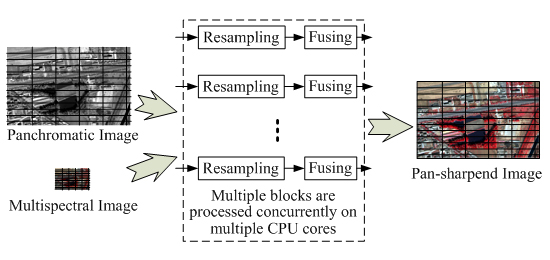
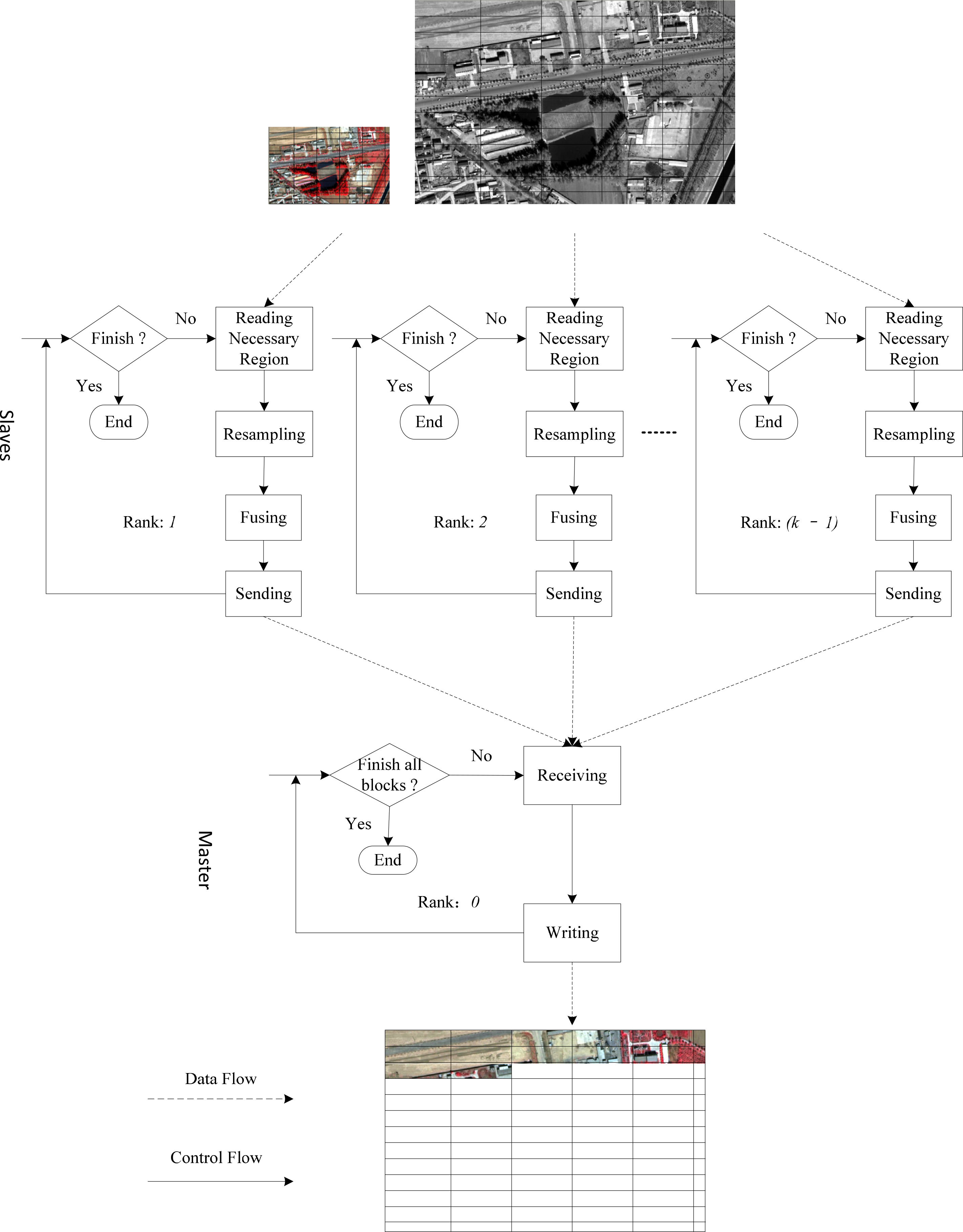
3. The Proposed Parallel Computing Framework

3.1. Direct Calculation of the Two Variables in the Generalized Model

In this paper the generalized model [77] is used. The generalized model for pan-sharpening is represented by the following formula:

$$x{s}_{\left(k,i,j\right)}^H=x{s}_{\left(k,i,j\right)}^L+{\alpha }_{\left(k,i,j\right)}\cdot {\delta }_{\left(i,j\right)}$$

(2)

where xs^L_(k,i,j) and xs^H_(k,i,j) are the pixel values before and after fusion, respectively, k is band number, (i, j) represents the pixel location, δ_(i,j) are the spatial details at (i, j) extracted from the higher resolution panchromatic image by a certain operation and α_(k,i,j) is the fusion coefficient (Injection Gain) used to modulate the detailed spatial δ_(i,j) into xs^L_(k,i,j).

In Equation (2), the spatial details extracted from the panchromatic band are injected into multispectral bands in terms of the fusion coefficients. The fusion results are the bands whose features are enhanced by the panchromatic image. When a specific algorithm is implemented using the framework, the first step is to transform the fusion algorithm into the generalized model and determine the expressions for calculating the two variables δ_(i,j) and α_(k,i,j) of the final fusion results, respectively. Different algorithms correspond to different calculation expressions of the two variables δ_(i,j) and α_(k,i,j). The main steps corresponding to each algorithm are nearly the same, i.e., calculation of the variables δ_(i,j) and α_(k,i,j). The typical algorithms selected from the three general categories in Section 2 were transformed into the generalized model in the study [80]. Zhang and Yang [80] list the calculation expressions of two important variables in the generalized model for commonly used algorithms. For the purpose of completeness, we recite the results from the literature [80] in

Table 1. Two important variables α_(k,i,j) and δ_(i,j) in the generalized model for most of the existing pan-sharpening algorithms [80].

Fusion Algorithm	α(k,i,j)	δ(i,j)
PCA	ωk1	pan(i,j)–pc1(i,j)
IHS	1	pan(i,j)–I(i,j)
RVS	ωk1	$$pa{n}_{(i,j)}-\left(c_1\cdot x{s}_{\left(1,i,j\right)}^L+c_2\cdot x{s}_{(2,i,j)}^L+c_3\cdot x{s}_{(3,i,j)}^L\right)$$
SFIM	$$\frac{x{s}_{\left(k,i,j\right)}^L}{sy{n}_{\left(i,j\right)}}$$	pan(i,j)− syn(i,j) where syn = f*pan
CN	$$\frac{3x{s}_{\left(k,i,j\right)}^L}{\sum _{k}x{s}_{\left(k,i,j\right)}^L}$$	$${\mathit{pan}}_{(i,j)}-\frac{1}{3}\left(x{s}_{(1,i,j)}^L+x{s}_{(2,i,j)}^L+x{s}_{(3,i,j)}^L\right)$$
à trous	Additive: 1 Minimum spectral distortion: $$\frac{x{s}_{(k,i,j)}^L}{{\mathit{pan}}_{A(i,j)}^2}$$	$${\mathit{pan}}_{(i,j)}-{\mathit{pan}}_{A(i,j)}^2$$ where $${\mathit{pan}}_A^1=f_1*\mathit{pan}$$ $${\mathit{pan}}_A^2=f_2*{\mathit{pan}}_A^1$$
GLP	Minimum spectral distortion: $$\frac{x{s}_{(k,i,j)}^L}{{\mathrm{pan}}_{p(i,j)}^L}$$ Context-based decision: $$\{\begin{array}{lll}\text{min}\left(\frac{{\sigma }_{(k,i,j)}^{xs}}{1+{\sigma }_{(i,j)}^{\mathit{pan}}},3\right),\hfill & \text{if}\hfill & {\rho }_{(k,i,j)}\ge {\theta }_k\hfill \\ 0,\hfill & \text{if}\hfill & {\rho }_{\text{(}k,i,j\text{)}}<{\theta }_k\hfill \end{array}$$	$${\mathit{pan}}_{(i,j)}-{\mathit{pan}}_{p(i,j)}^L$$ where $${\mathit{pan}}_p^L=e_p\left(\uparrow p\left(\downarrow p(r_p(\mathit{pan}))\right)\right)$$
Fusion algorithm combining wavelet decomposition with PCA transform	ωk1	$${\mathit{pan}}_{(i,j)}-{\mathit{pan}}_{A(i,j)}^2$$ where $${\mathit{pan}}_A^1=f_1*\mathit{pan}$$ $${\mathit{pan}}_A^2=f_2*{\mathit{pan}}_A^1$$
Fusion algorithm combining wavelet decomposition with IHS transform	1	$${\mathit{pan}}_{(i,j)}-{\mathit{pan}}_{A(i,j)}^2$$ where $${\mathit{pan}}_A^1=f_1*\mathit{pan}$$ $${\mathit{pan}}_A^2=f_2*{\mathit{pan}}_A^1$$
LCM	bk where $$x{s}_k^L=b_k\cdot {\mathit{pan}}^L+a_k+{\varepsilon }_k$$	$${\mathit{pan}}_{(i,j)}-{\mathit{pan}}_{(i,j)}^L$$ where panL is obtained by degrading pan
ARSIS	Context-based decision: $$\{\begin{array}{lll}\text{min}\left(\frac{{\sigma }_{(k,i,j)}^{xs}}{1+{\sigma }_{(i,j)}^{\mathit{pan}}},3\right),\hfill & \text{if}\hfill & {\rho }_{(k,i,j)}\ge {\theta }_k\hfill \\ 0,\hfill & \text{if}\hfill & {\rho }_{(k,i,j)}<{\theta }_k\hfill \end{array}$$ Ranchin-Wald-Mangolini model	$${\mathit{pan}}_{(i,j)}-{\mathit{pan}}_{\mathit{A}(i,j)}^n=\sum _n{\mathit{pan}}_{D(i,j)}^n$$ $${\mathit{pan}}_A^n$$ is an approximate component obtained by multi-resolution analysis for n levels. The methods for the multi-resolution analysis can be GLP, à trous wavelet transform and undecimated discrete wavelet transform (UDWT).
Block regression	$$\frac{x{s}_{(k,i,j)}^L}{\sum _k{c}_k\cdot x{s}_{(k,i,j)}^L}$$	pan(i,j) − syn(i,j), For each block: $$\mathit{syn}=c_1\cdot x{s}_1^L+c_2\cdot x{s}_2^L+c_3\cdot x{s}_3^L+c_4\cdot x{s}_4^L$$ $$\mathit{pan}=c_1\cdot x{s}_1^L+c_2\cdot x{s}_2^L+c_3\cdot x{s}_3^L+c_4\cdot x{s}_4^L+\delta$$

.

3.2. Block Partition

Direct calculation of the two variables can be fulfilled by means of blocks. As shown in Figure 1, the image file used to save the final fusion results (which has an image size that is usually the same as the panchromatic band) is partitioned into blocks. Next, the final fusion results in one block region are generated and written into the result file. In this paper, the tile partition whose size is 512 × 128 is adopted as a block partition. This parallel partition strategy is similar to those in the literature [12,14,81]; the only difference is that the tile partition in this paper is applied to computation as well as reading. However, the partition strategies in those are only applied to computation.

Not only the intensity value of the (i, j) pixels but also the global statistical information or neighbor pixels of location (i, j) are used for the location (i, j) in the course of calculation of δ_(i,j) and α_(k,i,j) in certain cases. Usually, three cases exist in which the necessary data are required to enable the entire processing of a block [81]. The case in which only the corresponding pixels are used and the case in which both the corresponding and neighboring pixels are used are shown in Figure 2a,b, respectively. The former includes the IHS, CN, and regression variable substitute (RVS) [2] approaches, and the latter includes the SFIM, à trous, LCM, and block regression methods [82]. The size of neighboring pixels in Figure 2b is determined by the fact that the necessary data are read to calculate the two variables. For the case in which the corresponding pixels and the global statistical information are used, the global information is generated prior to the parallel processing. PCA fusion method and the method combing PCA and à trous wavelet transform are two examples. Serial or parallel computing can be used to calculate global statistics according to the amount of required computation. In this paper, we adopt serial processing, because the time to calculate global statistics that is also included in the total time is a small portion of the total time. Section 4.1 gives the experimental results of the time for global statistics.

If several sub-steps are required to calculate the variables δ_(i,j) and α_(k,i,j), a recursive procedure for fetching and computation will be used in which each sub-step is the same as in the abovementioned cases. The two-level decomposition of the additive wavelet fusion is an example [50].

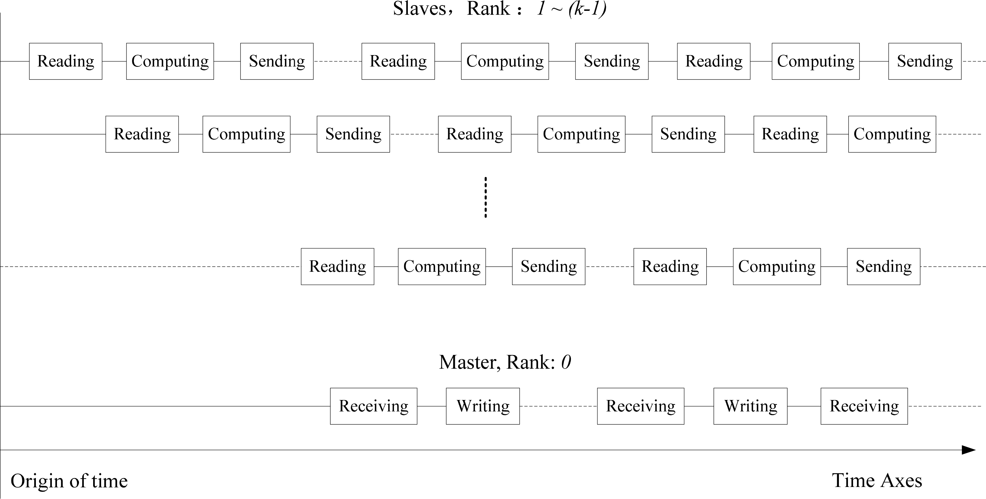
3.3. The Parallel Processing Mechanism

Because the fusion results can be generated and saved in the form of a block, the parallel computing approach can easily be incorporated into the framework. The parallel computing approach makes it possible for multiple blocks to be processed concurrently on multiple CPU cores. The message passing interface (MPI) is used as the parallel environment in this paper. The MPI is a message-passing application-programmer interface packaged together with protocol and semantic specifications for how its features must behave in any implementation [83]. The MPI features high performance, scalability, and portability, and is the dominant model used in high performance computing.

In the multi-core computer, one CPU core (or virtual core using hyper-threading technology) corresponds to one processor in the MPI environment. Processors are identified by nonnegative integer ranks. Those processors are divided into two types, i.e., the master and the slave(s), in the adopted parallel mechanism. One processor commonly acts as a master and the others as slaves. Assuming there are k processors, the rank of master is 0 and the rank range of slaves is 1 − (k − 1). The processing tasks of blocks into which the result image is partitioned are also labeled as numbers. The numbering order is row-first. There are (n × m) processing tasks whose numbers range from 0 to (n × m − 1) if a row and a column are decomposed into m and n blocks, respectively. In the course of parallel processing, task i is assigned to processor (i%(k − 1) + 1). Thus, the processing tasks of the blocks are equally distributed to the slaves.

The interaction between master and slaves is shown in Figure 3. One slave corresponds to one block at a time. After one block task is completed by a slave, the next block corresponding to the slave will be processed by the slave to continue the procedure. The slave processors read the necessary data from the input file (as described in the abovementioned cases in Section 3.2), execute resampling and fusion operations subsequently, and then send the results to the master. The master receives the results sent by multiple slave processors and writes the results to the output image until all blocks in the result image are finished.

The high parallelism is achieved via two types of efforts, resulting in time overlap between all processors in Figure 4. First, many slaves read and process blocks simultaneously. Therefore, the consumed time of each slave is able to overlap with each other. Second, because of simultaneous execution of master and slaves, writing by master and computing (including resampling and fusing) by slaves are concurrent, which is shown in Figures 3 and 4. As a result, the computational time overlaps the disk I/O time such that the entire runtime is decreased. In general, the framework is capable of concurrently processing multiple data blocks by adopting the parallel processing mechanism. The relative improvement in processing performance is demonstrated in Section 4.

Another advantage is that memory consumption is small in the adopted parallel mechanism. The parallel procedure only reads blocks, whose number is equal to the number of slaves, into the memory and writes a block into the result file at a time. Compared to the situation where the entire image is inputted or outputted by one step, the consumption of memory tremendously decreases in our parallel mechanism. Sometimes, because of the large file, it is impossible to load or write a whole image by one step.

3.4. The Implemented Algorithms in the Framework

The proposed parallel computing framework is implemented using C++ language and eight typical pan-sharpening algorithms described in Section 2 are incorporated into the framework. The algorithms that adopt parallel computing are the IHS [2,34], PCA [2], CN [46], SFIM [4], block regression (BR) [82], LCM [3], additive à trous wavelet transform [50], combing PCA and à trous wavelet transform [9]. The eight algorithms are representatives that can be easily extended to other algorithms. The relative functional modules can support different operation systems, e.g., Microsoft Windows, Linux.

4. Experimental Results and Analysis

4.1. Experimental Results of Parallel Computing

A workstation computer with Windows 7 operation system (OS) is used in the experiments, and configurations of the computer are indicated in

Table 2. Configurations of the workstation computer with Windows 7 OS.

Dell Precision T7500 workstation

CPUs: Two Intel Xeon X5675 CPU, 3.06 GHz, 6 cores per CPU, 24 virtual CPU cores using hyper-threading technology

RAM: 48 GB Disk and file system: A Solid-State Drive (SSD) with 120 G, NTFS file system

OS: Windows 7 Professional, Service Pack 1, 64-bit

. The Microsoft Visual C++ 10.0 and Microsoft Compute Cluster Pack SDK are used as the compiler and MPI, respectively. The SPOT 5 panchromatic and multispectral images in a scene are fused by the eight pan-sharpening algorithms. Information on the images is indicated in

Table 3. Test data: SPOT 5 panchromatic and multispectral images in a scene.

Image Type	File Size	Image Size	Image File Format	Data Type	Bands
Panchromatic	777 MB	28,820 × 28,155	ERDAS IMAGINE	Unsigned 8-bit	1
Multispectral	196 MB	7706 × 7068	ERDAS IMAGINE	Unsigned 8-bit	4
Fusion results	3.02 GB	28,820 × 28,155	ERDAS IMAGINE	Unsigned 8-bit	4

.

The execution time (in seconds) and speedups of different numbers of processors are indicated in

Table 4. Execution time (including program initialization, disk I/O and computation, in seconds) of different processors and speedups.

Number of Processors		1	2	4	6	8	10	12	14	16	18	20	22
IHS	Time	286.26	252.93	102.14	73.39	65.90	65.54	66.81	64.71	66.38
	Speedup	1.0	1.1	2.8	3.9	4.3	4.4	4.3	4.4	4.3
PCA	Time	321.37	275.60	128.62	103.42	98.58	98.33	99.39	103.32	105.98
	Speedup	1.0	1.2	2.5	3.1	3.3	3.3	3.2	3.1	3.0
CN	Time	784.38	755.76	272.87	165.83	126.75	108.30	96.03	88.40	87.03	83.03
	Speedup	1.0	1.0	2.9	4.7	6.2	7.2	8.2	8.9	9.0	9.4
SFIM	Time	685.80	678.66	236.03	149.31	113.76	98.86	86.89	82.86	80.41	76.15
	Speedup	1.0	1.0	2.9	4.6	6.0	6.9	7.9	8.3	8.5	9.0
BR	Time	1683.76	1624.68	986.27	521.57	334.61	374.68	280.49	294.53	282.90	269.05	176.27
	Speedup	1.0	1.0	1.7	3.2	5.0	4.5	6.0	5.7	6.0	6.3	9.6
LCM	Time	7957.20	7948.99	3145.59	1805.61	1252.67	1103.82	877.48	811.57	733.28	658.81	698.27	573.81
	Speedup	1.0	1.0	2.5	4.4	6.4	7.2	9.1	9.8	10.9	12.1	11.4	13.9
à trous	Time	414.66	371.07	142.11	97.83	80.50	73.62	71.21	69.38	68.08
	Speedup	1.0	1.1	2.9	4.2	5.2	5.6	5.8	6.0	6.1
PCA à trous	Time	419.41	382.81	151.34	105.45	86.03	80.31	76.96	77.62	84.28
	Speedup	1.0	1.1	2.8	4.0	4.9	5.2	5.4	5.4	5.0

in which the execution time represent the entire time required to finish the full procedure of an algorithm, including the time of program initialization, the disk I/O time, and the computation time. The index used to evaluate the parallel computing performance, i.e., the speedup s(p), is used in the following analysis [84]. The index demonstrates the increase in execution speed of the parallel vs. serial algorithms.

$$s(p)=\frac{t_s}{t_p}$$

(3)

where t_s is the entire time needed to finish the full procedure of the serial algorithm using one processor and t_p is the corresponding time required with a parallel algorithm using p processors.

The case of one processor is associated with serial execution. The single processor serially reads the data from the input file, processes the data, and finally writes the results to the output file, block-by-block. For the case of two processors, one processor is used as a master to receive and write the resulting data, and the other is used as a slave to read and process the image data. The execution time for two processors is slightly shorter than that for one processor. With an increase in the number of processors, the execution time is observed to decrease. When the number of processors is increased from two to eight, the decreases in processing time are significant. For example, in the case of the CN fusion algorithm, the time for two processors is 755.76 s whereas the time for eight processors is 126.75 s. The framework achieves speedups ranging from 3.3× to 6.4× when eight processors are used. When the number of processors is greater than 8, the decrease in processing time is smooth or a decrease in time does not occur. For instance, the time for ten processors is 98.86 s whereas the time for eighteen processors is 76.15 s in the case of the SFIM fusion algorithm. The decrease in time is 22.71 s. In the cases of the IHS, PCA, à trous, and PCA à trous fusion algorithms, decreases in time do not occur.

In the experiments, PCA method and the method combing PCA and à trous wavelet transform first serially calculate global statistics, and then carry out the fusion operations through parallel computing. The time in Table 4 is the sum of these two parts. For PCA method, two types of global statistics are needed. One type including band mean value and co-variances matrix for multispectral image is used to determine PCA transform coefficients. The other type is max and min values of the panchromatic band and the first principal component, respectively, which are used to scale the panchromatic band to match the first principal component. For the method combing PCA and à trous wavelet, only the first type of global statistics used in PCA method is demanded. The time to calculate the global statistics in PCA method is 20.81 s, which is about six percent of the total time 321.37 s if one processor is used. The time for global statistics in the method combing PCA and à trous wavelet is only 8.17 s, while the total time is more than 400 s. Therefore, serial execution used to calculate the global statistics does not largely impact on parallel effects due to the small portion in the total time.

The shortest time required to finish all operations given in Table 4 is little. For instance, the execution time for the IHS algorithm is 64.71 s when 14 processors are used. The shortest time of IHS and à trous methods (64.71 s and 68.08 s, respectively) is quite close to the required time in the case where the input images are read to random access memory (RAM) and the results in RAM are written into the fused file (i.e., 47.37 s). The total size of files required to read and write is near 4 GB, which is the sum of file size of panchromatic, multispectral and resulting images whose information is indicated in Table 3. For those algorithms (i.e., IHS, CN, SFIM, à trous, etc.), the shortest time is between 65 s and 83 s. Theoretically, the time required to directly read the source images and write the resulting images without computation is a hard limit, which is at most approached in the case in which unlimited processors are utilized. The best case is that the entire time is equal or closer to the limit. In this framework, the strategy described in Section 3.3 is underscored by the fact that the shortest time required to finish all operations is closer to the limit in best cases. Thus, the parallel strategy in the framework is optimal.

In this experiment, the maximum speedups, which are bold in Table 4, are different for different algorithms.

4.2. Factors Determining the Maximum Speedup

The difference in the maximum speedup values is due to the difference in the amount of required computation. For instance, under the condition of the same amount of disk I/O, the amount of computation for the CN algorithms is larger than that for the IHS algorithm. The reason is that the CN algorithm contains a division operation that consumes a large amount of CPU clocks, which are shown in Table 1. Although the amounts of disk I/O for the BR and LCM are larger than others due to the reading of more neighboring pixels, the largest speedups for the BR and LCM are relatively high. The reason for this observation is that the BR and LCM algorithms require one and several linear regression, respectively, for each data block. Linear regression consumes much CPU time. Hence, under the condition of the same amount of disk I/O, the maximum speedup is determined by the amount of required computation. The larger is the amount of computation, the higher is the maximum speedup.

We take CN in the framework as an example to analyze the time of each step in master and slaves. Because the time of each step is distributed over the whole procedure, which is show in Figure 4, the accumulated time is recorded. Accumulated time of receiving and writing, respectively, in mater is given in

Table 5. Accumulated time (in seconds) of each step in master processor using color normalization (CN) in the framework.

Number of Processors	Processor Rank	Accumulated Receiving Time	Accumulated Writing Time	Total Time
2	0	707.85	44.44	752.97
4	0	205.40	64.86	270.91
6	0	98.87	67.41	166.94
8	0	56.00	73.06	129.78
10	0	37.12	75.81	113.59
12	0	25.73	77.54	103.98
14	0	20.27	76.41	97.37
16	0	16.69	78.55	96.02
18	0	13.35	77.59	91. 73
20	0	18.91	79.67	99.37
22	0	10.41	79.02	90.22

.

Table 6. Accumulated time (in seconds) of each step in slave processor using CN in the framework.

Number of Processors	Processor Rank	Accumulated Reading Time	Accumulated Computing Time	Accumulated Sending Time	Total Time
2	1	5.6	744.86	1.83	752.97
4	1	2.48	261.10	5.97	270.91
6	5	1.60	155.64	9.04	166.94
8	5	1.18	110.59	14.75	129.78
10	8	1.10	90.01	19.53	113.59
12	6	1.22	72.81	26.18	103.98
14	13	1.25	64.84	29.49	97.37
16	4	1.24	59.42	32.76	96.02
18	13	1.56	52.89	33.92	91.73
20	2	1.54	61.65	30.08	99.37
22	14	1.39	47.64	38.95	90.22

indicates accumulated time of reading, computing and sending, respectively, in slaves. In Table 5, the accumulated writing time which is main part of the time of disk I/O (3.02 GB for writing, less 1 GB for reading) increases with the rise of number of processors. The increase is smooth when the number of processors is more than ten. Even though 22 processors are used, the increase is not significant. The increase of time is due to concurrently reading the input image by many slaves. The accumulated receiving time decreases when more slaves incorporated into parallel computing send more blocks to master in a period of time, because the time for waiting in master decreases. The least time to receive all blocks in all the eight algorithms is about 2 s–12 s. As indicated in Table 6, we randomly select one slave to record the accumulated time, because the time of each step in one slave is almost the same as other slaves. In Table 6, the accumulated reading time in one slave decreases when more slaves are used. However, when the number of processors is more than 6, the decrease does not occur. The accumulated computing time in one slave decreases with the rise of the number of processors. The increase of the accumulated sending time in one slave is due to the increase of waiting time.

From Tables 5 and 6, if the disk I/O throughput per second is increased, the accumulated writing time in master will decrease. As a result, the total time decreases. The fact implies that the capacity of disk I/O is a reason that prevents the improvement of the speedup to a higher level. It means that the shortest time required to finish all operations will decrease with the help of high performance disk if more processors are utilized. Therefore, the capacity of disk I/O is also a factor determining the maximum speedup.

4.3. The Optimal Selection of the Number of Processors

Selection of the minimum number of processors while achieving the maximum speedup is important in the course of using the parallel computing framework for different pan-sharpening algorithms. It is a complicated problem and difficult to give a precise number of processors, because the factors determining the maximum speedup are not the same as those given in this paper. In this regard, we just give some empirical suggestions according to the experimental results in Table 4 and other experiments carried out in another workstation computer with Linux OS by us.

We assume that a latest multi-core computer and a high performance disk are used. According to the required computation operations to calculate the two important variables in Equation (2) the number of processors is recommended as follows:

(1)

Linear combination: 8–12, such as IHS, PCA, Gram-Schmidt, and their variants.

(2)

Division operation: 14–18, such as CN, SFIM, and HPF.

(3)

Filtering and MRA with a lower number of decomposition levels: 12–16, such as additive à trous wavelet transform [50], and combing PCA and à trous wavelet transform [9].

(4)

GLP and MRA with a higher number of decomposition levels: 16–20, such as ARSIS, context-based decision (CBD) [54].

(5)

Regression: 20–24, such BR, and LCM.

(6)

Optimization and numerical computing: more than 24, such as those algorithms [65–70].

4.4. Comparing with Other Multi-Core Parallel Techniques

Compared with the experimental results in the literature [22], in which no significant improvements were observed for the multi-core version over the optimized OSP (orthogonal subspace projection) using one core, and the multi-core version for N-FINDR with eight cores achieves a 3.1× speedup (15.001 s using one core, 4.879 s using eight cores). The speedup values for this framework range from 3.3× to 6.4× if eight processors are used. The results on a multi-core system with 12 physical cores presented by [23] show that there is no significant difference between using 4 or 12 cores (Figure 11 in that paper), because the parallel implementation is not optimized to increase its scalability to a high number of cores. Our method can achieve high scalability evidenced by the results in Table 4.

The higher performance is achieved via two improvements. First, the flexible and optimal parallel strategies adapted for pan-sharpening can be embedded in the framework by means of the MPI. However, the parallel computing in the literature [22,23], which is built on the OpenMP, BLAS and LAPACK libraries supported by the compilers, exploits multi-threaded linear algebra subprograms and parallelized loops. Second, the latest computers containing more cores are used in this experiment. Therefore, the scalability of the adopted parallel framework properly matches the newest hardware.

4.5. Comparing with Commercial Software

No parallel versions exist for the Mod. IHS and PCA algorithms in the ERDAS IMAGINE software and for the color normalized (CN) and PC spectral sharpening algorithms in the ENVI software. The time interval between starting and ending fusion procedure in the two types of software is recorded by a timer as execution time. The time used to select the filenames and parameters in graphic user interface (GUI) is exempted. All experiments are carried out in the same computing platform.

Table 7. Execution time (in seconds) compared with ERDAS and ENVI software.

Algorithm	Number of Processors
	1	8	12
IHS in the framework	286.26	65.90	66.81
Mod. IHS (ERDAS)	2147.9
PCA in the framework	321.37	98.58	99.39
PCA (ERDAS)	1376.2
PC Spectral Sharpening (ENVI 4.7)	600.20
CN in the framework	784.38	126.75	96.03
Color Normalized (ENVI 4.7)	756.67

Note: The Mod. IHS in the ERDAS IMAGINE 2010 software and Color Normalized in the ENVI 4.7 software only fuse 3 bands of the multispectral and panchromatic images. The time for the Mod.IHS algorithm given in the table is for 4 bands: 1610.9 × 4/3 = 2147.9 s. The time for Color Normalized in the ENVI 4.7 given in the table is for 4 bands: 567.5 × 4/3 = 756.67 s.

shows that the execution time for IHS and PCA algorithms in the framework is shorter than that of the corresponding versions in the ERDAS IMAGINE and ENVI when the serial execution is fulfilled. For instance, the execution time of the IHS and PCA fusion algorithms in the framework is 286.26 s and 321.37 s, respectively, whereas the execution time of the corresponding algorithms in the ERDAS IMAGINE software is 2147.9 s and 1376.2 s, respectively. These values represent a 7.5× and 4.3× speedup, respectively. The above results reveal that the framework is able to discard certain operations for these algorithms, thus reducing the computational cost.

The parallel versions in which eight processors are used for the IHS and PCA in the framework are 32.6 and 14, respectively, times faster than the corresponding versions in the ERDAS IMAGINE software. For the case where twelve processors are used for the PCA and CN in the framework, they are 6.0 and 7.9, respectively, times faster than the corresponding versions in the ENVI software.

To quantitatively evaluate the fusion effects, the sharpened results generated by the algorithms in the framework are compared with those generated by ERADS IMAGINE and ENVI. QuickBird images in a scene are used in the test. The two segments of the panchromatic image with 0.6-m resolution, the multispectral image with 2.4-m resolution and the fusion results are shown in Figure 5. All of these fusion results and the multispectral images are displayed in the form of false infrared (IR) color composites of 4, 3, and 2 bands. As indicated in

Table 8. Correlation coefficients (CCs) between the multispectral and fused images.

Algorithm	Band
	Blue	Green	Red	NIR	Average
IHS in the framework	0.7346	0.8928	0.9009	0.9494	0.9144
Mod. IHS (ERDAS)		0.8905	0.9303	0.8851	0.9020
PCA in the framework	0.6008	0.8301	0.8482	0.9894	0.8171
PCA (ERDAS)	0.8513	0.8488	0.8549	0.9374	0.8731
PC Spectral Sharpening (ENVI 4.7)	0.8774	0.8707	0.8783	0.9453	0.8929
CN in the framework	0.8206	0.8739	0.9301	0.9398	0.9146
Color Normalized (ENVI 4.7)		0.8585	0.9143	0.9175	0.8968

Note: The average CCs for IHS and CN algorithms are all calculated through averaging CCs of the Green, Red and NIR bands.

, the correlation coefficient (CC) between the multispectral and fused images that is the most popular similarity metric in pan-sharpening is calculated. It can be seen that the average correlation coefficients of IHS and CN in the framework are higher than those of versions in commercial software. For the PCA method in the framework, the average correlation coefficient is lower than those from ERDAS and ENVI. Universal image quality index (UIQI) [85] widely used in the studies [31,35,86,87] is also calculated to evaluate the difference of sharpened images between algorithms in the framework and corresponding versions in commercial software.

Table 9. Universal image quality index (UIQI).

Algorithm	IHS in the Framework	Mod. IHS (ERDAS)	PCA in the Framework	PCA (ERDAS)	PC Spectral Sharpening (ENVI 4.7)	CN in the Framework	Color Normalized (ENVI 4.7)
UIQI	0.9866	0.7339	0.7400	0.9556	0.9757	0.9739	0.2768

indicates that the results of IHS and CN in the framework is better than in commercial software, while the UIQI value of PCA in the framework is lower than in commercial software. Correlation coefficient between the high-pass filtered panchromatic and the high-pass filtered sharpened images as an index of the spatial quality, namely Laplacian correlation coefficient (LCC) [35,88,89], is given in

Table 10. Correlation coefficients between the high-pass filtered panchromatic and the high-pass filtered sharpened images, named Laplacian correlation coefficient (LCC) because of Laplacian filter.

Algorithm	Band
	Blue	Green	Red	NIR	Average
IHS in the framework	0.9955	0.9977	0.9971	0.9892	0.9947
Mod. IHS (ERDAS)		0.9457	0.9201	0.9312	0.9323
PCA in the framework	0.9965	0.9969	0.9981	0.8655	0.9643
PCA (ERDAS)	0.9971	0.9987	0.9972	0.9917	0.9962
PC Spectral Sharpening (ENVI 4.7)	0.9940	0.9984	0.9976	0.9847	0.9937
CN in the framework	0.9892	0.9942	0.9865	0.9734	0.9847
Color Normalized (ENVI 4.7)		0.9907	0.9846	0.9771	0.9841

Note: The average LCCs for IHS and CN algorithms are all calculated through averaging LCCs of the Green, Red and NIR bands.

. LCC values have almost no difference among all versions.

In summary, the algorithms in the framework successfully achieve the fusion goal, and the fusion results show no obvious differences between the framework and commercial software.

In addition, several similar experiments using different datasets (i.e., QuickBird, Ikonos-2, and Worldview-2 datasets) have been carried out, and those experimental results are similar to the results described above.

5. Conclusions

This paper presents a parallel computing paradigm based on a generalized fusion model for pan-sharpening algorithms. The paradigm can be applied to most pan-sharpening algorithms. The experimental results demonstrate that the parallel computing paradigm not only yields high speedups for pan-sharpening algorithms but also efficiently leverages the computational resources in multi-core computers via parallel computing. The parallel processing on a workstation with two central processing units (CPUs) is able to perform the entire sharpening procedure up to 13.9 times faster than serial execution. An algorithm using the paradigm is 32.6 times faster than the corresponding version in the ERDAS IMAGINE software. The shortest time to finish a full procedure of pan-sharpening is only 64.71 s in an experiment where the file sizes of the input and resulting images are 973 MB and 3.02 GB, respectively.

Through correctly configuring a multi-core computer and optimizing parallel strategy, a latest computer containing many cores can satisfy requirements of fast processing of pan-sharpening to some extent. Because pan-sharpening is a data-intensive operation and requires a large amount of disk input/output (I/O), a good strategy applied in parallel processing is that in which the computation and the disk I/O operations occur simultaneously resulting in the decrease of the overall run time. The capacity of disk I/O is a factor determining the highest processing performance achieved. Hence, the high performance disk in the computing platform is in high demand. The larger is the amount of required computation, the more the CPU cores can be used.

This parallel computing framework has great superiority in the pan-sharpening algorithms that generate more attractive fusion results but has higher computational complexity. The finding that the combination of direct calculation of the two variables in the generalized fusion and parallel computing can tremendously decrease the time of the entire sharpening procedure is beneficial to common pan-sharpening users. Because the ordinary personal computer (PC) already contains 4–8 cores, a very small investment (about 100 USD) in a solid-state drive (SSD) driver which is plugged in the computer can lead to a great saving in time.

With the rising number of CPU cores used in the framework, the master processor which receives the results and writes them to the output image may be a bottleneck. NTFS file system used in the experiments will limit the parallel performance to some extent. Therefore, to further improve the scalability of the parallel computing paradigm, one solution is to increase the number of master processors and to adopt parallel file system. Graphic processing unit (GPU) as a powerful tool for data parallelism is used in image computing for remote sensing [90]. Another future work is to combine the generalized fusion model and GPU to enable the overlap of data I/O and computation.

References

1. Pohl, C.; van Genderen, J.L. Review article multisensor image fusion in remote sensing: Concepts, methods and applications. Int. J. Remote Sens 1998, 19, 823–854. [Google Scholar]
2. Shettigara, V. A generalized component substitution technique for spatial enhancement of multispectral images using a higher resolution data set. Photogramm. Eng. Remote Sens 1992, 58, 561–567. [Google Scholar]
3. Hill, J.; Diemer, C.; Stöver, O.; Udelhoven, T. A local correlation approach for the fusion of remote sensing data with different spatial resolutions in forestry applications. Int. Arch. Photogramm. Remote Sens 1999, 32, 4–3. [Google Scholar]
4. Liu, J. Smoothing filter-based intensity modulation: A spectral preserve image fusion technique for improving spatial details. Int. J. Remote Sens. 2000, 21, 3461–3472. [Google Scholar]
5. Ranchin, T.; Aiazzi, B.; Alparone, L.; Baronti, S.; Wald, L. Image fusion—The ARSIS concept and some successful implementation schemes. ISPRS J. Photogramm. Remote Sens 2003, 58, 4–18. [Google Scholar]
6. Fasbender, D.; Radoux, J.; Bogaert, P. Bayesian data fusion for adaptable image pansharpening. IEEE Trans. Geosci. Remote Sens 2008, 46, 1847–1857. [Google Scholar]
7. Ashraf, S.; Brabyn, L.; Hicks, B.J. Introducing contrast and luminance normalisation to improve the quality of subtractive resolution merge technique. Int. J. Image Data Fus 2013, 4, 230–251. [Google Scholar]
8. Ehlers, M.; Klonus, S.; Johan Åstrand, P.; Rosso, P. Multi-sensor image fusion for pansharpening in remote sensing. Int. J. Image Data Fus 2010, 1, 25–45. [Google Scholar]
9. González-Audícana, M.; Saleta, J.L.; Catalán, R.G.; García, R. Fusion of multispectral and panchromatic images using improved IHS and PCA mergers based on wavelet decomposition. IEEE Trans Geosci. Remote Sens 2004, 42, 1291–1299. [Google Scholar]
10. Siddiqui, Y. The Modified IHS Method for Fusing Satellite Imagery. Proceedings of the Annual ASPRS Conference, Anchorage, AK, USA, 5–9 May 2003.
11. Lee, C.A.; Gasster, S.D.; Plaza, A.; Chang, C.-I.; Huang, B. Recent developments in high performance computing for remote sensing: A review. IEEE J. Sel. Top. Appl. Earth Observ. Remote Sens 2011, 4, 508–527. [Google Scholar]
12. Achalakul, T.; Taylor, S. A distributed spectral-screening PCT algorithm. J Parallel Distrib Comput 2003, 63, 373–384. [Google Scholar]
13. Tehranian, S.; Zhao, Y.; Harvey, T.; Swaroop, A.; McKenzie, K. A robust framework for real-time distributed processing of satellite data. J. Parallel Distrib. Comput 2006, 66, 403–418. [Google Scholar]
14. Plaza, A.; Valencia, D.; Plaza, J.; Martinez, P. Commodity cluster-based parallel processing of hyperspectral imagery. J Parallel Distrib Comput 2006, 66, 345–358. [Google Scholar]
15. Plaza, A.J. Parallel techniques for information extraction from hyperspectral imagery using heterogeneous networks of workstations. J Parallel Distrib Comput 2008, 68, 93–111. [Google Scholar]
16. Luo, W.; Zhang, B.; Jia, X. New improvements in parallel implementation of N-FINDR algorithm. IEEE Trans Geosci Remote Sens 2012, 50, 3648–3659. [Google Scholar]
17. Winter, M.E. N-FINDR: An algorithm for fast autonomous spectral end-member determination in hyperspectral data. Proc. SPIE 1999. [Google Scholar] [CrossRef]
18. Christophe, E.; Michel, J.; Inglada, J. Remote sensing processing: From multicore to GPU. IEEE J. Sel. Top. Appl Earth Observ Remote Sens 2011, 4, 643–652. [Google Scholar]
19. Ma, Y.; Wang, L.; Liu, D.; Yuan, T.; Liu, P.; Zhang, W. Distributed data structure templates for data-intensive remote sensing applications. Concurr. Comput.: Pract Exp 2013, 25, 1784–1797. [Google Scholar]
20. Ma, Y.; Wang, L.; Liu, D.; Liu, P.; Wang, J.; Tao, J. Generic Parallel Programming for Massive Remote Sensing Data Processing. Proceedings of the IEEE International Conference on Cluster Computing (CLUSTER), Beijng, China, 24–28 September 2012; pp. 420–428.
21. Wei, J.; Liu, D.; Wang, L. A general metric and parallel framework for adaptive image fusion in clusters. Concurr. Comput.: Pract Exp 2014, 26, 1375–1387. [Google Scholar]
22. Remon, A.; Sanchez, S.; Paz, A.; Quintana-Orti, E.S.; Plaza, A. Real-time endmember extraction on multicore processors. IEEE Geosci Remote Sens Lett 2011, 8, 924–928. [Google Scholar]
23. Bernabe, S.; Sanchez, S.; Plaza, A.; Lopez, S.; Benediktsson, J.A.; Sarmiento, R. Hyperspectral unmixing on GPUs and multi-core processors: A comparison. IEEE J. Sel. Top. Appl. Earth Observ. Remote Sens 2013, 6, 1386–1398. [Google Scholar]
24. Yang, J.H.; Zhang, J.X.; Li, H.T.; Sun, Y.S.; Pu, P.X. Pixel level fusion methods for remote sensing images: A current review. Int. Arch. Photogramm. Remote Sens. Spat. Inf. Sci 2010, 38, 680–686. [Google Scholar]
25. Alparone, L.; Wald, L.; Chanussot, J.; Thomas, C.; Gamba, P.; Bruce, L.M. Comparison of pansharpening algorithms: Outcome of the 2006 GRS-S data-fusion contest. IEEE Trans. Geosci. Remote Sens 2007, 45, 3012–3021. [Google Scholar]
26. Nikolakopoulos, K.G. Comparison of nine fusion techniques for very high resolution data. Photogramm. Eng. Remote Sens 2008, 74, 647–659. [Google Scholar]
27. Dahiya, S.; Garg, P.K.; Jat, M.K. A comparative study of various pixel-based image fusion techniques as applied to an urban environment. Int. J. Image Data Fus 2013, 4, 197–213. [Google Scholar]
28. Ghosh, A.; Joshi, P. Assessment of pan-sharpened very high-resolution WorldView-2 images. Int. J. Remote Sens 2013, 34, 8336–8359. [Google Scholar]
29. Jawak, S.D.; Luis, A.J. A comprehensive evaluation of PAN-Sharpening algorithms coupled with resampling methods for image synthesis of very high resolution remotely sensed satellite data. Adv. Remote Sens 2013, 2, 332–344. [Google Scholar]
30. Witharana, C.; Civco, D.L.; Meyer, T.H. Evaluation of pansharpening algorithms in support of earth observation based rapid-mapping workflows. Appl. Geogr. 2013, 37, 63–87. [Google Scholar]
31. Alimuddin, I.; Sumantyo, J.T.S.; Kuze, H. Assessment of pan-sharpening methods applied to image fusion of remotely sensed multi-band data. Int. J. Appl. Earth Observ. Geoinf 2012, 18, 165–175. [Google Scholar]
32. Yusuf, Y.; Sri Sumantyo, J.T.; Kuze, H. Spectral information analysis of image fusion data for remote sensing applications. Geocarto Int 2012, 28, 291–310. [Google Scholar]
33. Gamba, P. Image and data fusion in remote sensing of urban areas: Status issues and research trends. Int. J. Image Data Fus 2014, 5, 2–12. [Google Scholar]
34. Carper, W.J. The use of intensity-hue saturation transformations for merging SPOT panchromatic and multispectral image data. Photogramm. Eng. Remote Sens 1990, 56, 459–467. [Google Scholar]
35. Zhou, X.; Liu, J.; Liu, S.; Cao, L.; Zhou, Q.; Huang, H. A. GIHS-based spectral preservation fusion method for remote sensing images using edge restored spectral modulation. ISPRS J. Photogramm. Remote Sens 2014, 88, 16–27. [Google Scholar]
36. Laben, C.A.; Brower, B.V. Process for Enhancing the Spatial Resolution of Multispectral Imagery Using Pan-Sharpening. US Patents 6011875. 4 January 2000. [Google Scholar]
37. Tu, T.-M.; Huang, P.S.; Hung, C.-L.; Chang, C.-P. A fast intensity-hue-saturation fusion technique with spectral adjustment for IKONOS imagery. IEEE Geosci. Remote Sens. Lett 2004, 1, 309–312. [Google Scholar]
38. Choi, M. A new intensity-hue-saturation fusion approach to image fusion with a tradeoff parameter. IEEE Trans.Geosci. Remote Sens 2006, 44, 1672–1682. [Google Scholar]
39. Aiazzi, B.; Baronti, S.; Selva, M. Improving component substitution pansharpening through multivariate regression of MS+ Pan data. IEEE Trans. Geosci. Remote Sens 2007, 45, 3230–3239. [Google Scholar]
40. Yee, L.; Liu, J.; Zhang, J. An improved adaptive Intensity–Hue–Saturation method for the fusion of remote sensing images. IEEE Geosci. Remote Sens. Lett 2014, 11, 985–989. [Google Scholar]
41. González-Audícana, M.; Otazu, X.; Fors, O.; Alvarez-Mozos, J. A low computational-cost method to fuse IKONOS images using the spectral response function of its sensors. IEEE Trans. Geosci. Remote Sens 2006, 44, 1683–1691. [Google Scholar]
42. Švab, A.; Oštir, K. High-resolution image fusion: Methods to preserve spectral and spatial resolution. Photogramm. Eng. Remote Sens 2006, 72, 565–572. [Google Scholar]
43. Thomas, C.; Ranchin, T.; Wald, L.; Chanussot, J. Synthesis of multispectral images to high spatial resolution: A critical review of fusion methods based on remote sensing physics. IEEE Trans. Geosci. Remote Sens 2008, 46, 1301–1312. [Google Scholar]
44. Malpica, J.A. Hue adjustment to IHS pan-sharpened IKONOS imagery for vegetation enhancement. IEEE Geosci. Remote Sens. Lett 2007, 4, 27–31. [Google Scholar]
45. Ling, Y.; Ehlers, M.; Usery, E.L.; Madden, M. FFT-enhanced IHS transform method for fusing high-resolution satellite images. ISPRS J. Photogramm. Remote Sens 2007, 61, 381–392. [Google Scholar]
46. Vrabel, J. Multispectral imagery advanced band sharpening study. Photogramm. Eng. Remote Sens 2000, 66, 73–80. [Google Scholar]
47. Zhang, Y. A new merging method and its spectral and spatial effects. Int. J. Remote Sens 1999, 20, 2003–2014. [Google Scholar]
48. Gangkofner, U.G.; Pradhan, P.S.; Holcomb, D.W. Optimizing the high-pass filter addition technique for image fusion. Photogramm. Eng. Remote Sens 2008, 74, 1107–1118. [Google Scholar]
49. Garguet-Duport, B.; Girel, J.; Chassery, J.-M.; Patou, G. The use of multiresolution analysis and wavelets transform for merging SPOT panchromatic and multispectral image data. Photogramm. Eng. Remote Sens 1996, 62, 1057–1066. [Google Scholar]
50. Nunez, J.; Otazu, X.; Fors, O.; Prades, A.; Pala, V.; Arbiol, R. Multiresolution-based image fusion with additive wavelet decomposition. IEEE Trans. Geosci. Remote Sens 1999, 37, 1204–1211. [Google Scholar]
51. Amolins, K.; Zhang, Y.; Dare, P. Wavelet based image fusion techniques—An introduction, review and comparison. ISPRS J. Photogramm. Remote Sens 2007, 62, 249–263. [Google Scholar]
52. El Ejaily, A.; Eltohamy, F.; Hamid, M.; Ismail, G. An image fusion method using DT-CWT and average gradient. Int. J. Comput. Sci. Mobile Comput 2014, 3, 272–280. [Google Scholar]
53. Daza, R.J.M.; Ruiz, C.P.; Aguilar, L.J. Two-dimensional fast Haar wavelet transform for satellite-image fusion. J. Appl. Remote Sens 2013. [Google Scholar] [CrossRef]
54. Aiazzi, B.; Alparone, L.; Baronti, S.; Garzelli, A. Context-driven fusion of high spatial and spectral resolution images based on oversampled multiresolution analysis. IEEE Trans. Geosci. Remote Sens. 2002, 40, 2300–2312. [Google Scholar]
55. Aiazzi, B.; Alparone, L.; Baronti, S.; Garzelli, A.; Selva, M. MTF-tailored multiscale fusion of high-resolution MS and Pan imagery. Photogramm. Eng. Remote Sens 2006, 72, 591–596. [Google Scholar]
56. Garzelli, A.; Nencini, F. Interband structure modeling for Pan-sharpening of very high-resolution multispectral images. Inf. Fus 2005, 6, 213–224. [Google Scholar]
57. Pradhan, P.S.; King, R.L.; Younan, N.H.; Holcomb, D.W. Estimation of the number of decomposition levels for a wavelet-based multiresolution multisensor image fusion. IEEE Trans. Geosci. Remote Sens 2006, 44, 3674–3686. [Google Scholar]
58. Chen, S.; Su, H.; Tian, J.; Zhan, C. Best tradeoff for remote sensing image fusion based on three-dimensional variation and à trous wavelet. Appl. Remote Sens 2013. [Google Scholar] [CrossRef]
59. Shah, V.P.; Younan, N.H.; King, R.L. An efficient pan-sharpening method via a combined adaptive PCA approach and contourlets. IEEE Trans. Geosci. Remote Sens 2008, 46, 1323–1335. [Google Scholar]
60. Dong, Z.; Wang, Z.; Liu, D.; Zhang, B.; Zhao, P.; Tang, X.; Jia, M. SPOT5 multi-spectral (MS) and panchromatic (PAN) image fusion using an improved wavelet method based on local algorithm. Comput. Geosci 2013, 60, 134–141. [Google Scholar]
61. Chibani, Y.; Houacine, A. The joint use of IHS transform and redundant wavelet decomposition for fusing multispectral and panchromatic images. Int. J. Remote Sens 2002, 23, 3821–3833. [Google Scholar]
62. Shi, W.; Zhu, C.; Zhu, S. Fusing IKONOS images by a four-band wavelet transformation method. Photogramm. Eng. Remote Sens 2007. [Google Scholar] [CrossRef]
63. Choi, J.; Yeom, J.; Chang, A.; Byun, Y.; Kim, Y. Hybrid pansharpening algorithm for high spatial resolution satellite imagery to improve spatial quality. IEEE Geosci. Remote Sens. Lett 2013, 10, 490–494. [Google Scholar]
64. Otazu, X.; Gonzalez-Audicana, M.; Fors, O.; Nunez, J. Introduction of sensor spectral response into image fusion methods. Application to wavelet-based methods. IEEE Trans. Geosci. Remote Sens 2005, 43, 2376–2385. [Google Scholar]
65. Ballester, C.; Caselles, V.; Igual, L.; Verdera, J.; Rougé, B. A variational model for P+ XS image fusion. Int. J. Comput. Vis 2006, 69, 43–58. [Google Scholar]
66. Joshi, M.; Jalobeanu, A. MAP estimation for multiresolution fusion in remotely sensed images using an IGMRF prior model. IEEE Trans. Geosci. Remote Sens 2010, 48, 1245–1255. [Google Scholar]
67. Joshi, M.V.; Bruzzone, L.; Chaudhuri, S. A model-based approach to multiresolution fusion in remotely sensed images. IEEE Trans. Geosci. Remote Sens 2006, 44, 2549–2562. [Google Scholar]
68. Aanæs, H.; Sveinsson, J.R.; Nielsen, A.A.; Bovith, T.; Benediktsson, J.A. Model-based satellite image fusion. IEEE Trans. Geosci. Remote Sens 2008, 46, 1336–1346. [Google Scholar]
69. Garzelli, A.; Nencini, F.; Capobianco, L. Optimal MMSE pan sharpening of very high resolution multispectral images. IEEE Trans. Geosci. Remote Sens 2008, 46, 228–236. [Google Scholar]
70. Li, Z.; Leung, H. Fusion of multispectral and panchromatic images using a restoration-based method. IEEE Trans. Geosci. Remote Sens 2009, 47, 1482–1491. [Google Scholar]
71. Duran, J.; Buades, A.; Coll, B.; Sbert, C. Implementation of nonlocal pansharpening image fusion. Image Process. On Line 2014. [Google Scholar] [CrossRef]
72. Zhang, Y. Understanding image fusion. Photogramm. Eng. Remote Sens 2004, 70, 657–661. [Google Scholar]
73. Li, S.; Yang, B. A new pan-sharpening method using a compressed sensing technique. IEEE Trans. Geosci. Remote Sens 2011, 49, 738–746. [Google Scholar]
74. Zhu, X.X.; Bamler, R. A sparse image fusion algorithm with application to pan-sharpening. IEEE Trans. Geosci. Remote Sens 2013, 51, 2827–2836. [Google Scholar]
75. Tu, T.-M.; Su, S.-C.; Shyu, H.-C.; Huang, P.S. A new look at IHS-like image fusion methods. Inf. Fus. 2001, 2, 177–186. [Google Scholar]
76. Wang, Z.; Ziou, D.; Armenakis, C.; Li, D.; Li, Q. A comparative analysis of image fusion methods. IEEE Trans. Geosci. Remote Sens 2005, 43, 1391–1402. [Google Scholar]
77. Zhang, J.X.; Yang, J.H.; Li, H.T.; Yan, Q. Generalized model for remotely sensed data pixel-level fusion. Int. Arch. Photogramm. Remote Sens. Spat. Inf. Sci 2008, 37, 1051–1056. [Google Scholar]
78. Palubinskas, G. Fast, simple, and good pan-sharpening method. J. Appl. Remote Sens 2013. [Google Scholar] [CrossRef]
79. Zhang, H.; Huang, B.; Yu, L. Intermodality models in pan-sharpening: Analysis based on remote sensing physics. Int. J. Remote Sens 2014, 35, 515–531. [Google Scholar]
80. Zhang, J.X.; Yang, J.H. Data Fusion. In Advanced Remote Sensing: Terrestrial Information Extraction and Applications; Liang, S., Li, X., Wang, J., Eds.; Academic Press: San Diego, CA, USA, 2012; pp. 91–109. [Google Scholar]
81. Nicolescu, C.; Jonker, P. A data and task parallel image processing environment. Parallel Comput. 2002, 28, 945–965. [Google Scholar]
82. Zhang, J.X.; Yang, J.H.; Zhao, Z.; Li, H.T.; Zhang, Y.H. Block-regression based fusion of optical and SAR imagery for feature enhancement. Int. J. Remote Sens 2010, 31, 2325–2345. [Google Scholar]
83. Gropp, W.; Lusk, E.; Doss, N.; Skjellum, A. A high-performance, portable implementation of the MPI message passing interface standard. Parallel Comput 1996, 22, 789–828. [Google Scholar]
84. Wilkinson, B.; Allen, C.M. Parallel Programming; Prentice Hall: New Jersey, NJ, USA, 1999. [Google Scholar]
85. Wang, Z.; Bovik, A.C. A universal image quality index. IEEE Signal Process. Lett 2002, 9, 81–84. [Google Scholar]
86. Möller, M.; Wittman, T.; Bertozzi, A.L.; Burger, M. A variational approach for sharpening high dimensional images. SIAM J. Imag. Sci 2012, 5, 150–178. [Google Scholar]
87. Choi, Y.; Sharifahmadian, E.; Latifi, S. Fusion and quality analysis for remote sensing images using contourlet transform. Proc. SPIE 2013. [Google Scholar] [CrossRef]
88. Zhou, J.; Civco, D.; Silander, J. A wavelet transform method to merge Landsat TM and SPOT panchromatic data. Int. J. Remote Sens 1998, 19, 743–757. [Google Scholar]
89. Saeedi, J.; Faez, K. A new pan-sharpening method using multiobjective particle swarm optimization and the shiftable contourlet transform. ISPRS J. Photogramm. Remote Sens 2011, 66, 365–381. [Google Scholar]
90. Lemoine, G.; Giovalli, M. Geo-correction of high-resolution imagery using fast template matching on a GPU in emergency mapping contexts. Remote Sens. 2013, 5, 4488–4502. [Google Scholar]
Figure 1. Decomposing the result image into blocks.
Remotesensing 06 06039f1
Figure 2. Data fetching for a block in the proposed computing framework: (a) Fetching the corresponding pixels; (b) Fetching the corresponding and neighboring pixels.
Remotesensing 06 06039f2
Figure 3. The interaction between master and slaves.
Remotesensing 06 06039f3
Figure 4. Time overlap between all processors.
Remotesensing 06 06039f4
Figure 5. Visual comparison of different fusion results. All fusion results and the multispectral images are displayed in the form of false infrared (IR) color composites of 4, 3, and 2 bands: (a,b) Two segments of the QuickBird panchromatic image; (c,d) Two segments of the QuickBird multispectral image; (e,f) Two segments of Fusion result of IHS algorithm in the framework; (g,h) Two segments of the fusion result of the PCA fusion algorithm in the framework; (i,j) Two segments of the fusion result of the CN fusion algorithm in the framework; (k,l) Two segments of the fusion result of The Mod. IHS Resolution Merge algorithm in ERDAS; (m,n) Two segments of the fusion result of the PCA Resolution Merge algorithm in ERDAS; (o,p) Two segments of the fusion result of the PC Spectral Sharpening algorithm in ENVI; (q,r) Two segments of the fusion result of the Color Normalized (CN) algorithm in ENVI.
Remotesensing 06 06039f5aRemotesensing 06 06039f5bRemotesensing 06 06039f5c