1. Introduction
In recent years, agricultural land use has experienced high expansion rates in many parts of the world [
1]. This expansion is mainly due to high population growth (especially in developing countries) and the need to grow more food to meet the rising food demand. Accurate and up-to-date information on agricultural land use is essential to appropriately monitor these changes and assess their impacts on water and soil quality, biodiversity and other environmental factors at various scales [
2–
4]. This is particularly important considering the looming effects of climate change and variability. Updated information on agricultural land use can help in monitoring changes in cropping systems and gauge farmer’s reaction to the changing climate. Additionally, a wide range of biophysical and economic models can benefit from this information and improve decision-making based on their results.
Remotely sensed (RS) data provide useful information for agricultural land use mapping. Periodic acquisition of RS data enables analysis to be conducted at regular intervals, which aids in identifying changes. Optical systems, which have largely been relied upon for agricultural land use mapping [
5,
6], measure reflectance from objects in the visible and infrared portions of the electromagnetic spectrum. The amount of reflectance is a function of the bio-physical characteristics of the reflecting feature (e.g., canopy moisture, leaf area and level of greenness of vegetation). Since different crops at varying vegetative stages exhibit different bio-physical characteristics, optical images have been useful in previous crop mapping studies [
7–
9].
However, the reliance of optical systems on the Sun’s energy limits image acquisition in cloudy or hazy conditions. Images acquired during these periods are normally of little use in mapping due to high cloud/haze cover. Whereas on irrigated land under arid conditions, the entire growing period can be easily covered by optical data [
10,
11], agricultural land use mapping efforts in rainfed dominated agricultural regions, like West Africa (WA), are hampered, because the rainfall season coincides with the cropping season. Consequently, little or no in-season images are available for agricultural land use mapping, leading to challenges in discriminating between different crop types or crop groups [
12–
14]. For example, a number of land use studies [
15–
17] in WA have had to lump all crop classes into one thematic class (cropland), due to a poor image temporal sequence.
Synthetic aperture radar (SAR) systems are nearly independent of weather conditions. Unlike optical sensors, active radar systems have their own source of energy, transmitting radio waves and receiving the reflected echoes from objects on the Earth’s surface. The longer wavelengths of radio waves enable transmitted signals to penetrate clouds and other atmospheric conditions [
18], which make radar systems highly reliable in terms of data provision, especially during periods in which optical sensors fail [
19–
21].
Moreover, the information content of radar imagery differs from that of optical data owing to differences in how transmitted signals from the two systems interact with features on the ground. A radar sensor transmits an electromagnetic signal to an object and receives/records a reflected echo (backscatter) from the object. Backscatter intensities recorded by radar systems are largely a function of the size, shape, orientation and dielectric constant of the scatterer [
22]. Thus, in vegetation studies, radar backscatter intensities will differ based on the size, shape and orientation of the canopy components (e.g., leaves, stalks, fruit,
etc.). Crops with different canopy architecture and cropping characteristics (e.g., planting in mounds) can be distinguished based on their backscatter intensities [
23–
25]. The recent introduction of dual and quad-polarization acquisition modes in many radar satellites (e.g., Radarsat-2, PALSAR, TerraSAR-X) further increases the information content in radar data.
Owing to the differences in imaging and information content, data from optical and radar systems have been found to be complementary [
26]. Several studies have shown that integrating data from the two sources improves classification accuracies over the use of either of them [
27]. The authors of [
23] tested the integration of Landsat TM and SAR data (Radarsat, ENVISAT ASAR) for five regions in Canada. They concluded that in the absence of a good time series of optical imagery, the integration of two SAR images and a single optical image is sufficient to deliver operational accuracies (>85% overall accuracy). The authors of [
28,
29] noted an increase of 20% and 25%, respectively, in overall accuracy when radar and optical imagery were integrated in crop mapping. Other studies found percentage increases between 5% and 8% when the two data sources were merged [
13,
30–
34].
In this study, high resolution multi-temporal optical (RapidEye) and dual polarimetric (VV and VH) radar data (TerraSAR-X) have been combined to map crops and crop groups in northwestern Benin, West Africa. Excessive cloud cover during the main cropping season in West Africa has, for many years, hindered crop mapping efforts in the sub-region due to the unavailability of satellite images. A recent study [
12] conducted in the sub-region with multi-temporal RapidEye images identified poor image temporal coverage as the limiting factor in accurately discrimination between certain crop types. A further limiting factor is the heterogeneity (small patches of different land use and land cover types) of the landscape [
35], which leads to spectral confusion between classes, especially when per-pixel approaches are employed [
36]. In order to reduce this confusion, a field-based classification approach was employed [
37,
38]. Vector field boundaries were derived through image segmentation. A per-pixel classification result was then overlaid and the modal class within each field assigned to it.
The aim of this study was to combine optical and radar data to ascertain the contribution of radar data to crop mapping in WA. The specific research question addressed is: can dual polarized radar images acquired during peak cropping season months complement optical data to improve classification accuracies in crop mapping?
2. Study Area
The study was conducted in a catchment located in the northwestern part of the republic of Benin (
Figure 1). Like other parts of West Africa, agriculture here is mainly rainfed. The rainfall distribution in the area is uni-modal and lasts from May to October [
39]. Annual rainfall ranges from 800 mm to 1100 mm [
40], while the mean monthly temperature for the past 35 years has ranged between 25 °C and 30 °C [
41].
The catchment is located in the Materi commune, which administratively falls under the jurisdiction of the Atacora Department. It has a flat terrain with slopes less than 5°. It is a rural catchment with scattered villages in and around it. Dassari is the biggest village, with an estimated population of about 20,000 as of the year 2002 [
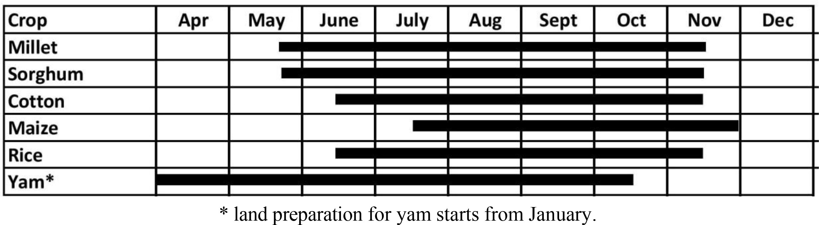
42]. The northeastern part of the catchment forms part of the Pendjari National Park in West Africa. The main source of employment for inhabitants of the catchment is agriculture. Major crops cultivated are cotton, maize, sorghum, millet, yam and rice. Sorghum and millet may be intercropped, while yam is sometimes intercropped with rice, maize, okra, agushie,
etc. Cotton is cultivated exclusively for export (the Government of Benin purchases the produce). The remaining crops are cultivated either for subsistence or for commercial purpose. Millet and sorghum are mostly for house consumption, while maize, rice and yam are normally sold in part to raise income for the household. Farm sizes are small. The authors of [
43] estimated that about 50% of farms in northwestern Benin are less than 1.25 ha in size. Due to the ease of marketing and the financial benefits associated with it, cotton fields dominate in this area and are normally bigger than that of other crops. It is estimated that about 50% of farm land in northwestern Benin is under cotton cultivation [
43]. Cotton farmers receive support from the government in the form of seeds, fertilizer and pesticides during the cropping season.
4. Methodological Approach
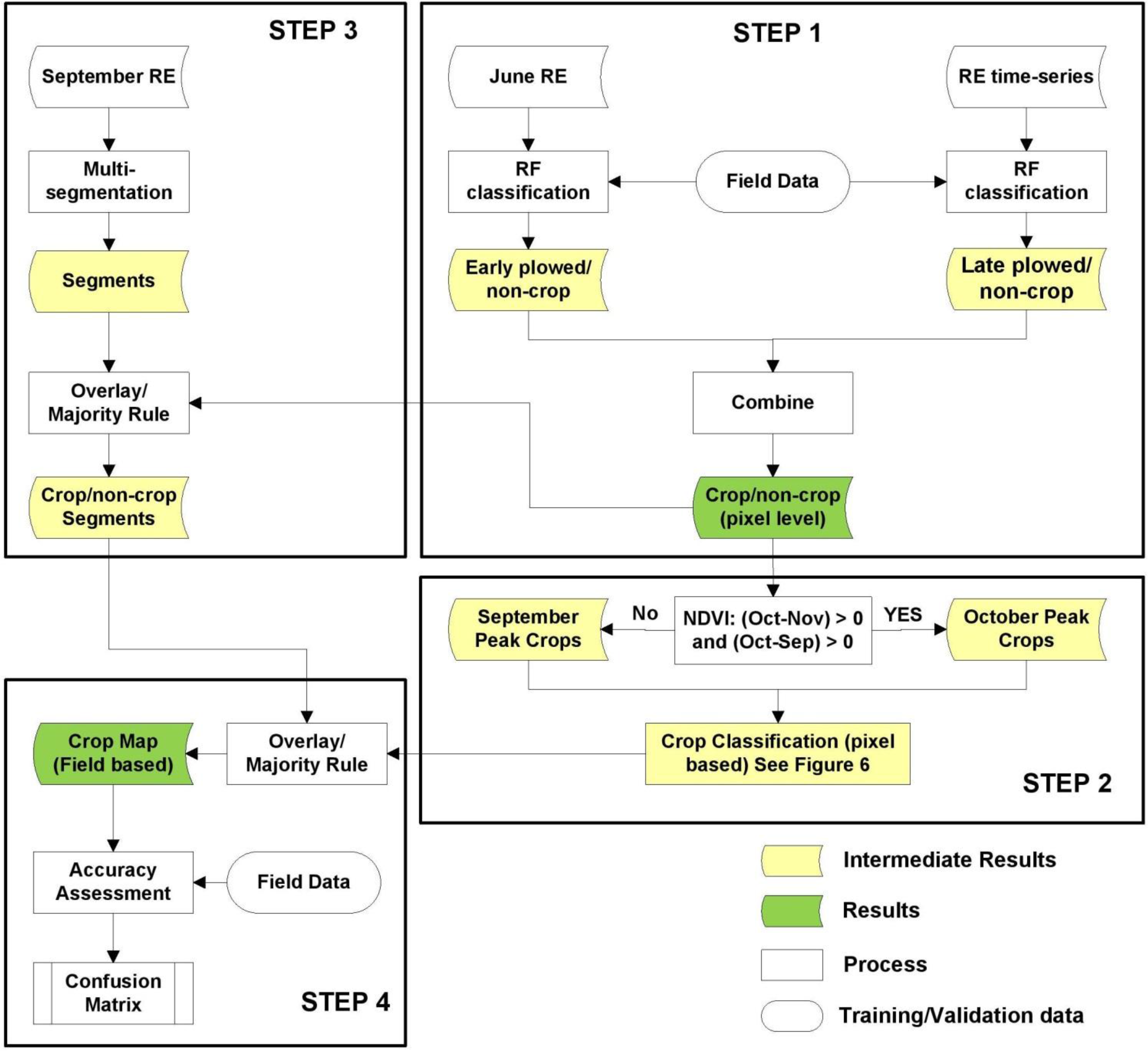
The methodological approach adopted in this study includes four main steps (
Figure 4). In Step 1, a crop mask (
i.
e., separation between cropped and non-cropped areas) was derived. This step was necessary to reduce confusion between crops and surrounding natural/semi-natural vegetation, due to high similarities between the phenological cycles of these two classes [
36,
58]. In the second step, a per-pixel crop classification was conducted on the derived crop mask (
i.e., cropped areas only) using a hierarchical classification scheme and the random forest classification algorithm. Crop classification using per-pixel approaches often results in a “speckled” output due to high spectral within-field heterogeneity [
8]. In West Africa, this situation is further aggravated by a heterogeneous landscape [
12]. Recent studies have overcome this challenge by overlaying per-pixel classification results on parcel/field boundaries and assigning the modal class within each field as its class [
5,
23]. This approach has been found to improve classification accuracies [
32,
37]. In line with this, the third step of the methodological approach involved the derivation of field boundaries in the study area using the RE images and a segmentation algorithm. These boundaries were combined with the results of Step 2 to produce a per-field crop map. In Step 4, the accuracy assessment was conducted on the per-field crop map using independently surveyed fields (
Table 2). The sections below detail each of the four steps.
4.1. Classification Algorithm
The random forest (RF) classification algorithm [
59], which belongs to the class of ensemble classifiers, was used for classification. The RF package in the statistics software “R” was used [
60,
61]. This algorithm automatically generates a large set of classification trees (forest), each tree based on a random selection of training samples and predictors. Predictors are the spectral bands of RE (
i.e., original + indices) and TSX (see Sections 3.1 and 3.2). Training samples are derived by overlaying training areas/polygons on the predictors and extracting the corresponding pixel values. By building several classification trees, RF overcomes the generalization errors associated with single classification trees and, thus, increases the classification accuracy [
62]. Each tree in the forest casts a unit vote for the most popular class. The classification output is determined by a majority vote of the trees. RF conducts an internal validation (out-of-bag error rate) based on training samples that are not used in the generation of the trees [
63]. This error rate served as an initial assessment of classification accuracy and as a guide to the selection of appropriate parameters for each run. For all classifications, a maximum of five hundred trees were generated, while the default number of predictors (
i.e., square root of total number of predictors) to be tried at each node [
60] was used. The RF variable importance measure [
60] was used to identify the most important predictors in all classifications. The mean decrease in the Gini coefficient served as a measure of variable importance.
4.2. Derivation of a Crop Mask
Derivation of a crop mask prior to crop classification has been found to improve classification accuracies [
64]. This is particularly important in heterogeneous landscapes, such as West Africa, where farming is done around hamlets and in bushes. The practice of integrated crop and livestock systems [
65] also results in grasslands that are close to fields, which are often left for animal grazing. Consequently, crop mapping on full-image scenes results in considerable confusion between crop/non-crop areas.
Ploughed fields or fields at early vegetative stages have unique spectral characteristics compared to surrounding natural/semi-natural vegetation, due to high reflectance from the background soil. Thus, an image acquired during the ploughing or early crop stages is important for accurately discriminating cropland from surrounding land uses and covers. Since ploughing in the study area begins in late April/early May, the RE image acquired on 13 June was first classified to identify fields that had been ploughed as of the time the image was acquired. Two classes (early ploughed/non-crop) were considered at this stage. The areas identified were masked out from the RE image time series. Due to variable planting dates in the study area and the fact that some crops are cultivated a bit later after the onset of the rainy season (e.g., maize), a considerable number of fields in the study area had not been ploughed at the time of the June acquisition. Therefore, a second classification was performed to identify these fields. This classification was performed using all six available RE images, with only two classes (late ploughed/non-crop) considered as previously. Cropped areas identified in both classifications (early and late ploughed) were combined to derive a crop mask. A per-pixel accuracy assessment was performed by comparing the final results (crop/non-crop) with reference data obtained from the field campaign. Overall accuracy, producer’s accuracy and user’s accuracy [
66] were computed.
4.3. Crop Classification
4.3.1. Experimental Design
The objective of this research was to investigate whether SAR data acquired during the cropping season can complement optical data to improve classification accuracies in the study area. In order to achieve this objective, four experiments were conducted with different image combinations (
Table 3). In Experiment (A), four RE images acquired in April, May, October and November were used for classification. This selection was made based on analysis of historical Landsat acquisitions (1984–2011) in the region. Historical acquisitions reveal a high possibility of obtaining optical imagery for these months. This is mainly due to the fact that these months fall largely outside the peak rainfall season, during which there is relatively lower cloud cover with better chances of obtaining cloud-free optical images. Thus, this experiment was conducted to determine the accuracies that can be obtained with such a time-series. Experiment (B) assessed the improvement in classification accuracy when SAR imagery acquired during the peak cropping season (May, June, July, August) was added to the RE time series in (A). Experiment (C) assessed the accuracy of classification when all available RE images were used for crop classification, while Experiment (D) considered the use of all available RE and TSX images.
4.3.2. Classification Approach
Crop classification was performed on the generated crop mask to discriminate five crop types/groups. These are cotton, maize, rice, yam and millet/sorghum. Millet and sorghum were combined into one class (cereals) due to similarities in their structure, planting dates and the fact that they are often intercropped [
67]. The initial classification of all the five classes using different image combinations resulted in high levels of confusion between the classes.
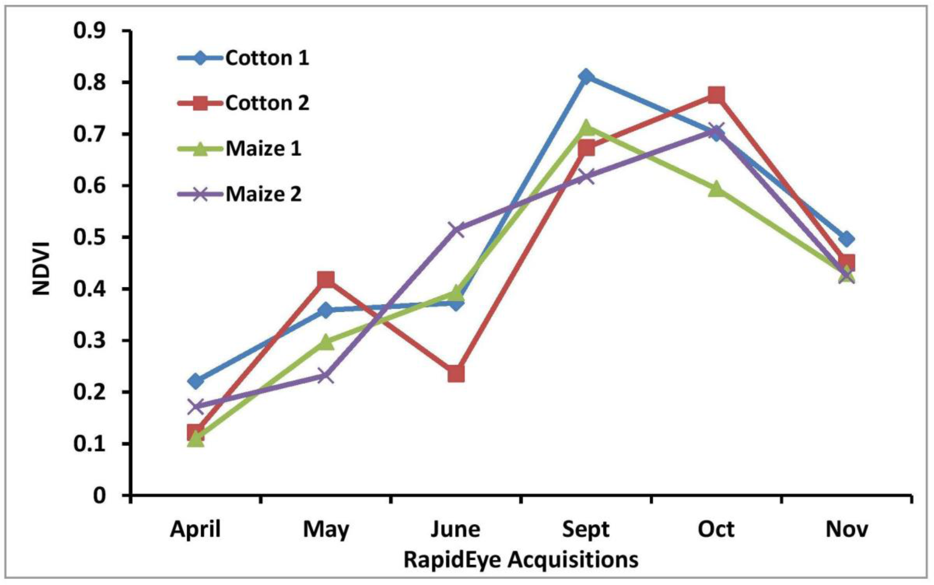
A study of the RE NDVI temporal profiles of the training data revealed that variable planting dates of the same crops, which leads to temporal within-class variability, was possibly the cause of the confusion. As depicted in
Figure 5, two cotton fields (Cotton 1 and 2) exhibit different temporal profiles, with one having a peak in September and the other in October. Maize 1 has a temporal profile similar to that of Cotton 1, with both having a peak in September. Farmers in the study region subjectively decide on when to plough and seed. Some farmers plant late in the season, due to poor rains, while others still follow the traditional cropping calendar regardless of the amount of rainfall received. This situation could lead to different crops (e.g., Cotton 1 and Maize 1) exhibiting similar phenological profiles, while the same crops (e.g., Cotton 1 and Cotton 2) would exhibit different phenological profiles. The authors of [
68] identified similar challenges (temporal within-class variability), especially for rice cultivation, in the Khorezm region in Uzbekistan, Central Asia. They noted that temporal segmentation of MODIS time series results in a better representation of crops that exhibit temporal variability in phenology. However, temporal aggregation of information was impossible for this study, due to the heterogeneity of the time series available here (SAR and optical data, irregular acquisitions).
In order to reduce the effect of this confusion, two separate masks, October and September peak, were created from the crop mask based on the NDVI images of the September, October and November RE images (
Figure 4). Mask 1 included all fields that have an NDVI peak in September, and Mask 2 included fields with an NDVI peak in October. The October and September peak masks constituted 65% and 35% of the crop mask, respectively, suggesting that the majority of the crops in the study area reach their peak (full development) in October. Separate classifications were performed on the two masks to reduce confusion due to variable planting dates. Fifty-four out of the eighty-four training samples (see Section 3.3) were used to classify the October peak mask, while thirty samples were used for the September peak mask.
Figure 6 details the classification approach adopted to classify the five crop types on each of the masks described above. A three-level hierarchical scheme was implemented to sequentially differentiate the different crop types. At each level, several band/image combinations were tested (depending on the experiment being conducted; Section 4.2.1) during classification to determine the optimal combination for discriminating the classes under consideration. At the first level, an RF classification was performed to separate two broad crop groups (rice/yam and cotton/maize/cereals). These two crop groups were determined based on the results of an initial one-time classification involving all crops, which revealed little confusion between the two groups. A mask was created for each group for subsequent analysis. At the second level, different RF classifications were performed to separate yam from rice and cotton from maize, millet and sorghum. A final classification was conducted at the third level to separate maize from millet/sorghum (cereals). Results obtained for individual crops at Levels 2 and 3 were combined into a final crop map (at the pixel level). A corresponding per-field crop map was produced by overlaying the per-pixel crop classification results with field boundaries derived through image segmentation (Section 4.3). The modal crop class within each field boundary was assigned to it.
4.4. Derivation of Field Boundaries
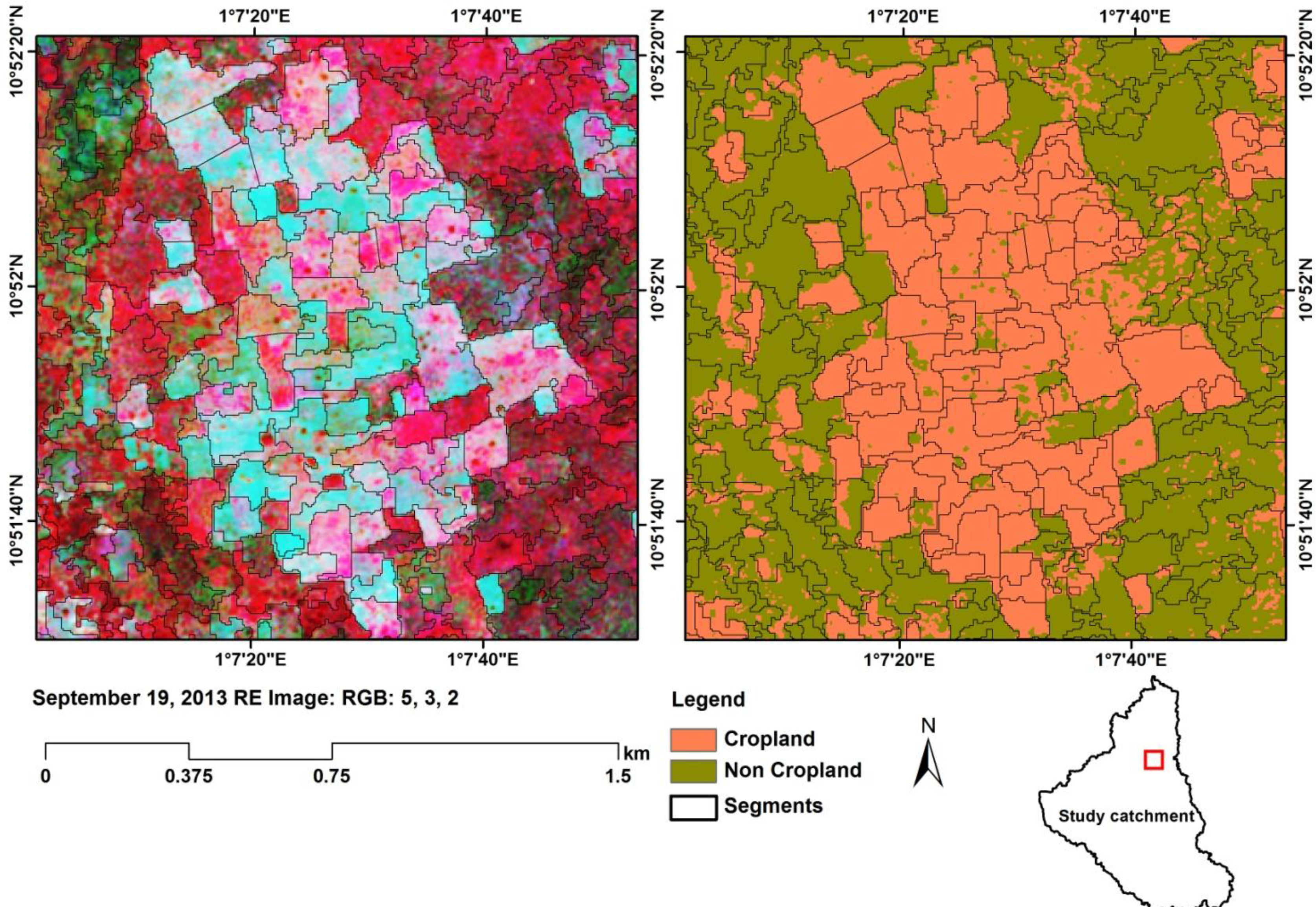
A cadastral map showing the field boundaries in the study area does not exist. Therefore, field boundaries were derived from the RE image acquired on 19 September. This image was chosen because it presented the best contrast between fields, which can be attributed to structural differences between the different crops at the time of acquisition. For example, maize fields, which are generally cultivated later in the season (late July/early August), will, by mid-September, be at the mid-vegetative stage, while millet/sorghum, which are planted much earlier in the season (May/June), would be at the seed development/senescence stage.
The eCognition Developer Software (8.7) [
69] was used to conduct a multi-resolution segmentation of the image. Due to a higher between-field contrast in the NIR and red edge bands, the weights of these bands were doubled. Different parameter sets of scale, shape and compactness were tested in segmenting the image. The result of each test was validated against twenty-four manually-digitized fields (from the September image) by comparing their corresponding areas and calculating the mean absolute error (MAE) and the mean error. The result of the parameter set with the best statistics was selected.
Separation between crop and non-crop segments was achieved by overlaying the segmentation results with the per-pixel crop mask derived in Step 1 (Section 4.1) and assigning the modal class in each segment to it [
5,
37,
38]. For the crop segments, the percentage of crop pixels in each segment was extracted. This was to provide a reliability measure for the derived crop segments.
4.5. Accuracy Assessment
Accuracy assessment was conducted on the per-field crop maps with a total of 76 fields evenly spread over the study area (
Figure 1). The overall accuracy, producer’s accuracy and user’s accuracy [
65] were determined. Additionally, the F1 score (
Equation (6)) [
70,
71], which combines producer’s and user’s accuracy into a composite measure, was computed for each class. This measure enables a better assessment of class-wise accuracies. The score has a theoretical range between “0” and “1”, where “0” represents the worst results, while “1” is the best.
5. Results and Discussion
5.1. Derivation of Crop Mask
Table 4 presents the confusion matrix for the per-pixel evaluation of the crop mask. The approach adopted (mapping plowed fields on the June RE image and the remaining fields on the available time series) reduced the confusion between crop and non-crop areas. An overall accuracy of 94% was achieved, while the producer’s and user’s accuracy were consistently above 90%.
5.2. Image Segmentation
The segmentation results of the different parameter sets (scale, shape, compactness) were tested against twenty-four manually digitized fields from the September RE image. The manually digitized fields ranged in size from 0.5 to 4 ha, which is representative of farm sizes in the study area, although most fields are under 2 ha [
43]. MAE was computed for each segmentation result based on the areas (ha) of the corresponding polygons (
i.e., manually-digitized and segmentation). The best parameter set was found to be 75, 0.5 and 0.5 for scale, shape and compactness, respectively.
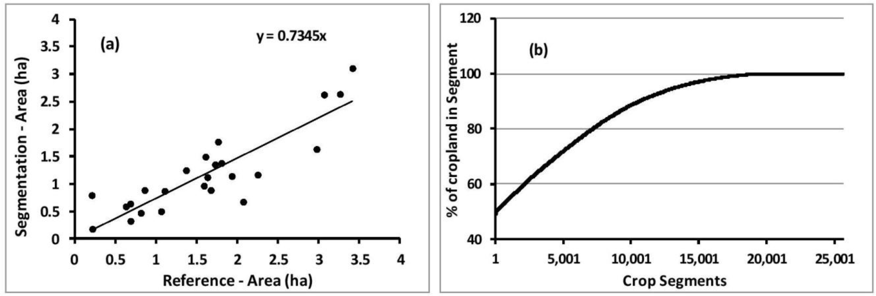
Figure 7a shows a plot of the manually-digitized fields against corresponding fields from the best segmentation. An MAE of 0.46 was obtained.
There were more cases of underestimation than overestimation. These errors can be attributed to many factors. First is the irregularity in field sizes and shapes in the study area. Fields vary in size depending on whether the cultivation is for subsistence or for commercial purpose. Cotton and maize fields, for instance, tend to be relatively larger than millet/sorghum, due to the commercial benefits farmers get from these crops. Additionally, some fields tend to be very irregular in shape, because of the use of manual approaches to land clearing. Intra-field color variation, which could be caused by spatial variation in soil fertility or differences in fertilizer application, was found to be one of the causes for the underestimation witnessed. This situation occasionally resulted in multiple segments within a field. The occurrence of natural/semi-natural vegetation (e.g., trees) on or at the boundaries of fields also resulted in under- or over-estimation of segments, since the field boundaries change depending on the position of the tree(s).
The results of the segmentation were divided into crop and non-crop segments by overlaying them with the per-pixel crop mask (Section 4.1) and assigning the majority class (from the crop mask) to the corresponding segment (
Figure 8). For each segment labeled as cropland, the percentage of cropland pixels in it was noted.
Figure 7b presents a plot of the crop segments and the percentage of cropland pixels in each (percentages were sorted in ascending order). Segments that had less than sixty percent cropland were found to be mainly farms around hamlets. These were mostly over-segmented and sometimes included the hamlets themselves. Cultivation around hamlets is common in West Africa. In this watershed, however, there are not many, hence the relatively few number of fields in this category. Thirty percent of all segments were found to be pure cropland (
i.e., 100% cropland pixels). These were found to be in areas of intensive cultivation, with little or no natural/semi-natural vegetation.
Segments with a crop percentage of between eighty and hundred percent were found to have varying numbers of trees in the polygon. Sub-canopy cultivation is common in West Africa, which often leads to a highly fragmented landscape. The trees serve as resting places for farmers when they are on the farms. The category of crop segments that had a cropland percentage of between sixty and eighty were found to be close to or in the midst of natural/semi-natural vegetation. Thus, the relatively low percentage of cropland pixels (60%–80%) noticed in these segments can be attributed to confusion between the two classes (crop and natural/semi-natural vegetation) or over-segmented crop fields that extended into the natural/semi-natural vegetation. For most of these fields, manual corrections were made.
5.3. Crop Classification
5.3.1. Accuracy Assessment
A per-field accuracy assessment was performed for each of the experiments outlined in Section 4.2.1.
Tables 5 and
8 present results for each experiments, while
Figure 9 is a plot of the class-wise accuracies (F1 score) for the different experiments.
Experiment (A), which was conducted with only RE images acquired in April, May, October and November, achieved an overall accuracy of 52%. There was considerable confusion between all classes, especially between rice and yam, which had an F1 score of 0.47 and 0.25, respectively. The relatively high confusion between the two classes can be explained by the intercropping of yam and rice, mostly on yam fields. Yam is cultivated in mounds (heaps of soil). This practice creates gullies between adjacent mounds, where farmers, in their bid to maximize the utilization of their land, cultivate rice. Some farmers also cultivate maize, okra and agushie on the same field. During flooding months, water collects in the gullies and provides the needed water for the rice. This practice is believed to be the main source of confusion between the two classes. Cereals (millet/sorghum) and maize had an F1 score of 0.5 and 0.52, respectively. Four cereal fields were misclassified as maize and vice versa. This can be attributed to the image time series analyzed in this experiment. The NDVI image of the May acquisition was used to separate these two classes. Since most maize fields were plowed in July/August, the NDVI of these fields were higher than plowed cereals fields in May, allowing for separation between the classes. However, not all cereal fields had been ploughed at the time of the May RE acquisition. This means some cereal fields behaved spectrally similar to that of maize, hence the confusion between the two classes. Cotton had the highest F1 score of 0.74 (owing to a high user’s accuracy of 81%). There was, however, some confusion between cotton and cereals, which can be attributed to similarities in their cropping calendar and the inability of the analyzed temporal sequence to achieve a complete separation between the two.
The overall accuracy achieved in Experiment (B) was 62%, an increment of 10% over that of (A) (
Table 6). This experiment considered the RE images used in (A) plus the available TSX time-series. With the exception of maize, all the classes improved in accuracy compared to the results of Experiment (A). Notable are rice and yam, which increased in their F1 score from 0.47 to 0.69 and 0.25 to 0.42, respectively. The F1 score of cotton also increased by about 10% from 0.74 to 0.81. The producer’s accuracy of maize reduced from 53% to 47%, while the user’s accuracy remained the same, resulting in a slight decrease in the F1 score from 0.52 to 0.48. This was due to an increase in confusion between maize and cotton compared to the results of Experiment (A).
In Experiment (C), the use of all available RE time-series (April, May, June, September, October and November) resulted in an overall accuracy of 60%. With respect to Experiments (A) and (B), the cereals class increased in the F1 score by 26% and 9%, respectively, while the corresponding increase in maize was 25% and 35%, respectively. These improvements in class accuracies are attributable to the inclusion of the June RE image in this experiment. As previously explained, the late cultivation of maize was the best way of separating it from the cereals class. Since most cereal fields had been ploughed as of the time of the June acquisition, and most maize fields not; a better separation of the two classes was possible using the June NDVI image. As in Experiment (A), rice and yam performed poorly in this experiment, with yam having an F1 score of 0.21. The F1 score of cotton increased slightly over that of Experiment (A), but decreased marginally compared to results of Experiment (B).
Table 8 shows the results obtained for Experiment (D). An overall accuracy of 75% was achieved. Here, all available RE and TSX time-series were considered in the classification. Class-wise accuracies (producer’s, user’s, F1 score) were better than all other experiments. An F1 score of at least 0.7 was achieved for all classes, except yam. Cotton, like in all previous experiments, had the best class accuracy (F1 score = 0.86), followed by cereals, rice and maize. These improvements can be attributed to the use of all the available RE and TSX time-series, which covers the full cropping season.
Figure 10 provides a detailed look of the per-pixel and per-field results obtained for this experiment.
A minor limitation of the hierarchical approach adopted, which could negatively affect reported accuracies, is error propagation [
5,
72]. First, the commission and omission errors incurred in generating the crop mask are inherent in the reported crop classification accuracies. Second, errors in classifying a crop class/group at any stage of the hierarchical crop classification scheme will be propagated into subsequent classifications. Thus, although the scheme was implemented to reduce confusion between classes, it may have resulted in some errors not being accounted for in the presented accuracies.
5.3.2. Contribution of TSX Data to Crop Mapping
Results obtained for Experiments (B) and (D) indicate that the inclusion of TSX data increased classification accuracies by 10% and 15%, respectively. Owing to the classification approach adopted, it was possible to identify the contribution of radar in improving classification accuracies. For each RF classification performed at the various levels of the hierarchical scheme, the variable importance measure, which indicates the relative importance of the variables/predictors used [
73], was extracted.
Table 9 shows the various levels of the classification scheme and the five most important predictors (out of all predictors) used to separate the classes at each level. The table indicates that the best separation between rice and yam was achieved by the multi-temporal TSX data. This fact is also evident in
Tables 6 and
8. The class accuracies (F1 scores) of yam and rice increased by at least 40% when TSX data were included in the classification ((B) and (D)) compared to the use of RE images only ((A) and (C)). This can be attributed to the sensitivity of radar systems to land surface characteristics, such as soil moisture and roughness [
74]. Due to the cultivation of yam in mounds (soil heaps), these fields have a rougher surface characteristic compared to rice-only fields. Thus, backscatter intensities are expected to be higher for yam fields than rice. Additionally, previous studies that used SAR data for crop mapping have distinguished between “broad leafed” and “fine/narrow leaf” crops and noted the usefulness of radar data in differentiating them based on their canopy architecture [
24,
25]. Broad-leaved crops have higher backscatter intensity than fine-leaved crops, due to a high absorption of the radar signal in the latter [
75]. In this regard, yam, which can be categorized as broad leaf, will have higher backscatter intensities than rice, which can be considered as fine leaf.
Figure 11a depicts a feature space plot of the July TSX VV and VH intensities for rice and yam. The figure shows higher intensity values for most yam fields compared to rice, although some confusion between the two classes still exists.
The TSX data also contributed to improving the separation between cotton and maize/cereals. For example, the class accuracies (F1 score) of cotton increased by at least 10% when TSX data were included in the classification (Experiments (B) and (D)) compared to the use of only RE data. Out of the multi-temporal TSX data, the August acquisition was found to be important for this separation. This could be due to differences in the canopy structure (e.g., leaf shape and size) of cotton, on the one hand, and maize/cereals, on the other.
Figure 11b shows a feature space plot of the August VV and VH intensities for cotton and maize/cereals. The plot shows higher intensities for most cotton fields compared to the other classes, although some confusion is still evident. The relatively shorter wavelength of TSX (compared to, e.g., C-band Radarsat and L-band ENVISAT) and its resultant high sensitivity to vegetation canopy contributed to the improved class separation when TSX was included in the classification. Previous studies that used TSX for the classification of agricultural areas highlighted its capability to observe small-scale vegetation changes due to its lower penetration depth [
19,
20,
25]. For example, in a multi-frequency SAR integration study to map major crops in two sites in Canada, [
34] found that multi-temporal TSX produced a better overall classification accuracy than multi-temporal C-band RadarSat-2.
In all classifications involving the TSX data, the VV polarization was found to better discriminate crop types than the other TSX bands used in the classification (VH, K0, K1). In the case of cotton and maize/cereals, for instance, the VV polarization is the only TSX band that came within the five most important variables (based on the RF variable importance measure) in discriminating the two classes. Previous studies [
8,
23,
34] also noted the superiority of the VV polarization in separating certain crop types (potatoes and cereals) over the VH polarization. The sensitivity of the VV polarization to different canopy structures was found to be the main reason for their ability to discriminate different crop types. This reason is applicable in this study, owing to the differences in canopy architecture between cotton and cereals/maize, as well as rice and yam.
5.4. Reliability of Modal Class Assignment
Previous studies that incorporated vector field boundaries and per-pixel results by assigning the modal class to each field polygon have noted the superiority of such approaches over only per-pixel classification results [
8,
37]. However, the reliability of the results obtained in the modal class assignment depends on the reliability of the per-pixel classification [
5]. In instances where the number of classes being considered are high, interclass confusion in the per-pixel result could lead to a particular field having a modal class with a small proportion (e.g., 25%). Thus, an idea of the proportional cover of the modal class within each field could provide information about the level of confusion within the field, as well as the reliability of the approach (
i.e., modal class assignment) adopted.
In this study, the proportion of the modal class in each correctly classified field was analyzed together with the local/within field variance (
i.e., a measure of the number of classes). The objective is to ascertain the reliability of the approach adopted (modal class assignment) and to gauge the interclass confusion in the per-pixel classification result within each field. This analysis was conducted for Experiments (A) (without radar) and (B) (with radar) due to similar patterns in Experiments (B) and (D).
Figure 12a,b presents a plot of the proportion of modal class against local variance per each correctly classified field for the two experiments. The number of correctly classified fields per crop type is indicated in parenthesis. The plots reveal that the proportion of modal class for most correctly classified polygons exceeded 50% in both experiments.
In Experiment (A), the cereal class had the lowest average proportion of modal class of 57% and the highest average within-field variance of 0.81. This suggest a high interclass confusion on cereal fields, which can be attributed to difficulty in separating cereals from maize and cotton with the time-series used. Maize, rice and yam had an average proportion of modal class of 70%, 74%, 88% and average local variance of 0.34, 0.32 and 0.3, respectively. This indicates that correctly classified fields in these classes were relatively homogeneous, and the assigned class was indeed the dominant class. Cotton fields had a similar average proportion of modal class of 74%, but a slightly higher average local variance of 0.51.
The average proportion of modal class for cereals improved to 62% in Experiment (B), while the average variance reduced to 0.58. This was mainly due to a better separation between cereals and cotton, owing to the inclusion of the TSX data. Likewise, the average proportion of modal class for cotton and maize improved to 78% and 72%, while average variance reduced to 0.43 and 0.25, respectively. The situation for rice and yam was, however, different. The average proportion of modal class for rice and yam reduced to 68% and 62%, while average variance increased to 0.42 and 0.91, respectively. This suggests a relatively higher interclass confusion on rice and yam fields. Although the inclusion of the radar data improved the separation between the two classes (by correctly classifying three and two additional rice and yam fields, respectively), the proportion of modal class on these additional fields were typically between 50% and 60% (
Figure 12b).
6. Conclusions
This research integrated multi-temporal RapidEye (RE) and multi-temporal dual polarimetric TerraSAR-X (TSX) data (VV/VH) to map crops in northwestern Benin, West Africa. The study demonstrated the ability to map crops and crop groups in a region where the poor availability of optical data, complex cropping systems and a highly fragmented landscape has hindered crop mapping efforts for years. A hierarchical classification scheme that adapts to the challenges highlighted above was implemented to map crops and crop groups using the random forest (RF) classification algorithm. Different image combinations were used to classify crops and crop groups at different levels of the hierarchical scheme. Four experiments were set up to ascertain the contribution of SAR data to improving classification accuracies in crop mapping in the study area.
Results indicate that the integration of RE and TSX data improved classification accuracy by 10%–15% over the use of RE only. The contribution of TSX data was mainly in separating rice and yam, as well as cotton and maize/millet/sorghum. The VV polarization was found to better discriminate crop types than VH polarization. The research has shown that if optical and SAR data are available for the whole cropping season, classification accuracies of up to 75% are achievable. This result is promising for West Africa, where accurate and up-to-date information on agricultural land use is urgently required to develop adaptation and mitigation strategies against the looming effects of climate change and variability. The methodology developed in this paper can be applied to other parts of the region to map crops and crop groups with comparable accuracies.
Varying planting and harvesting dates were found to be a major source of misclassification. In future studies, fields to be used for training and validation will be monitored continuously throughout the cropping season (from the ploughing stage to harvest) to gain a better understanding of the dynamics in the phenological cycles of same crops planted/harvested at different stages of the season. Continuous monitoring (year-to-year) of fields in this manner is necessary to understand the dynamics in cropping patterns and to inure to the benefits of future attempts at operationalizing agricultural land use mapping in the region.
The soon-to-be-launched Sentinel-1 satellite, which will provide free and open access SAR data in dual polarization mode (VV/VH) will greatly enhance crop mapping efforts in West Africa and other tropical regions worldwide. Day and night, all weather acquisitions will ensure the availability of data throughout the cropping season, which, when combined with freely-available optical data (e.g., Landsat 8), can deliver comparable or better classification accuracies than what has been achieved in this study.

 ,
, 


