Noise Reduction and Gap Filling of fAPAR Time Series Using an Adapted Local Regression Filter


Abstract
: Time series of remotely sensed data are an important source of information for understanding land cover dynamics. In particular, the fraction of absorbed photosynthetic active radiation (fAPAR) is a key variable in the assessment of vegetation primary production over time. However, the fAPAR series derived from polar orbit satellites are not continuous and consistent in space and time. Filtering methods are thus required to fill in gaps and produce high-quality time series. This study proposes an adapted (iteratively reweighted) local regression filter (LOESS) and performs a benchmarking intercomparison with four popular and generally applicable smoothing methods: Double Logistic (DLOG), smoothing spline (SSP), Interpolation for Data Reconstruction (IDR) and adaptive Savitzky-Golay (ASG). This paper evaluates the main advantages and drawbacks of the considered techniques. The results have shown that ASG and the adapted LOESS perform better in recovering fAPAR time series over multiple controlled noisy scenarios. Both methods can robustly reconstruct the fAPAR trajectories, reducing the noise up to 80% in the worst simulation scenario, which might be attributed to the quality control (QC) MODIS information incorporated into these filtering algorithms, their flexibility and adaptation to the upper envelope. The adapted LOESS is particularly resistant to outliers. This method clearly outperforms the other considered methods to deal with the high presence of gaps and noise in satellite data records. The low RMSE and biases obtained with the LOESS method (|rMBE| < 8%; rRMSE < 20%) reveals an optimal reconstruction even in most extreme situations with long seasonal gaps. An example of application of the LOESS method to fill in invalid values in real MODIS images presenting persistent cloud and snow coverage is also shown. The LOESS approach is recommended in most remote sensing applications, such as gap-filling, cloud-replacement, and observing temporal dynamics in situ where rapid seasonal changes are produced.
1. Introduction
The fraction of absorbed photosynthetic active radiation (fAPAR) is commonly used in ecosystem modeling because it has an important influence on exchanges of energy, water vapor and carbon dioxide between the surface of the earth and the atmosphere. The fAPAR has been also recognized as one of the fundamental essential climate variables (ECVs) by Global Terrestrial Observing System (GTOS) and Global Climate Observing System (GCOS) [1].
Space agencies and other institutional providers currently deliver various fAPAR products at different temporal and spatial resolutions over the globe taking advantage of available satellite data. A review is found in [1] and an intercomparison of products in [2,3]. However, vegetation attributes derived from polar orbit satellites, such as the EOS-MODIS, the VGT-SPOT or the Landsat-TM, often present considerable noise and poor coverage due to inefficient cloud filtering, high aerosol load, unaccounted surface directional effects, sensor problems or retrieval algorithm failures [4]. For example, MODIS fAPAR back-up retrievals have generally lower quality mostly due to residual clouds and poor atmospheric correction [5].
A well-recognized feature of fAPAR time series is a negative bias caused by snow coverage and unfavorable atmospheric conditions (cloud, ozone, dust, and other aerosols) that generally decrease near-infrared reflectance and increase reflectance in the visible, leading to spurious drops in the data [6–9]. Bidirectional Reflectance Distribution Function (BRDF) effects, mainly caused by anisotropic reflectance behavior of surfaces, may represent an additional source of uncertainty. BRDF effects can cause also positive errors in fAPAR.
Especially during winter, persistent clouds and snow coverage can originate large gaps in time series, which are not acceptable for many ecosystem or climate models [10,11]. These disturbances greatly affect the robust monitoring of land cover and terrestrial ecosystems and algorithms for time series filtering and reconstruction of fAPAR are thus required. Gap filling methods usually rely on temporal [12], spatial interpolation [13] or both [14]. Spatial interpolation has the advantage of minimizing local anomalies so that large-scale trends in regional to global vegetation phenologies can be better identified [15]. Nevertheless, spatial filters may fail when considering complex landscapes, with a high proportion of mixed pixels, where fAPAR could vary widely within a short distance [16]. This study has focused only on temporal methods.
Noise reduction and gap filling in time series is not straightforward. Filtering methods can be categorized as local or global in nature [17]. Local methods include: threshold (Interpolation for Data Reconstruction (IDR)), rank based (e.g., median, maximum or minimum filters) and linear/polynomial (e.g., moving average, adaptive Savitzky-Golay (ASG), locally weighted scatterplot smoothing (LOESS), Whittaker smoother, CACAO method, and smoothing spline (SSP) methods [18–24]). An advantage of the local methods is that they make no assumptions about the underlying nature of the processes responsible for the variability in the time series while taking advantage of the neighboring observation to generate an estimate. Nevertheless, for noisy and incomplete time series these methods are more limited and it becomes necessary to apply restrictions [25].
Global approaches consider model fits such as polynomial, Double Logistic (DLOG), asymmetric Gaussian (AG) [25–27], decomposition techniques based on Fourier analysis [28,29] or wavelet transforms [30,31]. Global methods are more suited to derive terrestrial biophysical parameters and extract seasonality information for phenological studies [25,32,33]. Nevertheless, these methods also suffer several drawbacks that limit their use. For example, the ASG filter outperformed global noise-reduction techniques when evaluated on the basis of RMSE [16]. Global methods assume an a priori phenological shape or magnitude that could make them not flexible enough to model the temporal response of irregular or asymmetric time series (e.g., high inter-annual variability) [19].
In the light of the abovementioned drawbacks, the present work is aimed to develop a robust methodology to provide temporally smoothed and spatially complete fAPAR time series. The study proposes an adapted LOESS to deal with the presence of noise and gaps in satellite data. The proposed LOESS method was enhanced based on an iterative reweighted algorithm to force the fAPAR curve to fit the upper envelope, thus removing contamination caused primarily by cloud and poor atmospheric correction. It is compared with four methods: DLOG, SSP, IDR and ASG, which have provided satisfying results. Hird and McDermid [34] showed that DLOG and AG techniques provide balanced performance to derive optimal times series metrics. Both methods are more flexible and effective than Fourier-based fitting method. The IDR technique compared favorably with DLOG and other smoothing techniques in [18]. The SSP method revealed a good performance in experiments involving different data sources [35]. The ASG performed better in most situations when it was compared with other seven filtering approaches such as DLOG, IDR among others [36]. Atkinson et al. [37] showed the higher performance of the Whittaker and Fourier approaches in most cases. This study also revealed that DLOG and AG did not perform well for areas with more than one growing season per year. The DLOG and ASG techniques were successfully applied to multi-temporal NDVI data sets over Africa and northern Europe, respectively, and both are easily implemented using TIMESAT software ( http://www.natgeo.lu.se/personal/Lars.Eklundh/TIMESAT/timesat.html) [25]. These methods have been used extensively on MODIS data in studies related to vegetation properties such as LAI [38] and vegetation indices [32]. The above analyses are limited and inconclusive, therefore there are still some aspects that need to be improved and completed.
This work shows the results of several experiments, which were conducted on simulated and real data sets in order to assess the performance of four methods to produce smoothed and gap-filled fAPAR data. Eight-day fAPAR time series were simulated with varying amounts of noise, and by adding gaps associated to persistent clouds and snow coverage. Typical profiles were extracted from MODIS time series that reflect the main seasonal behaviors and environmental disturbances. The applicability of the algorithm/methods on real MODIS imagery is also demonstrated.
2. Methods and Data
2.1. fAPAR Estimation
The 8-day fAPAR time series have been derived from MODIS data using the algorithm proposed by Roujean and Bréon [39]. The algorithm was previously adopted in Land-SAF (Satellite Application Facility on Land Surface Analysis) to deliver operationally fAPAR from SEVIRI sensor [4] ( http://landsaf.meteo.pt). Several works [40–43] have demonstrated the reliability of the proposed algorithm for retrieving daily fAPAR from medium and low-resolution satellite observations.
According to this algorithm [39], the fAPAR is obtained from the Renormalized Difference Vegetation Index (RDVI) as:
The reflectance in near infrared and red channels (NIR and RED, respectively) is computed in an optimal angular geometry in the solar principal plane (θs = 60°, θv = 45°, φ = 0°) from the BRDF parameters (k0, k1, k2).
The MODIS BRDF product (MCD43A1) used to estimate fAPAR is produced every eight days by using all high quality observations acquired by both Terra and Aqua over a 16 day period [43]. MODIS data from January 2001 to December 2012 were downloaded from https://lpdaac.usgs.gov/. The product is released in a global 500 m SIN Grid. The corresponding data quality product (MC43A2) is also used in this study: layer BRDF_Albedo_Band_Quality is used to identify the best quality data for the RED and NIR bands; layer Snow_BRDF_Albedo is used to choose snow free pixels; the land/water mask comes from the layer BRDF_Albedo_Ancillary.
To make the best use of the MODIS QC information, a simplified measure of the fAPAR quality was obtained for each pixel and date. For each individual band, the QC values corresponding to the combinations of the four first bits were considered (QC = 0 for the best quality; QC = 1 for good quality; QC = 2 for low quality when more than 7 observations are used in the model inversion; QC = 3 for the worst quality when between 3 and 7 observations are considered). Quality measurements were first computed for all the six input channels (i.e., three BRDF parameter (k0, k1, k2) in two MODIS bands (RED, NIR)) and then aggregated into a single quality control (QC) considering only the QC information of the bands used to compute fAPAR. Finally this ancillary information ranges from 0 (highest quality) to 6 (lowest quality).
2.2. The Proposed LOESS Method
The proposed adaptation of the LOESS method has been designed for reducing noise and suppress disturbances while maintaining the relevant data integrity. A flowchart with the adapted LOESS filtering approach is shown in Figure 1. LOESS is a locally weighted scatter plot smoother [21]. For each data value, yi, with associate time ti, i = 1, 2,⋯, N, a weighted linear least squares regression is performed to fit a d-th degree polynomial f(t) = c0 + c1t + c2t2 + ⋯ +cdtd to all 2n + 1 points in the moving window. Each smoothed is determined from the value of the polynomial at position ti in a window of size 2n+1 (being n the half-width of the filtering window size).
Similarly to previous studies [25,38], we have considered the characteristics of the satellite QC information to derive an improved fAPAR filtering. Observations from optimal MODIS reflectance (QC = 0) are initially assigned with a maximum quality score (wi = 1), invalid observations are discarded (wi = 0), and observations with a relatively low quality are assigned with a small weight, according to the following expression:
In addition to the QC information, a robust regression weight was defined:
In the above equation, Δyj is the difference between the first fitting data ( ) and the original fAPAR data (yj); σ is the standard deviation of Δyj and S is a free parameter (0.1 in this work) to be adjusted in order to correctly capture the upper envelope. To account for the negatively biased noise, the fitting is done in two steps.
The first step computes the weights only considering information provided by Equations (3) and (4). This allows considering QC information and increasing importance to the closest temporal steps to the smoothed point respectively. As aforementioned, the upper envelope of the fAPAR is more representative of the noise free data. To better capture it, in a second iteration of the process, the weights of each point are changed according to its residual (Δyj = yj − ). Thus, points of the original fAPAR data lower that the smoothed ones are assumed to be far from the upper envelop and assigned with lower weight according to Equation (5).
2.3. Methods under Comparison
In the DLOG method [25,27], a double logistic (asymmetric) function is fitted to data in intervals around maxima and minima in the time-series. The local model function has two linear parameters determining the base level and the amplitude and four non-linear parameters, which determine the shape of the basis function. DLOG implementation in TIMESAT uses a Levenberg-Marquardt algorithm [44] to solve non-linear least squares minimization problem.
The SSP method does a piecewise smooth (cubic polynomial) curve fitting for a time series in such a way that the first and second derivatives of the resulting curve are continuous. This method is adjustable through a single smoothing parameter λ, which controls the smoothness of the cubic spline. In the limit λ = 0, no departures of the data points from the fitted curve are found, whereas for high values of λ, it controls the trade-off between fidelity to the data and roughness of the function estimate. SSP is similar to the widely used Whittaker smoother [22] but without any adaptation to deal with the negatively biased noise in the time series.
The IDR filter [18] creates an alternative time series by computing the mean of the immediate preceding and following observations. The filtered value replaces the original value when the difference is above a certain threshold.
The ASG [19] filter is a generalized moving average, which preserves better the features of the underlying data value and its derivatives. The method is fast since coefficients are computed in advance [45] using an unweighted linear polynomial of a given degree, d. A quadratic polynomial (d = 2) is usually assumed (e.g., TIMESAT [25]). The main disadvantage of the method is that it requires a series of equally spaced data points.
2.4. Experiment Settings
In this work, the gaps in the time series with DLOG, SSP, IDR, and ASG were filled with a linear interpolation method. In case of the LOESS method, an adaption of the weights assignment to deal with missing data has been also considered. Thus, when no data was available a zero weight is assigned to that point and it is automatically interpolated.
To obtain the optimum parameters for each of the other four approaches, different fitting criteria were set to reconstruct the fAPAR time series over the nine reference sites in the study area. The selected methods were applied as close as possible to their standard implementation including the original parameterization as proposed by their authors. The SSP parameter was evaluated using the IMSL (International Mathematics and Statistics Library) routine CSSMOOTH, as implemented in the IDL (Interactive Data Language) environment using a Cross Validation procedure [46]. A similar implementation was evaluated in [35]. Although the optimum smoothing parameter λ for the spline curve was derived automatically, the goodness of the fit was confirmed by visual inspection. IDR was threshold to 0.02, as proposed by the authors [18] and used in recent studies [36]. Only a marginal improvement was found by a fine tuning of this parameter.
The ASG and DLOG approaches were adjusted interactively for each site in TIMESAT software to arrive at close fitting results. This manual adjustment has been recommended by the TIMESAT authors [47] and adopted in previous works [16,19].The six parameters of the DLOG model were obtained automatically by TIMESAT using the Levenberg-Marquardt method [44]. Initial values of the non-linear parameters are obtained by looping through a number of pre-defined model functions in a highly efficient search routine.
Both LOESS and ASG require specifying two parameters, the half-width of the filtering window size, n, and the degree of polynomial, d. The value of d determines the degree of filtering, but it also affects the ability to follow rapid changes [48]. In general, high d values may overfit to the data and give less smooth results [19]. For LOESS, if there are enough high quality data in the temporal window, a five-order polynomial (d = 5) was chosen for the weighted fit. Under extreme conditions, high percentage of occurrence of missing data (bad conditioned problem), LOESS adjusts a simpler curve (linear) to the sparsely available high-quality observations of the gap. Furthermore, to avoid to deal with such extreme conditions, we adopted a wide value of the half-width temporal window, i.e., n = 8. For ASG, the values d = 2 and n = 5. Chen et al. [17] recommended as appropriate parameters n in the range 4–7 and d in the range 2–4 (d = 2 is fixed by TIMESAT).
Using these optimal parameters, the five approaches were applied on different simulated and actual fAPAR time series. To assess the influence of the analyst subjectivity in the “tuning” step of each method, the same adjustment was achieved by three different analysts. Small differences were obtained for the considered statistical indicators.
2.5. Simulation of fAPAR Time Series
Typical fAPAR profiles were obtained based on 12 years (2001–2012) of actual fAPAR time series for a selection of representative sites [23,34]. Many different test scenarios were analyzed considering different levels of noise and missing data. The main steps of this procedure are:
- (1)
Selection of representative sites: Nine different homogeneous sites have been selected covering very different vegetation types in the study area (see Table 1). They were identified from a hybrid land-cover map by the synergistic combination of four classifications: CORINE, GLC2000, MODIS and GlobCover [49]. To ensure a good homogeneity and reduce the impact of misregistration errors, we imposed the agreement between the pixel label and modal land-cover label within a 3 × 3 pixel window (with a frequency of modal value higher than 6). We additionally imposed neighborhood pixel homogeneity of fAPAR time profiles (i.e., selecting maximum allowable variance values). For each site, 12-year periodic time profiles were obtained in a two-step process. First, a typical yearly noise free fAPAR profile was calculated for each site by averaging the pixel fAPAR values with the highest quality (QC = 0). Second, these annual profiles were replicated for 12 times in order to obtain statistically significant results.
- (2)
Addition of noise component and missing/invalid data. The underlying time series was subsequently perturbed by adding noise with varying levels. Noise components were generated using a random normal distribution N(μ,σ). The values for μ and σ were estimated using the range of noise found in the study area corresponding to different levels of quality in the data (high, medium, poor). In all cases, negative μ values were used, reflecting the perturbation in fAPAR time series due to cloud and poor atmospheric conditions. The noise was added to a uniformly random sample of points, whereas the rest of data was noise-free. To evaluate the impact of invalid values (gaps) in the reconstruction, two different types of gaps distributions were evaluated: (i) a random uniform distribution and (ii) a distribution of missing data extracted from real QC information of MODIS BRDF time series for selected sites. The simulation of typically adverse environmental conditions (e.g., persistent snow/cloud during winter time), which may lead to 2–4 months with consecutive missing data, is very interesting for our purposes.
2.6. Reconstruction Accuracy
The performance of the five filtering methods was quantified in terms of the mean absolute error (MAE) and root mean-squared-error (RMSE) as a measure of the accuracy, and the mean error (MBE) as a measure of the bias:
3. Results
3.1. Scenario 1: Different Levels of Noise in 25% of the Data
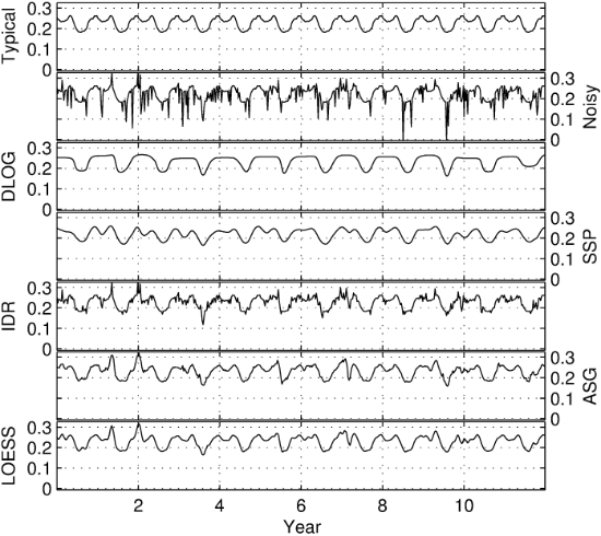
The first simulation scenario consisted of adding a noise distribution to 25% (random uniform) of the data points. 25 artificial datasets were thus generated with noise mean μ ranging from −0.01 to −0.05 (step = −0.01) and noise standard deviation σ ranging from 0.01 to 0.05 (step = 0.01). Figure 2 shows an example of fAPAR reconstruction under very noisy conditions corresponding to mosaic croplands, composed of small patches with different crop types. Four of the methods (except for the SSP) are designed for adaptation to the upper envelope. At giving priority to high values, this might cause biases toward relatively high values and overlook some useful information contained in low values. In particular, the high frequency of positive peaks remains in the case of the IDR method, at preserving the maximum value within its short temporal window. This method, although partially filters out the introduced noise, still produces shaky profiles with misleading peaks. The SSP, LOESS and ASG methods show to be effective in removing the high frequency noise while reproducing accurately the expected seasonal cycle. The cubic splines produce a remarkable smooth curve although its main drawbacks is that it does not preserve well some temporal metrics such as the amplitude of the annual fAPAR cycle and the rate of increase/decrease during the development and senescence periods.
Tables 2 and 3 present the average values of the performance measures over all the selected sites and methods. The LOESS and ASG are clearly more accurate (MAE, RMSE) and unbiased (MBE) than the rest of methods. In relative terms, both methods are effective in reducing both bias (|rMBE| << 100) and inaccuracy (rRMSE<<100).Where no distinct negative bias is present ASG filter performs better than others independently of the noise variance, while LOESS would be more properly applied in situ of negatively biased noise (a more realistic case). Conversely, the DLOG rather than enhancing the quality of the time series increases both types of errors when lowest bias and error magnitude are considered. The SSP method preserves the original bias (i.e., |rMBE| = 100) in all cases as expected since it is not adapted to correct negative biases due to clouds and poor atmospheric correction. Finally, the effectiveness of IDR to reconstruct the original timeseries is small, e.g., a marginal improvement in accuracy is found for simulations with μ = −0.01, σ = 0.01. It is important to note that the IDR shows an improved performance for the worst noise scenario considered in this study (μ = −0.05, σ = 0.05).
The influence of the noise parameters reveals that ASG and LOESS clearly outperform the other methods (see example in Figure 3). ASG performs slightly better than LOESS although LOESS exhibits also very high accuracies, with RMSE typically lower than 0.005. Overall, the reconstruction based on the DLOG algorithm generates the highest RMSE values because the method fails to capture components presenting multiple vegetation cycles per year (e.g., presence of a double phenology) in the original signals. The accuracy of this method becomes rather insensitive to the noise parameters. The performance of IDR and SSP approaches is also poor. The bias is the factor that most influences the accuracy of SSP, whereas the IDR is mainly influenced by the standard deviation σ. In general, the accuracy of IDR, ASG and LOESS increases considerably when noise mean values are far from zero since these methods rely on the assumption that the atmospheric contamination tends to drop fAPAR values, and therefore, higher fAPAR values are more acceptable than lower ones.
3.2. Scenario 2: Variation in the Proportion of Noisy Data
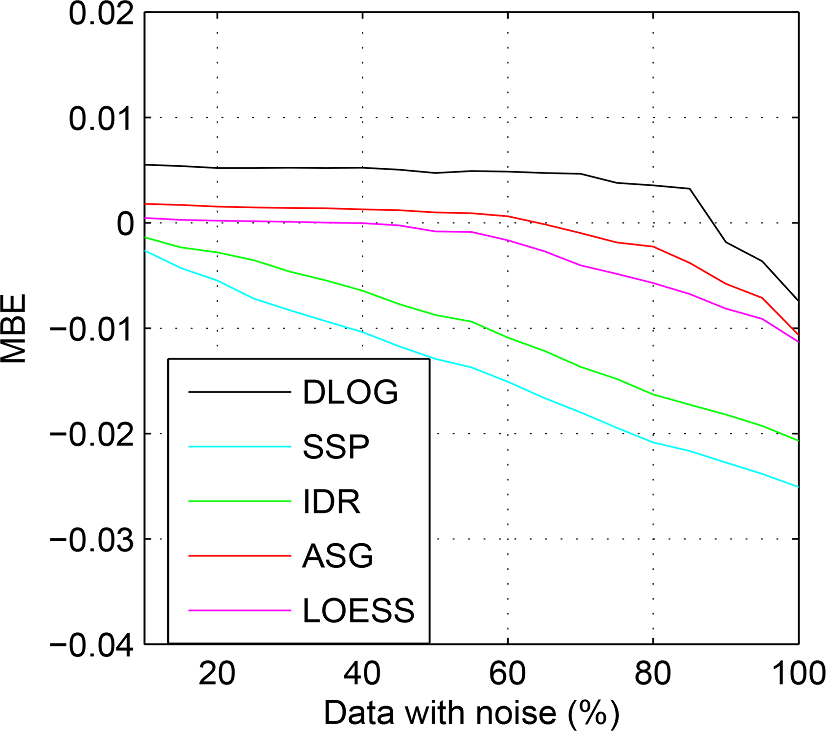
The second simulation scenario consisted of fixing the parameters describing the noise distribution (μ = −0.025, σ = 0.025) and varying the percentage of randomly distributed samples contaminated by noise. Figure 4 shows that the DLOG method produces fAPAR with a significant positive bias (MBE ∼ 0.004). Conversely, SSP and to a lesser extent IDR produce a high negative bias. This underestimation of fAPAR increases to inacceptable levels (MBE < −0.010) in proportion to the amount of data affected by noise and is related to the inability of these methods to capture the fAPAR envelope.
The LOESS presents generally a negligible bias (|MBE| < 0.002), but it increases leading to significant negative bias when the percentage of noisy data exceeds the 70%. When this scenario occurs, there is not an optimal method to reconstruct the upper envelope. This is partly due to the fact that the highest values are also generally affected by noise and therefore they have lower weights because of their associated QC values. The ASG method performs almost equally well and is even more robust when the time series is fully contaminated with noise especially when low biased noise is considered.
Figure 5 shows that the SSP and IDR clearly manifest a negative trend in their accuracy as the data affected by noise increases. The performance of the DLOG becomes acceptable when the percentage of contaminated data is high (>40%). However, as this situation is uncommon in the study area it difficult the practical applicability of the DLOG method.
The performance of the other methods, ASG and LOESS, is considerably better under situations of 20%–40% of contaminated data. Notably, the LOESS method reduces the noise disturbance to less than 1/4 of the original value. Again an increase of the LOESS and ASG error is observed for high percentage of noisy data (>50%). As aforementioned, this is related with the confounding factor of having highly positive noisy values. This scenario is unrealistic (noise usually cause rapid drops in fAPAR time series) and so it has not been considered in the adaptation of the proposed LOESS approach and in ASG.
3.3. Scenario 3: Randomly Distributed Missing Data
To assess the effectiveness of the four methods in presence of invalid values (gaps), we simulated noisy data with random uniform gaps in a two-step process. It is important to note that while LOESS deals with missing data in this parameterization, the other methods require gaps to be filled before its use. Following previous studies [16,19], a linear interpolator was used in these cases, independently of the size of the gaps. First, a set of noisy data was obtained by adding Gaussian noise (μ = −0.025 and σ = 0.025) randomly to 25% of fAPAR values. Second, different data sets were generated by assuming that a subset of the data presented invalid values. The proportion of gaps ranged from 5% to 30%.
Figure 6 shows the reconstructed fAPAR series for a mixed forest from a highly noisy time series. Compared with scenarios 1 and 2 (see Figure 2) all five methods produce smoother fAPAR profiles in presence of missing data. This is partly due to the use a linear interpolator to replace missing data, thereby limiting the temporal variance and performing an additional filtering. This may destroy relevant information (especially during long periods with missing data), as it is particularly evident in the case of the DLOG method that removes the peak of the second season (spring).
The reconstruction accuracy, in terms of MAE, is shown in Table 4. It is important to note that the methods are sorted according to their performance: LOESS provides the more accurate reconstruction (MAE in the range 0.0016–0.0025), followed by ASG (0.0025–0.0035), IDR (0.0044–0.0063), SSP (0.0072–0.0076) and DLOG, which provides the poorest results (0.0086–0.0088). The influence of the amount of gaps allows differentiating two different behaviors: (1) The reconstruction error of IDR, ASG and LOESS methods increases with the proportion of gaps in the series. (2) The error of DLOG and SSP seems to remain almost constant, partly because the increase in the number of gaps produces also a diminution in the number of noisy observations. In fact, both random temporal distributions are different and can be coincident, replacing noisy data with gaps.
3.4. Scenario 4: Influence of Missing Data Extracted from a Real Distribution
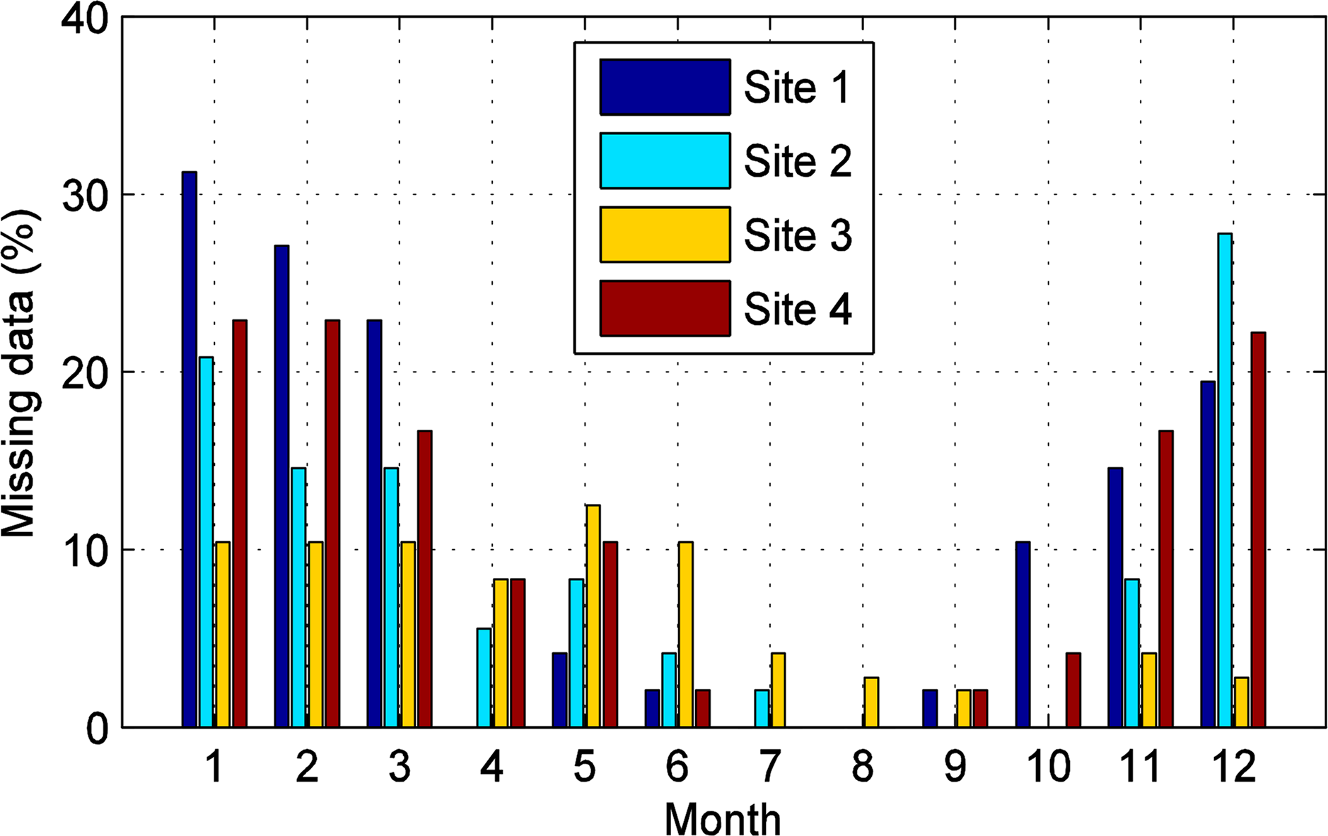
Data were simulated following the same procedure as in 3.3 but using a more realistic distribution non stationary (seasonal) of the missing data, since they were extracted from QC of MODIS BRDF time series. Four distributions of gaps were selected from four different sites, as shown in Figure 7. They characterize typical situations with missing values during long, continuous periods. In particular, the winter period (December–March) shows the highest frequency of invalid observations, which can be attributed to the periodical snow cover and high cloudiness in these regions. These simulations provide a more challenging scenario for testing the reconstruction ability of the five methods.
From Table 5, one can observe that DLOG and SSP are the most inaccurate methods. This is particularly exacerbating for the case of the DLOG, which provides relative values of improvement exceeding 100 (i.e., filtered fAPAR values depart from the “true” time series more than unfiltered ones). The worst results (highest MBE, MAE and RMSE) are found for DLOG method, although the performance of this method does not deteriorate at increasing the percentage of gaps (constant values of MAE). The SSP provides also biased fAPAR estimates since it was not designed to capture the upper envelope. The ASG turns out to be more accurate than the IDR method, providing a good fit to the original data (e.g., it reduces RMSE to less than 40%). As in previous results, the LOESS method provides the lowest biases and interpolates more precisely than the other considered methods, which can be partly due to the use of an optimal (non-linear) local interpolator. For example, the LOESS reduces more than 92% of the introduced bias (i.e., |rMBE| < 8%) and moreover it produces the higher accuracy (i.e., rRMSE ≈ 20%).
3.5. Application to Real Imagery
In this section, an application of the optimized LOESS algorithm in actual MCD43A1 (BRDF MODIS parameters) and MCD43A2 (BRDF QC) data has been considered to perform a qualitative analysis of the proposed methodology. Figure 8 shows the reconstructed and original fAPAR profiles corresponding to four sites with different vegetation types (needleleaf and broadleaf forests, shrublands and non-irrigated crops). LOESS performs as well as expected. That is, it is able to correctly capture the upper envelope, removing the unrealistic high frequency noise and reconstructing the present gaps in the time series for all the test sites considered. In addition, no significant differences are noticeable in comparison with Figures 2 and 6 when the synthetic noise was added to time series.
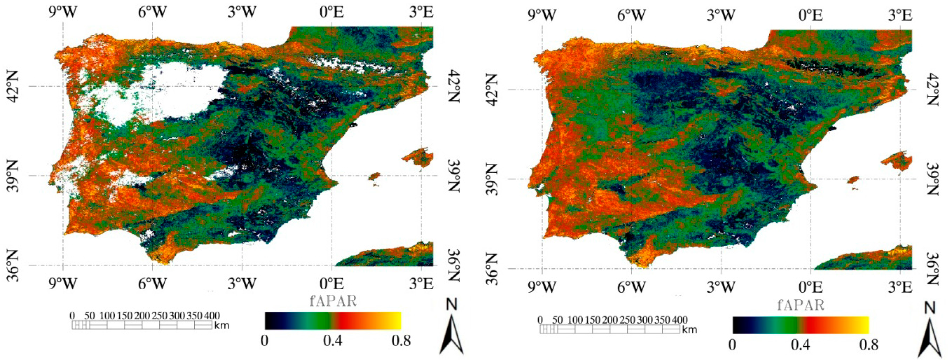
Finally, an example of the LOESS application to MODIS scale is shown in Figure 9 for the 1 January 2011 over the Iberian Peninsula. The visual comparison of the images indicates that the LOESS approach allows preserving almost identical the present spatial patterns after its application. In relation to the missing data, it is able to recover the information from neighboring dates without any visual noticeable spatial artifacts.
4. Discussion
In time series analysis of fAPAR products, inaccuracies in modeling the BRDF effects do not necessarily introduce a negative bias, but they can cause also positive errors in fAPAR. In this paper, the fAPAR was estimated using an optimal angular geometry. The use of a BRDF MODIS product (MCD43A1) may lower these influences, which could be more significant when using daily MODIS reflectance products due to the different image acquisition angles. For this reason, the common assumption that nearly always disturbances in these time series are caused by cloud cover and atmospheric contamination is accepted.
One typical problem in estimating the quality of the temporal reconstruction techniques is the unavailability of an objective reference data used to validate the results. In order to solve this problem, different approximates need to be made in practice. For example, [36] evaluate the performance of each filtering technique using as a reference the mean time series (assumed to be accurate) obtained from eight noise-reduction techniques, which is a simplification. Atzberger and Eilers [22] propose a range of approaches to test the plausibility of filtering results including class discrimination, pseudo-invariant targets, geostatistical noise estimation, etc. We have considered as the reference synthetic data representing multiple controlled scenarios. They include Gaussian noise distributions with varying amplitude and negative bias as well as occurrence of missing data extracted from real MODIS time series. Although, this Gaussian noise is commonly used in the literature to generate artificial time series [35,37,50], a red noise was further applied providing similar results. Future work is required to implement more realistic noise patterns since cloudy periods are usually concentrated in known period of the year.
The five considered approaches are computationally inexpensive and easy to implement, which make them applicable to generate fAPAR time series for regional and global studies. The methods are also applicable to NDVI and other remote sensing biophysical products such as LAI. Although finding one single optimal value for the two LOESS parameters that can be used in any circumstance is not feasible, we recommend a value around n = 8 for the half-width of the filtering window size and d = 5 for the degree of polynomial. Low differences were observed in the filtered curves under small perturbations of these parameters. The settings of the other four algorithms followed the original parameterization, showing to be relative robust against the analyst subjectivity.
The LOESS and ASG are clearly more accurate and unbiased than the rest of methods, since they are more flexible and best suited to capture the rapid seasonal changes in vegetation. An important cause for the moderate to poor performance of the SSP is that it assigns weights that are symmetric for points above and below the curve. In contrast, the other four approaches assume that clouds and poor atmospheric conditions usually depress fAPAR values. Hence they use some iterative tuning to remove these sudden events at punishing negative deviations in the weighted fitting, while preserving those compatible with the gradual process of vegetation change. One possible limitation is that this might cause biases toward relatively high values and overlook some useful information contained in low values.
Three of the approaches under comparison (LOESS, ASG and DLOG) incorporate ancillary data in the form of prior knowledge about the quality of the inputs (i.e., MODIS QC), which is routinely provided by most remote sensing products nowadays. In general, by maximizing the use of high-quality data to replace missing or poor-quality observations in the iterative process may enhance the quality of the filtering process. Further improvement could be obtained by modifying the original IDR and SSP algorithms in order to incorporate this MODIS QC.
The capacity of the methods resilient to periods of missing data to provide realistic interpolation is challenged in cases corresponding to medium to high fraction of missing data [16]. Techniques based on the processing of the time series as a whole (DLOG) were not demonstrated to perform systematically better than techniques based on a limited temporal window (LOESS, ASG, IDR) although they were expected to fill long gaps with the data available for the several years available in the time series. This is consistent with the finding that MAE values remain almost constant for DLOG in Tables 4 and 5, showing no influence of the amount of gaps. IDR was generally more faithful but showed poor capacity to fill long gaps, e.g., to reconstruct data contaminated by clouds during more than 4–5 consecutive observations. The ASG clearly outperforms the DLOG, the IDR and the SSP methods. These findings are consistent with other literature [36,50], showing better reconstruction regarding to other common techniques. Although the ASG is effective to denoise regularly sampled observations, its effectiveness diminishes in presence of missing records, particularly for long seasonal gaps (winter snow coverage and persistent cloud occurrence). Finally, the low RMSE and biases obtained with the LOESS method (rMBE < 8%; rRMSE < 20%) reveals an optimal reconstruction even in most extreme situations with long seasonal gaps. The linear approach could be excessive under prolonged periods of missing data. The LOESS method, which relies in a more complex fitting function (based on a wider temporal window with a higher degree polynomial to address rapid changes and an optimal weighting of observations), has allowed preserving and recovering the relevant information of the fAPAR.
5. Conclusions
Satellite land products generally need to be processed to remove data gaps and low quality data caused by cloud/snow contamination or algorithm limitations before they can be used in models directly. This work has developed an iteratively reweighted LOESS approach for noise reduction and gap filling of fAPAR time series. It was enhanced based on an iterative reweighted algorithm to force the fAPAR curve to fit the upper envelope, thus removing contamination caused primarily by cloud contamination and poor atmospheric conditions. The method provides a simple parameterization that converges to the upper envelope using only two iterations.
This approach has been compared quantitatively with four approaches, the DLOG, SSP, IDR and ASG methods, widely applied to reconstruct time series of remote sensing data. Results evidence the outperformance of the LOESS and ASG methods when compared with DLOG, SSP, and IDR over multiple controlled noisy scenarios. The DLOG, IDR and SSP methods introduce significant biases. The SSP, LOESS and ASG methods show to be effective in removing the high frequency noise while reproducing accurately the expected seasonal cycle, although the SSP is not robust against cloud contamination effects and hence it is unable to recover the fAPAR trajectories with different biases of noise. The LOESS and ASG are clearly more accurate and unbiased than the rest of methods, since they are more flexible and best suited to capture the rapid seasonal changes in vegetation. The other considered methods evidence also important drawbacks. For example, the DLOG has obtained the worst performance especially when the temporal evolution of the fAPAR presents more complex patterns.
Furthermore, LOESS is clearly the most accurate gap filler (MAE < 0.0022), even in situ with a large fraction of non-stationary (seasonal) gaps. The LOESS method does a credible job of filling long seasonal gaps due to its nonlinear nature and the use of wider moving window with a weighting scheme. This is partly due to its unique parameterization based on a nonlinear local interpolation in conjunction with a weighting scheme that optimally takes into account the ageing of the observations.
Although the selection of the optimal smoothing method depends greatly on the intended application, LOESS is expected to have the best performance in most applications, such as gap-filling, cloud-replacement, and observing temporal dynamics in situ where rapid seasonal changes are produced.
Acknowledgments
This research was supported by the projects: RESET CLIMATE (Spanish Ministry of Economy and Competitiveness, CGL2012-35831), ERMES (EU FP7-Space-2013, Contract 606983) and LSA SAF (EUMETSAT). Special thanks are due to the anonymous referees for their suggestions, which greatly improved the quality of the paper.
Author Contributions
All authors made significant contributions to the results, interpretation and presentation of this Article. All authors read and commented on the manuscript.
Conflicts of Interest
The authors declare no conflict of interest.
References and Notes
- Gobron, N.; Verstraete, M. ECV T10: Fraction of Absorbed Photosynthetically Active Radiation (fAPAR) Essential Climate Variables. Available online: http://www.fao.org/gtos/doc/ECVs/T10/T10.pdf (accessed on 26 August 2014).
- Meroni, M.; Atzberger, C.; Vancutsem, C.; Gobron, N.; Baret, F.; Lacaze, R.; Eerens, H.; Leo, O. Evaluation of agreement between space remote sensing SPOT-VEGETATION fAPAR time series. IEEE Trans. Geosci. Remote Sens 2013, 51, 1951–1962. [Google Scholar]
- Martínez, B.; Camacho, F.; Verger, A.; García-Haro, F.J.; Gilabert, M.A. Inter-comparison and quality assessment of MERIS, MODIS and SEVIRI fAPAR products over the Iberian Peninsula. Int. J. Appl. Earth Obs. Geoinf 2013, 21, 463–476. [Google Scholar]
- García-Haro, F.J.; Camacho, F.; Meliá, J. Vegetation Parameters Validation Report (VEGA VR), SAF/LAND/UV/VR VEGA/2.1; Available online: http://landsaf.meteo.pt (accessed on 19 June 2014).
- Yang, W.; Huang, D.; Tan, B.; Stroeve, J.C.; Shabanov, N.V.; Knyazikhin, Y.; Nemani, R.R.; Myneni, R.B. Analysis of leaf area index and fraction of PAR absorbed by vegetation products from the Terra MODIS sensor: 2000–2005. IEEE Trans. Geosci. Remote Sens 2006, 44, 1829–1842. [Google Scholar]
- Goward, S.; Markham, B.; Dye, D. Normalized difference vegetation index measurements from the advanced very high resolution radiometer. Remote Sens. Environ 1991, 35, 257–277. [Google Scholar]
- Holben, B.N. Characteristics of maximum-value composite images from temporal AVHRR data. Int. J. Remote Sens 1986, 7, 1417–1434. [Google Scholar]
- Kobayashi, H.; Dye, D.G. Atmospheric conditions for monitoring the long-term vegetation dynamics in the Amazon using normalized difference vegetation index. Remote Sens. Environ 2005, 97, 519–525. [Google Scholar]
- Gutman, G. Vegetation indices from AVHRR: An update and future prospects. Remote Sens. Environ 1991, 35, 121–136. [Google Scholar]
- Roerink, G.J.; Menenti, M.; Verhoef, W. Reconstructing cloud free NDVI composites using Fourier analysis of time series. Int. J. Remote Sens 2000, 21, 1911–1917. [Google Scholar]
- Fensholt, R.; Rasmussen, K.; Nielsen, T.T.; Mbow, C. Evaluation of Earth observation based long term vegetation trends—Intercomparing NDVI time series trend analysis consistency of Sahel from AVHRR GIMMS, Terra MODIS and SPOT VGT data. Remote Sens. Environ 2009, 113, 1886–1898. [Google Scholar]
- Gao, F.; Morisette, J.; Wolfe, R.E.; Ederer, G.; Pedelty, J.; Masuoka, E.J.; Myneni, R.; Tan, B.; Nightingale, J.M. An algorithm to produce temporally and spatially continuous MODIS LAI time series. IEEE Geosci. Remote Sens. Lett 2008, 5, 60–64. [Google Scholar]
- Rossi, R.E.; Dungan, J.L.; Beck, L.R. Kriging in the shadows: Geostatistical interpolation for remote sensing. Remote Sens. Environ 1994, 49, 32–40. [Google Scholar]
- De Oliveira, J.C.; Epiphanio, J.C.N.; Rennó, C.D. Window regression: A spatial-temporal analysis to estimate pixels classified as low-quality in MODIS NDVI time series. Remote Sens 2014, 6, 3123–3142. [Google Scholar]
- Potter, C.; Tan, P.N.; Steinbach, M.; Klosster, S.; Kumar, V.; Myneni, R.; Genovese, V. Major disturbance events in terrestrial ecosystems detected using global satellite data sets. Glob. Chang. Biol 2003, 9, 1005–1021. [Google Scholar]
- Kandasamy, S.; Baret, F.; Verger, A.; Neveux, P.; Weiss, M. A comparison of methods for smoothing and gap filling time series of remote sensing observations: Application to MODIS LAI products. Biogeosciences 2013, 9, 17053–17097. [Google Scholar]
- Jönsson, P.; Eklundh, L. Seasonality extraction by function fitting to time-series of satellite sensor data. IEEE Trans. Geosci. Remote Sens 2002, 40, 1824–1832. [Google Scholar]
- Julien, Y.; Sobrino, J.A. Comparison of cloud-reconstruction methods for time series of composite NDVI data. Remote Sens. Environ 2010, 114, 618–625. [Google Scholar]
- Chen, J.; Per, J.; Masayuki, T.; Gu, Z.H.; Bunkei, M.; Lars, E. A simple method for reconstructing a high-quality NDVI time-series data set based on the Savitzky-Golay filter. Remote Sens. Environ 2004, 91, 332–344. [Google Scholar]
- Iwaniec, J.; Lisowski, W.; Uhl, T. Nonparametric approach to improvement of quality of modal parameters estimation. J. Theor. Appl. Mech 2005, 43, 327–344. [Google Scholar]
- Cleveland, W.S.; Devlin, S.J. Locally-Weighted Regression: An Approach to Regression Analysis by Local Fitting. J. Am. Stat. Assoc 1988, 83, 596–610. [Google Scholar]
- Atzberger, C.; Eilers, P.H. Evaluating the effectiveness of smoothing algorithms in the absence of ground reference measurements. Int. J. Remote Sens 2011, 32, 3689–3709. [Google Scholar]
- Verger, A.; Baret, F.; Weiss, M.; Kandasamy, S.; Vermote, E.F. The CACAO method for smoothing, gap filling, and characterizing seasonal anomalies in satellite time series. IEEE Trans. Geosci. Remote Sens 2013, 51, 1963–1972. [Google Scholar]
- Hutchinson, M.F.; De Hoog, F.R. Smoothing noisy data with spline functions. Numer. Math 1985, 47, 99–106. [Google Scholar]
- Jönsson, P.; Eklundh, L. TIMESAT—A program for analyzing time series of satellite sensor data. Comput. Geosci 2004, 30, 833–845. [Google Scholar]
- Stöckli, R.; Vidale, P.L. European plant phenology and climate as seen in a 20-year AVHRR land-surface parameter dataset. Int. J. Remote Sens 2004, 25, 3303–3330. [Google Scholar]
- Beck, P.S.; Atzberger, C.; Høgda, K.A.; Johansen, B.; Skidmore, A.K. Improved monitoring of vegetation dynamics at very high latitudes: A new method using MODIS NDVI. Remote Sens. Environ 2006, 100, 321–334. [Google Scholar]
- Bradley, B.A.; Jacob, R.W.; Hermance, J.F.; Mustard, J.F. A curve fitting procedure to derive inter-annual phenologies from time series of noisy satellite NDVI data. Remote Sens. Environ 2007, 106, 137–145. [Google Scholar]
- Azzali, S.; Menenti, M. Mapping vegetation–soil–climate complexes in southern Africa using temporal Fourier analysis of NOAA-AVHRR NDVI data. Int. J. Remote Sens 2000, 21, 973–996. [Google Scholar]
- Sakamoto, T.; Wardlow, B.D.; Gitelson, A.A.; Verma, S.B.; Suyker, A.E.; Arkebauer, T.J. A two-step filtering approach for detecting maize and soybean phenology with time-series MODIS data. Remote Sens. Environ 2010, 114, 2146–2159. [Google Scholar]
- Martínez, B.; Gilabert, M.A. Vegetation dynamics from NDVI time series analysis using the wavelet transform. Remote Sens. Environ 2009, 113, 1823–1842. [Google Scholar]
- Tan, B.; Morisette, J.T.; Wolfe, R.E.; Gao, G.; Ederer, G.; Nightingale, J.; Pedelty, J. An enhanced TIMESAT algorithm for estimating vegetation phenology metrics from MODIS data. IEEE J. Sel. Top. Appl. Earth Obs. Remote Sens 2011, 4, 361–371. [Google Scholar]
- Strahler, A.; Muchoney, D.; Borak, J.; Gao, F.; Friedl, M.; Gopal, S.; Hodges, J.; Lambin, E.; McIver, D.; Moody, A.; Schaaf, C.; Woodcock, C. MODIS Land Cover Product, Algorithm Theoretical Basis Document (ATBD), Version 5.0. Available online: http://modis.gsfc.nasa.gov/data/atbd/ (accessed on 19 June 2014).
- Hird, J.N.; McDermid, G.J. Noise reduction of NDVI time series: An empirical comparison of selected techniques. Remote Sens. Environ 2009, 113, 248–258. [Google Scholar]
- Musial, J.P.; Verstraete, M.M.; Gobron, N. Technical Note: Comparing the effectiveness of recent algorithms to fill and smooth incomplete and noisy time series. Atmos. Chem. Phys 2011, 11, 7905–7923. [Google Scholar]
- Geng, L.; Ma, M.; Wang, X.; Yu, W.; Jia, S.; Wang, H. Comparison of eight techniques for reconstructing multi-satellite sensor time-series NDVI data sets in the Heihe river basin, China. Remote Sens 2014, 6, 2024–2049. [Google Scholar]
- Atkinson, P.M.; Jeganathan, C.; Dash, J.; Atzberger, C. Inter-comparison of four models for smoothing satellite sensor time-series data to estimate vegetation phenology. Remote Sens. Environ 2012, 123, 400–417. [Google Scholar]
- Yuan, H.; Dai, Y.; Xiao, Z.; Ji, D.; Shangguan, W. Reprocessing the MODIS Leaf Area Index products for land surface and climate modeling. Remote Sens. Environ 2011, 115, 1171–1187. [Google Scholar]
- Roujean, J.L.; Bréon, F.M. Estimating PAR absorbed by vegetation from bidirectional reflectance measurements. Remote Sens. Environ 1995, 51, 375–384. [Google Scholar]
- Roujean, J.L.; Lacaze, R. Global mapping of vegetation parameters from POLDER multiangular measurements for studies of surface-atmosphere interactions: A pragmatic method and its validation. J. Geophys. Res.: Atmos 2002, 107, 1984–2012. [Google Scholar]
- Verger, A.; Camacho-de Coca, F.; Meliá, J. Inter-comparison of algorithms for retrieving operationally vegetation parameters at global scale: Assessment over Europe along 2003. In Proceedings of the 2nd Recent Advances in Quantitative Remote Sensing, Torrent, Spain, 25–29 September 2006; pp. 909–914.
- Camacho, F. Evaluation of the Land-SAF FAPAR Prototype along One Year of MSG BRDF Data: Algorithm, Product Description, and Intercomparison against Equivalent Satellite Products and Ground-Truth. Available online: http://landsaf.meteo.pt/documentsView.jsp (accessed on 20 June 2014).
- Schaaf, C.B.; Gao, F.; Strahler, A.H.; Lucht, W.; Li, X.; Tsang, T.; Strugnell, N.C.; Zhang, X.; Jin, Y.; Muller, J.-P; et al. First operational BRDF, albedo nadir reflectance products from MODIS. Remote Sens. Environ 2002, 83, 135–148. [Google Scholar]
- Madsen, K.; Nielsen, H.B.; Tingleff, O. Methods for Non-Linear Least Squares Problems; Informatics and Mathematical Modeling, Technical University of Denmark: Lyngby, Denmark, 2004. [Google Scholar]
- Madden, H.H. Comments on the Savitzky-Golay convolution method for least-squares-fit smoothing and differentiation of digital data. Anal. Chem 1978, 50, 1383–1386. [Google Scholar]
- Craven, P.; Wahba, G. Smoothing noisy data with spline functions. Numer. Math 1978, 31, 377–403. [Google Scholar]
- Eklundh, L.; Jönsson, P. TIMESAT 3.1 Software Manual; Lund University: Lund, Sweden, 2012. [Google Scholar]
- Press, W.H.; Teukolsky, S.A.; Vetterling, W.T.; Flannery, B.P. Numerical Recipes: The Art of Scientific Computing, 3rd ed.; Cambridge University Press: Cambridge, UK, 2007. [Google Scholar]
- Pérez-Hoyos, A.; García-Haro, F.J.; San-Miguel-Ayanz, J. A methodology to generate a synergetic land-cover map by fusion of different land-cover products. Int. J. Appl. Earth Obs. Geoinf 2012, 19, 72–87. [Google Scholar]
- Michishita, R.; Jin, Z.; Chen, J.; Xu, B. Empirical comparison of noise reduction techniques for NDVI time-series based on a new measure. ISPRS J. Photogramm. Remote Sen 2014, 91, 17–28. [Google Scholar]


| Site | Latitude | Longitude | Land Cover Type |
|---|---|---|---|
| 1 | 37°47′41″N | 1°32′9″W | Irrigated crops |
| 2 | 40°40′11″N | 0°24′7″E | Non irrigated crops |
| 3 | 38°51′58″N | 2°54′39″W | Mosaic of croplands |
| 4 | 37°6′26″N | 6°40′11″W | Broadleaved forest |
| 5 | 41°17′41″N | 0°42′20″E | Needleleaved forest |
| 6 | 41°14′28″N | 4°29′28″W | Mixed forest |
| 7 | 39°10′11″N | 0°46′37″W | Shrublands |
| 8 | 41°23′34″N | 0°47′41″E | Grasslands |
| 9 | 41°4′49″N | 0°48′45″W | Sparse vegetation |
| MBE | MAE | RMSE | rMBE(%) | rMAE(%) | rRMSE(%) | |
|---|---|---|---|---|---|---|
| DLOG | 0.005 | 0.009 | 0.012 | −300 | 300 | 180 |
| Spline | −0.002 | 0.003 | 0.004 | 100 | 120 | 60 |
| IDR | −0.0018 | 0.003 | 0.006 | 90 | 90 | 90 |
| ASG | 0.0018 | 0.003 | 0.004 | −80 | 90 | 50 |
| LOESS | 0.0008 | 0.0017 | 0.003 | −30 | 60 | 40 |
| MBE | MAE | RMSE | rMBE(%) | rMAE(%) | rRMSE(%) | |
|---|---|---|---|---|---|---|
| DLOG | 0.006 | 0.009 | 0.012 | −60 | 60 | 37 |
| SSP | −0.009 | 0.011 | 0.014 | 100 | 80 | 40 |
| IDR | −0.0014 | 0.006 | 0.014 | 13 | 40 | 40 |
| ASG | 0.0016 | 0.003 | 0.004 | −16 | 17 | 11 |
| LOESS | 0.0010 | 0.003 | 0.004 | −10 | 18 | 10 |
| Gap Fraction (%) | ||||||
|---|---|---|---|---|---|---|
| 5 | 10 | 15 | 20 | 25 | 30 | |
| DLOG | 0.0088 | 0.0088 | 0.0089 | 0.0087 | 0.0086 | 0.0088 |
| SSP | 0.0077 | 0.0075 | 0.0075 | 0.0072 | 0.0073 | 0.0076 |
| IDR | 0.0044 | 0.0046 | 0.0051 | 0.0051 | 0.0056 | 0.0063 |
| ASG | 0.0025 | 0.0026 | 0.0029 | 0.0030 | 0.0032 | 0.0035 |
| LOESS | 0.0016 | 0.0017 | 0.0019 | 0.0018 | 0.0020 | 0.0025 |
| MBE | MAE | RMSE | rMBE (%) | rMAE (%) | rRMSE (%) | ||
|---|---|---|---|---|---|---|---|
| Profile 1 | DLOG | 0.005 | 0.009 | 0.012 | −60 | 120 | 70 |
| SSP | −0.006 | 0.007 | 0.010 | 100 | 100 | 50 | |
| IDR | −0.004 | 0.005 | 0.012 | 60 | 70 | 70 | |
| ASG | 0.0008 | 0.003 | 0.006 | −10 | 40 | 40 | |
| LOESS | −0.0002 | 0.002 | 0.005 | −6 | 30 | 19 | |
| Profile 2 | DLOG | 0.006 | 0.009 | 0.014 | −100 | 130 | 80 |
| SSP | −0.006 | 0.007 | 0.010 | 100 | 100 | 50 | |
| IDR | 0.0003 | 0.005 | 0.012 | 50 | 70 | 70 | |
| ASG | 0.019 | 0.003 | 0.008 | −30 | 50 | 40 | |
| LOESS | 0.0004 | 0.0019 | 0.0034 | −2 | 30 | 19 | |
| Profile 3 | DLOG | 0.005 | 0.009 | 0.012 | −80 | 120 | 70 |
| SSP | −0.006 | 0.007 | 0.009 | 100 | 100 | 50 | |
| IDR | −0.004 | 0.005 | 0.011 | 60 | 60 | 60 | |
| ASG | 0.0016 | 0.003 | 0.004 | −30 | 30 | 20 | |
| LOESS | 0.0004 | 0.0019 | 0.0032 | −8 | 30 | 20 | |
| Profile 4 | DLOG | 0.006 | 0.009 | 0.012 | −90 | 120 | 80 |
| SSP | −0.006 | −0.008 | 0.010 | 100 | 100 | 60 | |
| IDR | −0.004 | 0.006 | 0.013 | 60 | 80 | 70 | |
| ASG | −0.0018 | 0.004 | 0.008 | −30 | 50 | 40 | |
| LOESS | 0.0004 | 0.0022 | 0.004 | −8 | 30 | 20 | |
© 2014 by the authors; licensee MDPI, Basel, Switzerland This article is an open access article distributed under the terms and conditions of the Creative Commons Attribution license (http://creativecommons.org/licenses/by/3.0/).
Share and Cite
Moreno, Á.; García-Haro, F.J.; Martínez, B.; Gilabert, M.A. Noise Reduction and Gap Filling of fAPAR Time Series Using an Adapted Local Regression Filter. Remote Sens. 2014, 6, 8238-8260. https://doi.org/10.3390/rs6098238
Moreno Á, García-Haro FJ, Martínez B, Gilabert MA. Noise Reduction and Gap Filling of fAPAR Time Series Using an Adapted Local Regression Filter. Remote Sensing. 2014; 6(9):8238-8260. https://doi.org/10.3390/rs6098238
Chicago/Turabian StyleMoreno, Álvaro, Francisco Javier García-Haro, Beatriz Martínez, and María Amparo Gilabert. 2014. "Noise Reduction and Gap Filling of fAPAR Time Series Using an Adapted Local Regression Filter" Remote Sensing 6, no. 9: 8238-8260. https://doi.org/10.3390/rs6098238
APA StyleMoreno, Á., García-Haro, F. J., Martínez, B., & Gilabert, M. A. (2014). Noise Reduction and Gap Filling of fAPAR Time Series Using an Adapted Local Regression Filter. Remote Sensing, 6(9), 8238-8260. https://doi.org/10.3390/rs6098238