Assessing Seasonal Backscatter Variations with Respect to Uncertainties in Soil Moisture Retrieval in Siberian Tundra Regions

Abstract
: Knowledge of surface hydrology is essential for many applications, including studies that aim to understand permafrost response to changing climate and the associated feedback mechanisms. Advanced remote sensing techniques make it possible to retrieve a range of land-surface variables, including radar retrieved soil moisture (SSM). It has been pointed out before that soil moisture retrieval from satellite data can be challenging at high latitudes, which correspond to remote areas where ground data are scarce and the applicability of satellite data of this type is essential. This study investigates backscatter variability other than associated with changing soil moisture in order to examine the possible impact on soil moisture retrieval. It focuses on issues specific to SSM retrieval in the Arctic, notably variations related to tundra lakes. ENVISAT Advanced Synthetic Aperture Radar (ASAR) Wide Swath (WS, 120 m) data are used to understand and quantify impacts on Metop (AAdvanced Scatterometer (ASCAT, 25 km) soil moisture retrieval during the snow free period. Sites of interest are chosen according to ASAR WS availability, high or low agreement between output from the land surface model ORCHIDEE and ASCAT derived SSM. Backscatter variations are analyzed with respect to the ASCAT footprint area. It can be shown that the low model agreement is related to water fraction in most cases. No difference could be detected between periods with floating ice (in snow off situation) and ice free periods at the chosen sites. The mean footprint backscatter is however impacted by partial short term surface roughness change. The water fraction correlates with backscatter deviations (relative to a smooth water surface reference image) within the ASCAT footprint areas (R = 0.91 −0.97). Backscatter deviations of up to 5 dB can occur in areas with less than 50% water fraction and an assumed soil moisture related range (sensitivity) of 7 dB in the ASCAT data. The sensitivity is also positively correlated with water fraction in regions with low land-surface model agreement (R = 0.68). A precise quantification of the impact on soil moisture retrieval would, however, need to consider actual soil moisture changes and sensor differences. The study demonstrates that the usage of higher spatial resolution data than currently available for SSM is required in lowland permafrost environments.1. Introduction
The pan-Arctic tundra lowlands are underlain by perennially frozen ground known as permafrost. Permafrost warming is ongoing and predicted to increase in magnitude over the course of the 21st century [1]. The potential impact that thawing permafrost may have on the global climate system through the release of greenhouse gases has been a concern and a research focus since many years (e.g., [2,3]). Changes to the thermal state of permafrost are linked to rising air temperatures and variations in the precipitation. These changes to the ground thermal regime are also modifying hydrological and biogeochemical dynamics [4] which are closely coupled with active layer processes [5]. The soil water content (SWC) of the active layer is a driving factor of ecosystem respiration [6] and therefore soil moisture may be seen as a control parameter for carbon exchange with the atmosphere [7]. Soil moisture is highly variable in space and time, controlled by precipitation, redistribution and evapotranspiration. Attempts to address this spatio-temporal variability have led to the development of remote sensing techniques employing surface soil moisture (SSM) retrieval algorithms (e.g., [8–11]). The availability and applicability of satellite data in the Arctic is in addition crucial because of the remote nature of this region. Both passive and active microwave sensors are used to produce SSM data, including global coarse resolution (25–50 km) datasets [12]. Past studies have often focused on developing methods using active microwave sensors. Scatterometer data have become central to SSM retrieval studies. The ERS scatterometer derived SSM datasets have been used in a number of studies (e.g., [13,14]). More recently the Advanced Scatterometer (ASCAT) data (e.g., [15,16]), including an operational retrieval method implemented by the European Organization for the Exploitation of Meteorological Satellites (EUMETSAT), is used for the same purpose. The ASCAT sensor, which is onboard the polar-orbiting meteorological satellite MetOp (A and B), is well suited for continuous monitoring, providing 80% daily global coverage [17,18] undertook a validation study that compares soil moisture products from ASCAT as well as from the passive microwave Soil Moisture Ocean Salinity (SMOS) radiometer with in situ observations. They found that the remotely-sensed SSM products show a significant correlation with the in situ data, capturing the annual cycle as well as trends in short term fluctuations in SSM.
Furthermore, the feasibility of using synthetic aperture radar (SAR) data to extract soil moisture patterns at higher spatial resolution (1 km) have been investigated (e.g., [19,20]). There are limitations to SSM retrieval from active microwave sensors in cold regions where frozen ground conditions, landscape heterogeneity and seasonal land cover variations all contribute to the radar’s return signal [21]. Each of these factors impacts on the radar scattering mechanism and hence complicates the SSM retrieval methods that rely on relating differences in the ground’s dielectric properties to soil moisture levels according to the empirical relationship established by [22]. Particularly challenging for the SSM retrieval procedure are frozen ground conditions. In fact, the soil water index (SWI) method entirely relies on unfrozen and snow-free ground conditions [23]. Phase changes between the liquid and solid states of water have a significant effect on its dielectric properties [24–26]. Freezing of the ground usually results in low backscatter values that are similar to those attributed to dry soils, which in turn may lead to misinterpretation [27]. Furthermore, snow scattering processes are even more complex, depending on depth, density and grain size of the snowpack, as well as wet or dry snow conditions [28]. Information on snowmelt timings and duration, as well as freeze/thaw cycles can be extracted from the radar signal itself [27,29]. However, they still pose a considerable problem for SSM retrieval in cold regions. The future Soil Moisture Active Passive (SMAP) mission, due to launch in late 2014, will try to address all of the aforementioned limitations by combining both radar and radiometer measurements [30].
Precipitation records from the field are sparse in remote areas such as the Arctic. Satellite data provide input data with high temporal and spatial coverage, which in addition can be obtained considerably more frequently than the field measurements can be collected, which makes it valuable for e.g., real-time flood forecasting. Thus, to predict precipitation runoff and infiltration, remotely-sensed SSM data are used as input and/or as validation data for hydrological models [31,32]. In cold regions, the hydrological system is interconnected to the frozen ground, as it hampers the infiltration capacity and percolation. Therefore, permafrost hydrology and active layer processes need to be taken into account for accurate modeling [33]. While permafrost models primarily consider the extent of snow cover and land surface temperatures, simulations of active layer processes rely on soil composition including the active layer’s water retention capability [4]. Permafrost models are either developed as stand-alone algorithms or as modules that are incorporated into Land Surface Models (LSMs) and General Circulation Model (GCMs) [34]. One such LSM is ORCHIDEE (ORganizing Carbon and Hydrology in Dynamic EcosystEms). This model is designed to represent terrestrial fluxes (carbon, water and energy budget). As such, it is a physically-based model that simulates the soil hydrological and thermal dynamics, incorporating a soil freezing scheme necessary for appropriately modeling high-latitude processes [35]. This present study comes in support of a comparison study between modeling results and satellite-derived surface soil moisture [36], by putting effort in the evaluation of the limitations associated with the radar backscatter behavior. In [36] ORCHIDEE output is compared to an ASCAT SSM product, derived using the algorithm put forward by [17], aggregated on weekly time steps and adjusted to polar regions [27].
In the present study, we take advantage of the higher spatial resolution data from the European Space Agency’s Envisat Advanced Synthetic Aperture Radar (ASAR) operating in Wide Swath (WS, 120 m) mode, to investigate how seasonal dynamics other than surface soil moisture changes can affect the radar backscatter within proportions of the ASCAT footprints. The focus is on open water surfaces, whose backscatter signal will be altered by winter lake ice covers and weather conditions, e.g., rain or wind. The open water surfaces are defined by supervised classification (see methods). Previous studies of coarse scale scatterometer data from Siberia have concluded that the contribution of lakes and rivers to the overall normalized radar backscatter is negligible [37]. However, weather induced changes on the open water surface and seasonal changes of its extent may be impacting on the dry and wet references which are used as input for relative surface soil moisture retrieval [38] and the impact on coarse resolution backscatter has so far not been quantified with respect to water fraction and water body size.
Gouttevin [36] formulates several hypotheses to explain the low agreement between ORCHIDEE and ASCAT SSM, including the topographical impact (for which both the modeling and the SSM retrieval algorithm are not suited), surface ponding (coarsely represented in ORCHIDEE) and unreliable meteorological forcing data for land-surface modelling in remote, Arctic regions like North-Eastern Siberia. The present study examines whether the presence of permanent open water surfaces may be an additional source of disagreement between the SSM product and the model output.
2. Data and Methods
2.1. Study Sites
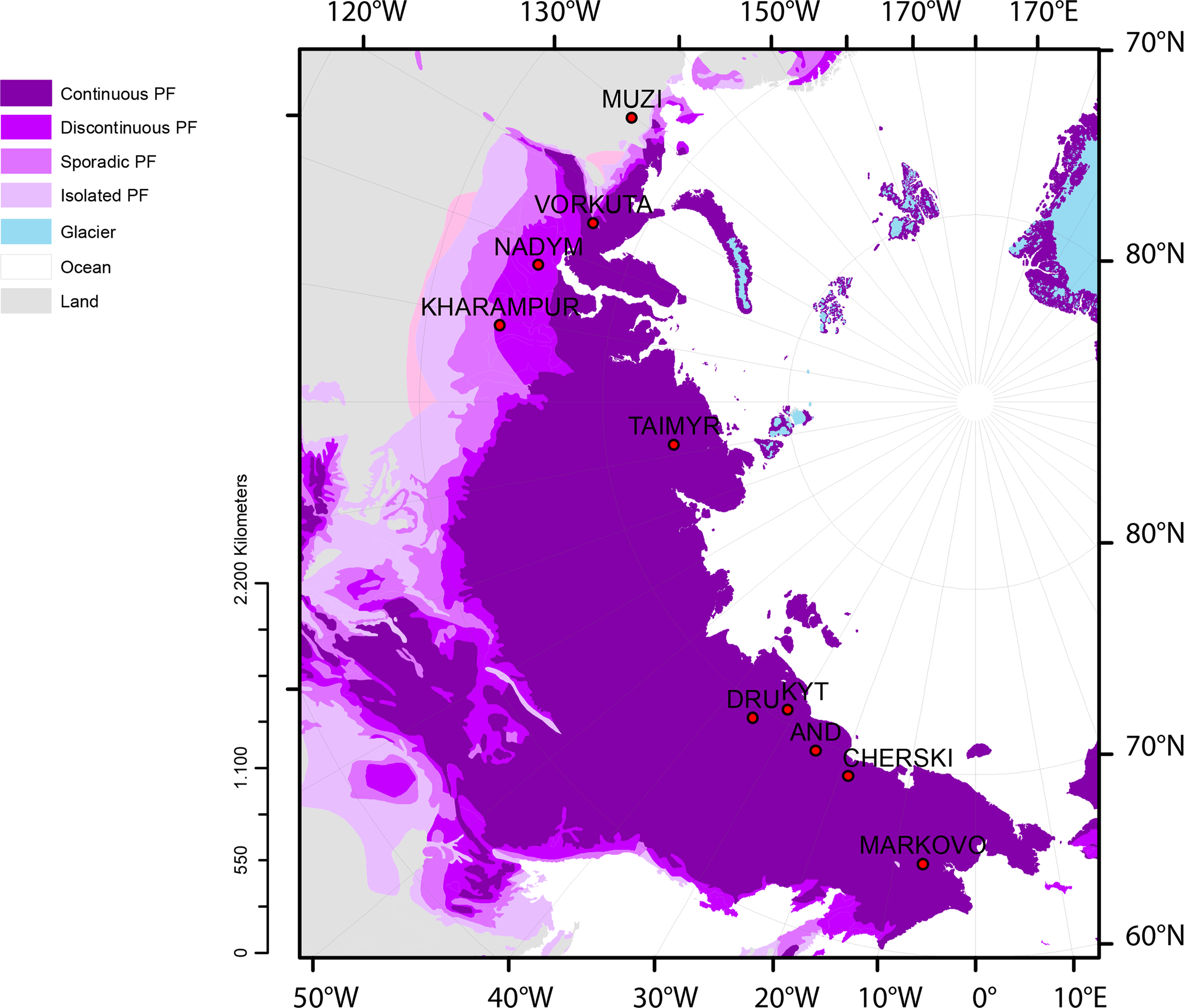
Across Siberia, 10 sites were selected (Figure 1). These sites were chosen in order to represent the diversity of landscapes in the Arctic region and because of their proximity to meteorological stations. Furthermore, among the sites, Kytalyk, Cherski, Vorkuta and Nadym are long-term permafrost monitoring sites [39]. Lastly, an essential criterion for choosing the sites was the ASAR data availability (several acquisitions per month). Kharampur and Vorkuta are underlain by sporadic permafrost and Nadym by discontinuous permafrost, whereas all other sites are underlain by continuous permafrost, with the exception of Muzi, which is not underlain by permafrost [40]. The site locations include lake-rich as well as lake-poor areas. The flat and low altitude areas where the sites are located are generally wet. The Western Siberian Lowlands, the coastal plains and the Taimyr Peninsula largely consist of tundra landscapes with predominating wet conditions (e.g., [41,42]).
2.2. Satellite and in Situ Data
Both the ASCAT and ASAR instruments are active microwave sensors operating in C-band (frequency 5.2 GHz), which is suitable for SSM applications due to the contrasts in dielectric properties between dry and wet soils [24–26]. This forms the basis for SSM retrieval methods from microwave remote sensing. In the method by [8,43], instantaneous backscatter measurements are firstly normalized to a reference incidence angle (40°) and corrected for vegetation influences by making use of the scatterometer multi-incidence angle viewing capacities. The values are thereafter scaled between the so called dry (σ0-dry, 0%) and wet (σ0-wet, 100%) backscatter references, which correspond to the locally obtained historical minimum and maximum backscatter. The resulting soil moisture product is a percentage-index that relates to the uppermost 5 cm of the soil or (in the case of high water content) less. The relative soil moisture is thus calculated as [8,43]:
Since the retrieval algorithm makes use of a change detection technique [12,19] it may be sensitive to other dynamics than those truly related to soil moisture, such as seasonal water body dynamics. In addition, the SSM values can only be derived under unfrozen conditions. Therefore, an algorithm for detecting the surface status and if necessary masking frozen surfaces (creating a surface status flag) has already been implemented for high-latitude applications [17,27]. The ASCAT time series data are available for a predefined discrete global grid (DGG; for definition see [17]). The grid format is based on the assumption that the Earth can be modeled as a rotated ellipsoid. Each grid cell over land is attributed a timeseries of backscatter values which are spatially resampled with an equal spacing of 12.5 km in latitude and longitude. The cells are identified by a unique grid cell index (GPI) [17]. For this study the global original dataset (without temporal aggregation) has been used, except for the model to remotely-sensed data comparison, where a weekly composite of the ASCAT data was used [45]. This specific dataset was developed as requested by users from the global modeling community within the DUE-permafrost project. The weekly composite consists in daily records where the retrieved SSM values from the preceding week are averaged.
The ASAR WS (C-band) dataset has a higher spatial resolution than ASCAT. ASAR was a ScanSAR instrument on board ENVISAT. Its spatial resolution in wide swath (WS) mode is 120 m for all sub-swaths [46]. ASAR had a revisit period of 35 days. Data availability is considerably constraint compared to scatterometer data. Suitable time series can be obtained for a range of locations across Siberia for selected years [47]. For this study, an ASAR WS dataset which was pre-processed over Northern Eurasia for the time period 2007–2008 within the framework of the European Space Agency (ESA) Support To Science Element (STSE) project ALANIS Methane [47–49] was used. Since the backscatter signal decreases with increasing incidence angle of the radar beam relative to the surface, the backscatter measurements are normalized to a common reference angle (30°) using the SAR Geophysical Retrieval Toolbox (SGRT), which is a scripting chain developed by the Institute of Photogrammetry and Remote Sensing (IPF). The scripting chain calls the commercial SARscape or the free NEST software, allowing for the automatization of the entire preprocessing procedure [47,50]. Single images are split up into predefined subsets and stored as time series stacks. In addition, the surface status flag developed for ASCAT [27] is used for masking the frozen ground condition and melting snow from the ASAR data. Point-station data measurements of maximum- and minimum temperature, precipitation and wind speed was obtained from the harmonized Global Summary of the Day and Month Observations dataset from the Global Precipitation Climatology Center [51].
2.3. Land Surface Model
The land surface model ORCHIDEE combines a multi-layer hydrological scheme recently improved for high-latitude processes [35], with a detailed representation of the energy and carbon cycles and the interface between soil and atmosphere. Of more relevance here is the hydrological scheme, which relies on a vertical discretization of the Richards equation allowing for physically-based diffusion of liquid water within the soil, up to a depth of 2 m. Soil freezing, vertical soil compaction and the effect of root water uptake, are also accounted for [52]. When rainfall of meltwater exceed the infiltration capacity of the uppermost soil layers, exceeding water either ponds or flows as surface runoff, depending on the local topography. The model uses as input standard meteorological data (precipitation, air humidity, pressure, temperature, and thermal and solar radiations), which are usually referred to as “forcing data”. It produces several hydrological outputs, including vertically discretized soil moisture content, subsurface and surface runoff and evapotranspiration. The ORCHIDEE land surface model has proven able to reproduce observed hydrological features even in high-latitude regions [36].
The present study uses the model’s output for vertically discretized volumetric SSM of daily resolution. In order to compare the average volumetric soil moisture calculated by the model to the weekly aggregated ASCAT SSM data, a number of adaptations were made. The modeled soil moisture from the uppermost 5 cm of the soil was masked out for frozen conditions and snow cover. For each model grid cell, the local historical maximum and minimum references were found so that the SWI of the model output could be established, rescaling between 0% and 100%. A weekly composite of the model output from the second step was then produced on a daily basis for consistent comparison with the ASCAT high-latitudes product from the DUE-permafrost project (see Sections 2.1 and 2.2) [36]. On average, the agreement between ORCHIDEE SSM and ASCAT SSM, as measured by the daily correlation coefficient of the model and ASCAT weekly composites, is however quite low over our study areas. Possible reasons for this outcome have been mentioned in the introduction.
2.4. Methodology
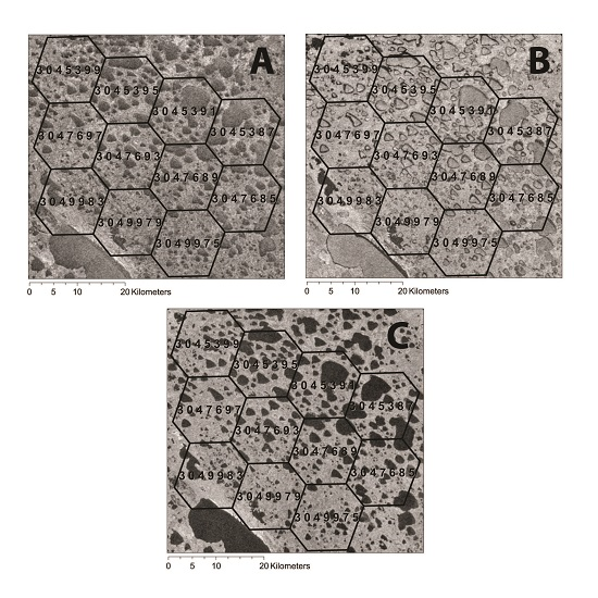
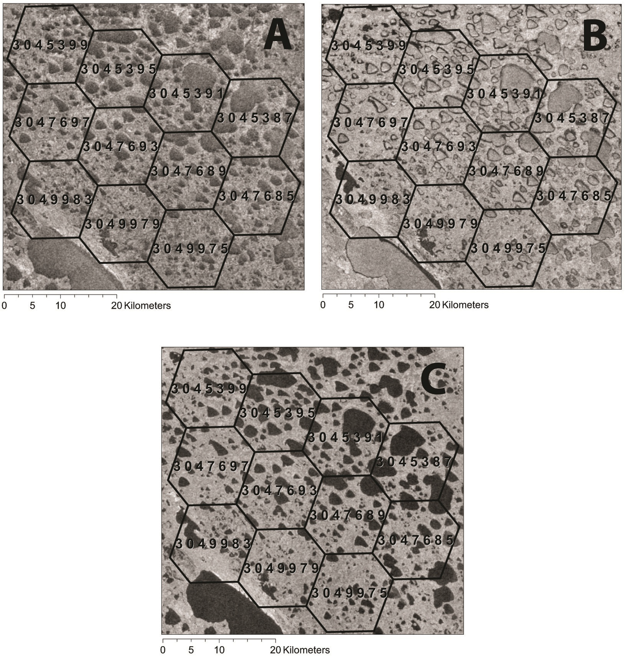
ASCAT SSM time series were retrieved for each DGG cell. For comparability, these DGG extents were used to define regions of interest (ROI) within each ASAR grid stack. For each study site, a 3100 km2 large area was divided into meshes of hexagons using the GPI as center points. This resulted in 9–11 hexagonal ROI within each of the ten sites (Figure 2 shows the 11 ROI in Cherski).
A supervised classification (minimum distance) was performed on ice free ASAR acquisitions with summer maximal lake expansion and water/land contrasts, to separate land from water. Higher backscatter than the typical C-band backscatter for smooth water surfaces may be caused by (1) ice covers on water surfaces and (2) wind and rain action. Wave ripples on the water body surface due to wind and rain increase the surface roughness and hence lead to diffuse scattering and high backscatter values [47,53]. The persistence of lake ice on large lakes well into the summer and the associated water body classification issues have already been pointed out by [47]. To identify any water surface effects, the water areas identified by the classification were replaced by the value −20 dB, which is a typical C-band backscatter value for smooth water surfaces in the used dataset [47,54]. This builds the reference dataset.
The mean backscatter result of the masking and replacement by a reference value, henceforth referred to as refilling, was calculated for each ROI and for each available acquisition. This average from the reference datasets was plotted against the original dataset. The mask effect, , is the difference between the original and the reference ROI average for each available acquisition. The acquisitions were also visually interpreted together with meteorological data in order to identify any rain, ice and wind conditions. In addition to the above described specific examination of the surface effects (potentially from ice, rain and/or wind) it was investigated whether the level of agreement between the ASCAT and ORCHIDEE SSM results could be related to the abundance of lakes. For this purpose, open water fraction and lake size were calculated for each ROI from the ASAR WS data by converting the previously described water classification to polygons. Criteria related to total water cover and lake size were defined and used to separate ROI into three categories:
- (A)
More than 20% lake area per total area including only lakes larger than 10 km2
- (B)
More than 20% lake area per total area including only lakes smaller than 10 km2
- (C)
Less than 20% lake area per total area.
The fractional area of lake, lake count, , ASCAT sensitivity and ASCAT-ORCHIDEE agreement and the correlation thereof, were computed and analysed for each category. Here, the correlation is meant to determine whether significant relationships exist between lake characteristics, identified lake effect on backscatter ( ) and ASCAT SSM retrieval characteristics (sensitivity) or performance (here assessed by the ASCAT-ORCHIDEE agreement). Since ice is assumed more likely to be present in early summer than the high summer months, the during June was calculated separately from that during July-August, to isolate eventual impacts of prevailing ice cover. For the same reason, a two sampled t-test of the from June in relation to that in July-August was done in order to know if there was a significant difference between these two time periods. Analyses of higher temporal resolution than monthly could not be done due to the irregular acquisition intervals by ENVISAT ASAR WS [47].
3. Results
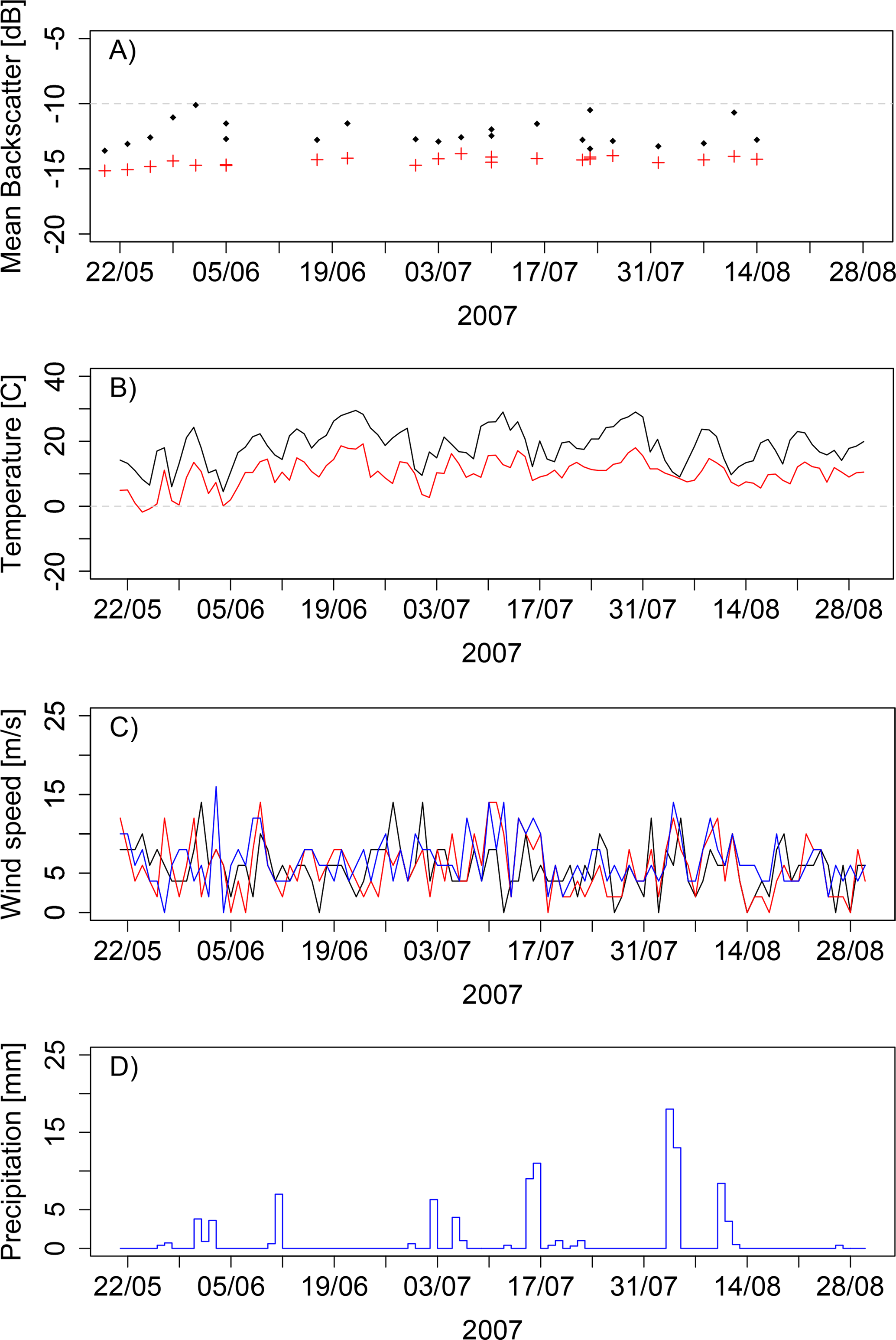
The original mean backscatter for the ROIs is always higher than or equal to the mean backscatter from the reference image since frozen ground conditions and spring snowmelt events have been excluded. Figure 3A shows the backscatter for one of the ROI in Cherski during 2007, including the mean unmasked backscatter (black diamonds) and the mean of the backscatter after having applied the water mask and replaced the backscatter values with the smooth water surface reference value (−20 dB) (red crosses). It can be seen in Figure 3A and that the difference is in the order of more than 2 dB during several occasions during the warm months of the year. Note that the winter months are excluded since ASCAT soil moisture is derived only under unfrozen conditions (see Section 2.2). Figure 3B–D shows the temperature, wind speed and precipitation for the same site and time period.
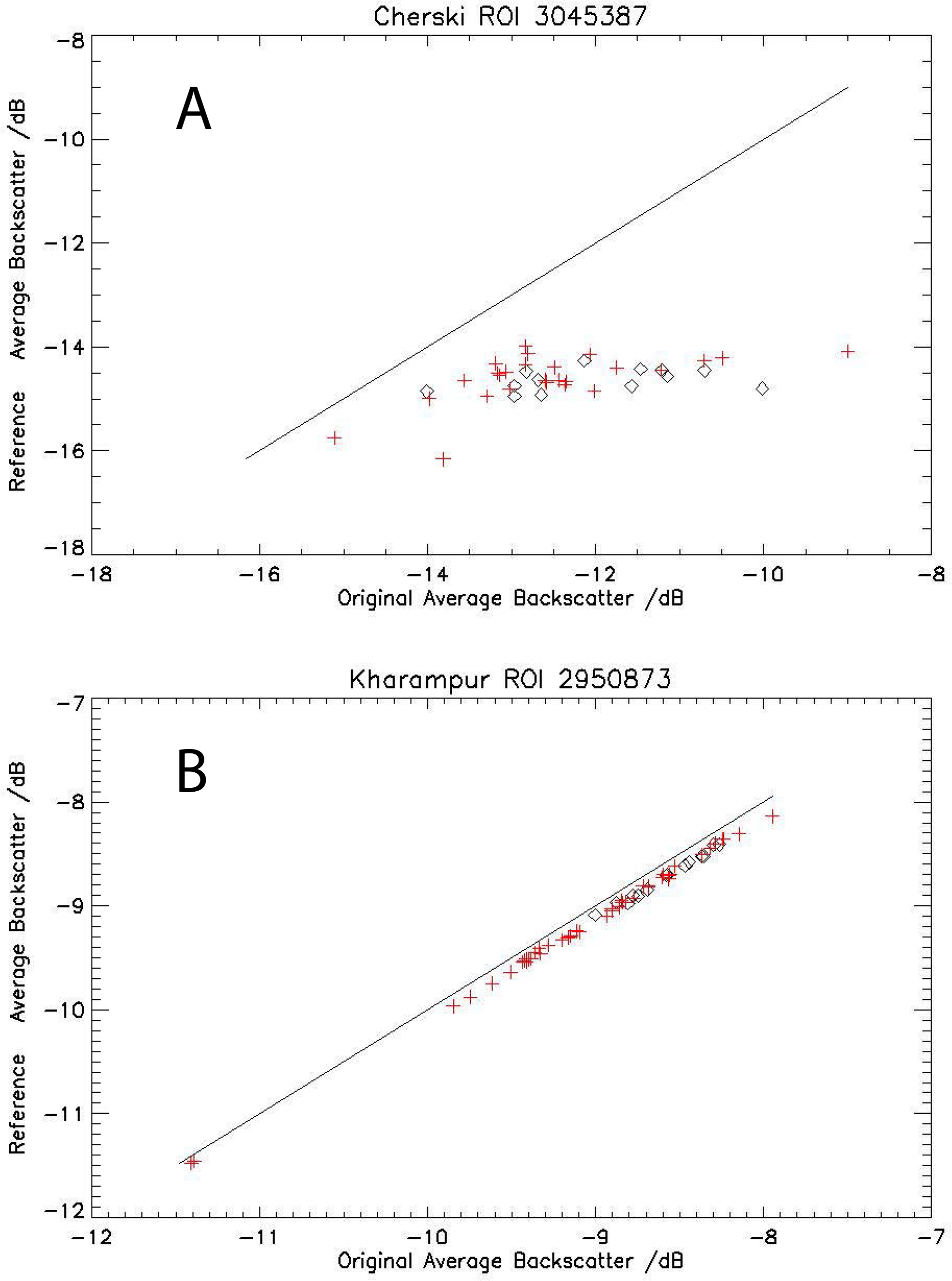
In three of the acquisitions from Cherski in 2007 where was found to be high, either precipitation or high wind speed was identified by visual interpretation of the ASAR data and in the meteorological record. One example is the acquisition from 11 August 2007, illustrated in Figure 2A (see Figure 3D for precipitation data). Figure 2B shows the same area but an acquisition with presumed ice cover. One occasion with presumed prevailing ice cover (17 June 2007) was visually identified for this site during 2007, but strong effects were not recognized compared to the reference (smooth surface). Figure 2C shows relatively smooth water surface conditions for Cherski (6 July 2007), as well as the limits of the hexagonal ROI for this site and their GPI numbers. For Kytalyk, Andryuskino and partly for Druzhina, the results were similar to those from Cherski. In Kharampur, Muzi, Nadym, Taimyr and Vorkuta, is generally low and no significant backscatter change that could be related to weather conditions was observed in the ASAR data. Scatterplots of the reference values as a function of the original data for one of the ROI in Cherski (subject to high ) and one of the ROI in Kharampur (not subject to a high ) are shown in the left and right panel of Figure 4, respectively.
To isolate the potential effect from prevailing ice cover the early summer months are separated from the late summer months: the acquisitions from June are plotted as black diamonds whereas those from July and August as red crosses. Figure 4B shows that the mean from the unmasked backscatter in the case of Kharampur is similar to that of the masked (reference dataset). A clear difference between in the low agreement sites compared to the high agreement sites can be seen. It can not be concluded that is different during the early summer months from the later summer months. When statistically testing the null hypothesis that the is not significantly different in June compared to that in July–August over all ROIs, the p-value is 0.616, which is insufficient for rejecting the hypothesis (regardless if choosing any of the common levels of significance: 0.10, 0.05 or 0.01) and supports our visual analysis.
The extracted data for each ROI, including , lake count, lake area, ASCAT sensitivity and daily correlation with ORCHIDEE from [36] are given in Table 1. This last value is a measure of agreement between the modeled and remotely-sensed surface soil moistures in terms of temporal dynamics. Out of the total 95 ROI, this table includes the 15 ROI with the maximum and the 15 with minimum in June, respectively. Further, Table 2 shows the correlation matrix for the parameters from Table 1, calculated from all the 95 ROI, and separately for the low (including negative high correlation) and the high agreement sites.
For the low agreement sites only (including negative correlation), the sensitivity correlates positively with the total lake area (0.55) and the total number of lakes (0.68) and shows a strong correlation with , in June (0.71) slightly more so than in July–August (0.68). The ASCAT-ORCHIDEE agreement correlates negatively with the sensitivity (−0.68) but, regarding , displays similar agreement in June (−0.53) and in July–August (−0.57). Further, it correlates moderately with the lake area (−0.55) and only weakly with the lake count (−0.30). That is to say, the areas with a low ASCAT-ORCHIDEE agreement correspond to areas with a high water fraction, although they are not linked to a high number of lakes. It is found that the ROI within the lake size group A and B are almost exclusively located within areas of low agreement between the model output and the remote sensing product. This is the case for the majority of the ROI in Andryuskino, Cherski and Druzhina. For Kytalyk, only the ROI with large lakes present are related to low agreement between the model output and remote sensing product. A few ROI within the site Muzi also fall within the group B but the daily correlation here is positive. Muzi contains no lakes but the low seen here is related to the masking out of a river rather than lakes. The ROI within the lake size group A and B also show a strong , ranging from 0.55 to 2.61 dB in the case of group A, from 0.14 to 2.38 for group B, whereas no more than from 0.00 to 0.94 for group C. Lake area is more strongly correlated to the (0.92 in June, 0.91 in July–August) than the lake count is to the (0.46 in June, 0.39 in July–August). Considering the correlation matrix for the high agreement sites, only weak correlation if any at all are found, the caveat being the correlation between lake area and .
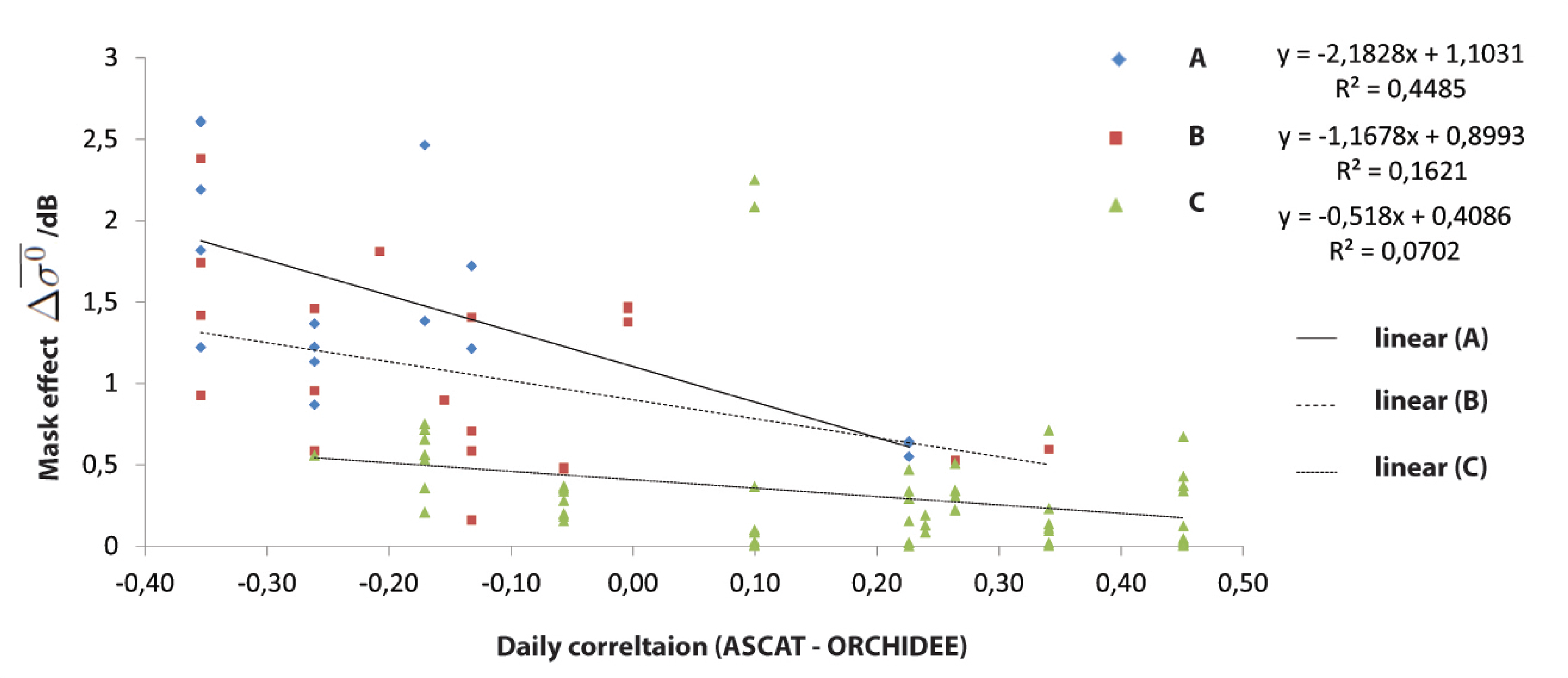
Figure 5 shows from June in dB plotted against the ASCAT-ORCHIDEE agreement. It can be seen that the increases with daily correlation, notably so for group A and B. The R2 can not be said to be strong for any of the groups. However, R2 for group A is notably stronger than both B and C. Results are similar for the two investigated time periods, e.g., June as well as July–August.
4. Discussion
The results confirm that open water surfaces of tundra lakes are typically rough with respect to the used wavelength (C-band). Indeed, authors have previously estimated an on average −4.9 dB higher backscatter (same preprocessing) than under calm conditions [50]. Spatially averaged backscatter deviations for the ROIs which represent the ASCAT cells and include both water and land area reach up to 5 dB. High correspond with times of high wind speed or precipitation. It is here hypothesized that locations with low (including negative) agreement between the ASCAT and ORCHIDEE SSM correspond to areas that have many and/or large lakes and that the at the same locations is high. At sites with positive correlation between ASCAT and the landsurface model SSM (Kharampur, Muzi, Nadym, Taimyr and Vorkuta), is generally low (<0.71 dB). There are two exceptions in Taimyr, where the mask effect is as large as 2.08 and 2.25 dB. These cases correspond to the only ROI in Taimyr with a large total water area (32.44% and 41.17%, respectively). This is however not reflected in the the daily correlation between ASCAT and ORCHIDEE, which is 0.10 for all of the ROI in Taimyr. This could thus be explained by reasons other than water bodies but related to the model, brought up in the Section 2.3.
At Markovo (eastern Siberia), the model-SSM retrieval agreement is low (−0.06). Here, the is less pronounced. It is in fact comparable to the high agreement sites, although the site is located in an area of low agreement. For Markovo, the low agreement between the model output and the ASCAT data could be explained by other reasons than water bodies; it is more likely due to the exceptionally scarce forcing weather data from this part of Siberia [36].
Figure 5 further confirms that there is a difference between the water fraction and lake size classes (groups A, B and C) regarding the dependency of the ASCAT-ORCHIDEE agreement and . Results are similar for the two investigated time periods (June, July-Aug). Although there is some scatter among the categories and the R2 value is moderate, it is found that the magnitude of for group C appears to be independent from the ASCAT-ORCHIDEE correlation whereas it explains 16%–44 % of the variation for group A and B.
At sites with an ASCAT-ORCHIDEE correlation lower than −0.21, the average June ranges from 0.56–2.26 dB. This corresponds to 10%–35% of the overall ASCAT sensitivity to soil moisture, which in turn would translate into as much as 35% higher relative soil moisture value if the difference in ASAR backscatter ( ) would be directly comparable to the ASCAT soil moisture product. For single acquisitions it amounts to 60%–70% in areas of 40%–45% water fraction. A direct comparison to ASCAT backscatter and quantification of impact on soil moisture retrieval is however limited. One would need to make the assumption that the averaged ASAR WS backscatter over the ROI corresponds to the ASCAT backscatter. The hexagonal grid of ROI generated in this study is merely an approximation of the ASCAT grid cells. Furthermore, the absolute backscatter values may deviate due to incidence angle differences (ranging from 25° to 65°) and differences in signal contribution over the footprint for ASCAT [44] as well as actual soil moisture changes. In the cases when the high backscatter events coincide with precipitation events, the impact of dielectric properties changes would need to be taken into account.In the cases when the high backscatter events coincide with precipitation events, the impact of dielectric properties changes would need to be taken into account: it is difficult to separate the backscatter variations due to the actual increase in soil moisture from the action that the rain causes on the surface. Furthermore, it should be considered that the ASCAT dataset which has been used for comparison with ORCHIDEE has been aggregated to weekly time steps. One can expect a smoothing of the backscatter variations in this case, so the actual disagreement with the model may be higher when compared on a daily basis.
For soil moisture retrieval the signal is impacted if the area covered by open water surface within the footprint is large [38]. A surface water fraction flag, derived from the Global Lakes and Wetlands Database [55], exists but it does not take wetland dynamics, temporary inundation and small lakes into account [54]. An improved flag of this kind could be derived from ASAR data [13,56]. Tundra lakes can be considerably smaller than the ASAR WS resolution [57]. The impact of these small lakes would need to be analyzed in addition for the development of a correction algorithm of the scatterometer soil moisture datasets, e.g., by taking into account subpixel-scale fraction of water cover [57].
5. Conclusions
This study examines backscatter variabilities other than related to soil moisture in order to address challenges in radar soil moisture retrieval that are specific for in the Arctic. The impact on the soil moisture retrieval is investigated for sites across Siberia, including permafrost longterm monitoring sites. Satellite derived surface soil moisture datasets would provide valuable additional information to point measurements in these regions. Envisat ASAR WS imaging radar data are investigated in order to identify seasonal variations in backscatter that are not related to SSM but to lake cover surface status. This gives an indication for the magnitude of the impact of such features on the coarser spatial resolution ASCAT SSM retrieval, and cast some light on the model-to-ASCAT low agreement in SSM, highlighted by a previously published study [36]. Different techniques and sensors can be used for SSM retrieval from satellites [7,8,10]. The findings of this study can be applied to systems relying on similar principles: change detection approach in a backscattered signal that is impacted by surface soil moisture but also by surface conditions, e.g., water surface roughness or frozen conditions. Most importantly, these specific findings are applicable to C-band sensors.
Identified backscatter difference is in the order of 2 dB on the mean backscatter over several weeks and up to 5 dB on specific acquisitions in the areas with low ORCHIDEE-ASCAT agreement (no or negative correlation). In comparison, the assumed ASCAT sensitivity for soil moisture changes reaches approximately 7 dB in these areas. A direct translation of the identified difference to deviations of the soil moisture values from the actual values would need to take sensor and data processing differences into account.
Regions with high backscatter deviations (averaged over ASCAT grid cell) from the reference dataset representing smooth water surfaces ( ) are however evidently characterized by a high percentage of total lake area, i.e., many of the ROI in eastern Siberia: Cherski, Andryuskio, Druzhina and Kytalyk. The sites Kharampur, Taimyr, Nadym, Vorkuta and Muzi (western and central Siberia), show low and are areas with few lakes. In the case of Markovo (far eastern Siberia) the low agreement between the model output and the SSM product is more likely explained by the exceptionally scarce weather data from this area used to force the model [36]. Although events of wind and precipitation identified by the meteorological data only occurred infrequently for each site, the correlation between the backscatter deviation and the ASCAT-ORCHIDEE agreement together with the lake size distribution lead to the conclusion that water body fraction and water body size is one explanation for the disagreement between the ASCAT and ORCHIDEE SSM. In this context, it should be considered that the ORCHIDEE model does not represent ephemeral lakes (i.e., normally dry lakes that fills with water for short periods), which are an additional source of error for ORCHIDEE in lake-rich areas.
The low and negative correlation sites compared to the high agreement sites clearly show different results for the in relation to the total lake expansion and size distribution. However, no significant difference was shown between the early and late summer months. The presence of ice cover on lakes does not give strong effect on the in this study.
In addition to the above and other model-related issues as discussed by [36], the low agreement between ORCHIDEE and ASCAT SSM in the Siberian lowlands is likely related to the existence of water bodies. Therefore, it should be noted that in circumpolar lowland permafrost areas, where ponds and lakes are common features, the presence of water bodies has an impact on the ASCAT SSM retrieval. This supports what has previously been pointed out about open water having a disturbing influence on the signal and thus for the surface soil moisture retrieval if the area covered by open water surface within the footprint is large [38]. In Siberia, an improved surface flag product that takes into account wetland dynamics could be derived from Synthetic Aperture Radar (SAR) imagery [32,53]. The usage of higher spatial resolution data for SSM retrieval as available from Sentinel-1 is required in regions with large water fractions, including lowland permafrost environments.
Acknowledgments
The authors acknowledge financial support by the European Union FP7-ENV project PAGE21 (Changing Permafrost in the Arctic and its Global effects in the 21st century) under contract No. GA282700. The ALANIS project was funded by the European Space Agency (ESA) Support to Science Element (STSE) program (ESRIN Contr. No. 4000100647/10/I-LG).
Author Contributions
All co-authors have substantially contributed to the writing of the manuscript. In addition, Elin Högström has carried out all analyses and prepared the first draft. Anna Maria Trofaier has set the study into a wider context including SAR applications, took care of layout and provided native English editing. All items related to land surface modelling have been prepared by Isabella Gouttevin. Annett Bartsch developed the concept for the study and provided expertise in EO data handling.
Conflicts of Interest
The authors declare no conflict of interest.
References
- IPCC. Observations: Cryosphere. Proceedings of the Climate Change 2013: The Physical Science Basis. Contribution of Working Group I to the Fifth Assessment Report of the Intergovernmental Panel on Climate Change, Stockholm, Sweden, 23–26 September 2013; pp. 362–364.
- Friborg, T.; Soegaard, H.; Christensen, T.; Lloyd, C.; Panikov, N. Siberian wetlands: Where a sink is a source. Geophys. Res. Lett 2004, 30. [Google Scholar] [CrossRef]
- Christensen, T.R.; Johansson, T.R.; Akerman, H.J.; Mastepanov, M.; Malmer, N.; Friborg, T.; Crill, P.; Svensson, B H. Thawing sub-arctic permafrost: Effects on vegetation and methane emissions. Geophys. Res. Lett 2004, 31. [Google Scholar] [CrossRef]
- Langer, M.; Westermann, S.; Heikenfeld, M.; Dorn, W.; Boike, J. Satellite-based modeling of permafrost temperatures in a tundra lowland landscape. Remote Sens. Environ 2013, 135, 12–24. [Google Scholar]
- Swenson, S.; Lawrence, D.; Lee, H. Improved simulation of the terrestrial hydrological cycle in permafrost regions by the Community Land Model. J. Adv. Model. Earth Syst 2012, 4. [Google Scholar] [CrossRef]
- Lupascu, M.; Welker, J.; Seibt, U.; Maseyk, K.; Xu, X.; Czimczik, C. High Arctic wetting reduces permafrost carbon feedbacks to climate warming. Nat. Clim. Chang 2013, 4, 51–55. [Google Scholar]
- Kimball, J.S.; Jones, L.A.; Zhang, K.; Heinsch, F.A.; McDonald, K.C.; Oechel, W.C. A satellite approach to estimate land—Atmosphere exchange for boreal and arctic biomes using MODIS and AMSR-E. IEEE Trans. Geosci. Remote Sens 2009, 47, 569–587. [Google Scholar]
- Wagner, W.; Noll, J.; Borgeaud, M.; Rott, H. Monitoring soil moisture over the Canadian prairies with the ERS scatterometer. IEEE Trans. Geosci. Remote Sens 1999, 37, 206–216. [Google Scholar]
- Naeimi, V.; Bartalis, Z.; Wagner, W. ASCAT soil moisture: An assessment of the data quality and consistency with the ERS scatterometer heritage. J. Hydrometeorol 2009, 10, 555–563. [Google Scholar]
- Njoku, E.G.; Jackson, T.J.; Lakshmi, V.; Chan, T.K.; Nghiem, S.V. Soil moisture retrieval from AMSR-E. IEEE Trans. Geosci. Remote Sens 2003, 41, 215–229. [Google Scholar]
- Koike, T.; Nakamura, Y.; Kaihotsu, I.; Davva, G.; Matsuura, N.; Tamagawa, K.; Fujii, H. Development of an Advanced Microwave Scanning Radiometer (AMSR-E) algorithm of soil moisture and vegetation water content. Annu. J. Hydraul. Eng. JSCE 2004, 48, 217–222. [Google Scholar]
- Wagner, W.; Bloschl, G.; Pampaloni, P.; Calvet, J.C.; Bizzarri, B.; Wigneron, J.P.; Kerr, Y. Operational readiness of microwave remote sensing of soil moisture for hydrologic applications. Nord. Hydrol 2007, 38, 1–20. [Google Scholar]
- Bartsch, A.; Balzter, H.; George, C. The influence of regional surface soil moisture anomalies on forest fires in Siberia observed from satellites. Environ. Res. Lett 2009, 4. [Google Scholar] [CrossRef]
- Künzer, C.; Zhao, D.; Scipal, K.; Sabel, D.; Naeimi, V.; Bartalis, Z.; Hasenauer, S.; Mehl, H.; Dech, S.; Wagner, W. El Niño influences represented in ERS scatterometer derived soil moisture data. Appl. Geogr 2009, 29, 463–477. [Google Scholar]
- Paulik, C.; Dorigo, W.; Wagner, W.; Kidd, R. Validation of the ASCAT soil water index using in situ datafrom the international soil moisture network. Int. J. Appl. Earth Obs. Geoinf 2014, 30, 1–8. [Google Scholar]
- Brocca, L.; Melone, F.; Moramarco, T.; Wagner, W.; Hasenauer, S. ASCAT soil wetness index validation through in situ and modeled soil moisture data in central Italy. Remote Sens. Environ 2010, 114, 2745–2755. [Google Scholar]
- Naeimi, V.; Scipal, K.; Bartalis, Z.; Hasenauer, S.; Wagner, W. An improved soil moisture retrieval algorithm for ERS and METOP scatterometer observations. IEEE Trans. Geosci. Remote Sens 2009, 47, 1999–2013. [Google Scholar]
- Albergel, C.; de Rosnay, P.; Gruhier, C.; Muñoz-Sabater, J.; Hasenauer, S.; Isaksen, L.; Kerr, Y.; Wagner, W. Evaluation of remotely sensed and modelled soil moisture products using global ground-based in situ observations. Remote Sens. Environ 2012, 118, 215–226. [Google Scholar]
- Wagner, W.; Pathe, C.; Doubkova, M.; Sabel, D.; Bartsch, A.; Hasenauer, S.; Blöschl, G.; Scipal, K.; Martínez-Fernández, J.; Löw, A. Temporal stability of soil moisture and radar backscatter observed by the Advanced Synthetic Aperture Radar (ASAR). Sensors 2008, 8, 1174–1197. [Google Scholar]
- Doubkova, M.; van Dijk, A.I.J.M.; Sabel, D.; Wagner, W.; Blöschl, G. Evaluation of the predicted error of the soil moisture retrieval from C-band SAR by comparison against modelled soil moisture estimates over Australia. Remote Sens. Environ 2012, 120, 188–196. [Google Scholar]
- Bartsch, A.; Sabel, D.; Wagner, W.; Park, S.E. Considerations for derivation and use of soil moisture data from active microwave satellites at high latitudes. Proceedings of the 2011 IEEE International Geoscience and Remote Sensing Symposium (IGARSS), Vancouver, BC, Canada, 24–29 July 2011; pp. 3132–3135.
- Ulaby, F.T.; Moore, R.K.; Fung, A.K. Microwave Remote Sensing, Active and Passive, III, Radar Remote Sensing and Surface Scattering and Emission Theory; Artech House Publishers: London, UK/Boston, MA, USA, 1986. [Google Scholar]
- Scipal, K.; Drusch, M.; Wagner, W. Assimilation of a ERS scatterometer derived soil moisture index in the ECMWF numerical weather prediction system. Adv. Water Resour 2008, 31, 1101–1112. [Google Scholar]
- Ulaby, F.T.; Moore, R.K.; Fung, A.K. Microwave Remote Sensing, Active and Passive, II, Radar Remote Sensing and Surface Scattering and Emission Theory; Artech House Publishers: London, UK/Boston, MA, USA, 1982. [Google Scholar]
- Way, J.; Zimmermann, R.; Rignot, E.; McDonald, K.; Oren, R. Winter and spring thaw as observed with imaging radar at BOREAS. J. Geophys. Res. Atmos. (1984–2012) 1997, 102, 29673–29684. [Google Scholar]
- Wegmüller, U. The effect of freezing and thawing on the microwave signatures of bare soil. Remote Sens. Environ 1990, 33, 123–135. [Google Scholar]
- Naeimi, V.; Paulik, C.; Bartsch, A.; Wagner, W.; Kidd, R.; Park, S.E.; Elger, K.; Boike, J. ASCAT Surface State Flag (SSF): Extracting information on surface freeze/thaw conditions from backscatter data using an empirical threshold-analysis algorithm. IEEE Trans. Geosci. Remote Sens 2012, 50, 2566–2582. [Google Scholar]
- Bartsch, A. Ten years of SeaWinds on QuikSCAT for snow applications. Remote Sens 2010, 2, 1142–1156. [Google Scholar]
- Bartsch, A.; Kidd, R.A.; Wagner, W.; Bartalis, Z. Temporal and spatial variability of the beginning and end of daily spring freeze/thaw cycles derived from scatterometer data. Remote Sens. Environ 2007, 106, 360–374. [Google Scholar]
- Entekhabi, D.; Njoku, E.G.; O’Neill, P.E.; Kellogg, K.H.; Crow, W.T.; Edelstein, W.N.; Entin, J.K.; Goodman, S.D.; Jackson, T.J.; Johnson, J.; et al. The soil moisture active passive (SMAP) mission. IEEE Proc 2010, 98, 704–716. [Google Scholar]
- Brocca, L.; Moramarco, T.; Melone, F.; Wagner, W.; Hasenauer, S.; Hahn, S. Assimilation of surface- and root-zone ASCAT soil moisture products into rainfall-runoff modeling. IEEE Trans. Geosci. Remote Sens 2012, 50, 2542–2555. [Google Scholar]
- Schumann, G.; Bates, P.D.; Horritt, M.S.; Matgen, P.; Pappenberger, F. Progress in integration of remote sensing—Derived flood extent and stage data and hydraulic models. Rev. Geophys 2009, 47. [Google Scholar] [CrossRef]
- Woo, M.K.; Kane, D.L.; Carey, S.K.; Yang, D. Progress in permafrost hydrology in the new millennium. Permafr. Periglac. Process 2008, 19, 237–254. [Google Scholar]
- Marchenko, S.; Romanovsky, V.; Tipenko, G. Numerical modeling of spatial permafrost dynamics in Alaska. Proceedings of the Ninth International Conference on Permafrost, Institute of Northern Engineering, University of Alaska Fairbanks, Fairbanks, AK, USA, 29 June–3 July 2008; 29, pp. 1125–1130.
- Gouttevin, I.; Krinner, G.; Ciais, P.; Polcher, J.; Legout, C. Multi-scale validation of a new soil freezing scheme for a land-surface model with physically-based hydrology. Cryosphere 2012, 6, 407–430. [Google Scholar]
- Gouttevin, I.; Bartsch, A.; Krinner, G.; Naeimi, V. A comparison between remotely-sensed and modelled surface soil moisture (and frozen status) at high latitudes. Hydrol. Earth Syst. Sci. Discuss 2013, 10. [Google Scholar] [CrossRef]
- Wismann, V. Monitoring of seasonal thawing in Siberia with ERS scatterometer data. IEEE Trans. Geosci. Remote Sens 2000, 38, 1804–1809. [Google Scholar]
- Wagner, W.; Hahn, S.; Kidd, R.; Melzer, T.; Bartalis, Z.; Hasenauer, S.; Figa-Saldaña, J.; de Rosnay, P.; Jann, A.; Schneider, S.; et al. The ASCAT soil moisture product: A review of its specifications, validation results, and emerging applications. Meteorol. Z 2013, 22, 5–33. [Google Scholar]
- Romanovsky, V.E.; Smith, S.L.; Christiansen, H.H. Permafrost thermal state in the polar Northern Hemisphere during the international polar year 2007–2009: A synthesis. Permafr. Periglac. Process 2010, 21, 106–116. [Google Scholar]
- Brown, J.; Ferrians, O.J.; Heginbottom, J.; Melnikov, E. Circum-Arctic Map of Permafrost and Ground-Ice Conditions, National Snow and Ice Data Center; Digital Media. Available online: http://nsidc.org/data/docs/fgdc/ggd318_map_circumarctic/ (accessed on 17 September 2014).
- Serreze, M.C.; Etringer, A.J. Precipitation characteristics of the Eurasian Arctic drainage system. Int. J. Climatol 2003, 23, 1267–1291. [Google Scholar]
- Boike, J.; Wille, C.; Abnizova, A. Climatology and summer energy and water balance of polygonal tundra in the Lena River Delta, Siberia. J. Geophys. Res. Biogeosci. (2005–2012) 2008, 113. [Google Scholar] [CrossRef]
- Wagner, W.; Lemoine, G.; Borgeaud, M.; Rott, H. A study of vegetation cover effects on ERS scatterometer data. IEEE Trans. Geosci. Remote Sens 1999, 37, 938–948. [Google Scholar]
- Bartalis, Z.; Wagner, W.; Naeimi, V.; Hasenauer, S.; Scipal, K.; Bonekamp, H.; Figa, J.; Anderson, C. Initial soil moisture retrieval from the METOP—A Advanced Scatterometer (ASCAT). Geophys. Res. Lett 2007, 34. [Google Scholar] [CrossRef]
- Paulik, C.; Melzer, T.; Hahn, S.; Bartsch, A.; Heim, B.; Elger, K.; Wagner, W. Circumpolar Surface Soil Moisture and Freeze/Thaw Surface Status Remote Sensing Products (Version 2) with Links to Geotiff Images and NetCDF Files (2007-01 to 2010-09); TU Vienna: Vienna, Austria, 2012. [Google Scholar]
- Closa, J.; Rosich, B.; Monti-Guarnieri, A. The ASAR wide swath mode products. Proceedings of the 2003 IEEE International Geoscience and Remote Sensing Symposium (IGARSS’03), Toulouse, France, 21–25 July 2003; 2, pp. 1118–1120.
- Bartsch, A.; Trofaier, A.; Hayman, G.; Sabel, D.; Schlaffer, S.; Clark, D.; Blyth, E. Detection of open water dynamics with ENVISAT ASAR in support of land surface modelling at high latitudes. Biogeosciences 2012, 9, 703–714. [Google Scholar]
- Reschke, J.; Bartsch, A.; Schlaffer, S.; Schepaschenko, D. Capability of C-Band SAR for operational wetland monitoring at high latitudes. Remote Sens 2012, 4, 2923–2943. [Google Scholar]
- Trofaier, A.; Bartsch, A.; Rees, W.; Leibman, M. Assessment of spring floods and surface water extent over the Yamalo-Nenets Autonomous District. Environ. Res. Lett 2013, 8. [Google Scholar] [CrossRef]
- Sabel, D.; Bartsch, A.; Schlaffer, S.; Klein, J.P.; Wagner, W. Soil moisture mapping in permafrost regions—An outlook to Sentinel-1. Proceedings of the 2012 IEEE International Geoscience and Remote Sensing Symposium (IGARSS), Munich, Germany, 22–27 July 2012; pp. 1216–1219.
- Climate Prediction Center/National Centers for Environmental Prediction/National Weather Service/NOAA/U.S. Dpt. of Commerce. 1987, Updated Half-Yearly. CPC Global Summary of Day/Month Observations, 1979-Continuing. Research Data Archive at the National Center for Atmospheric Research, Computational and Information Systems Laboratory. Dataset. Available online: http://rda.ucar.edu/datasets/ds512.0/ (accessed on 27 July 2011).
- de Rosney, P.; Polcher, J. Modelling root water uptake in a complex land surface scheme coupled to a GCM. Hydrol. Earth Syst. Sci 1998, 2, 239–255. [Google Scholar]
- Bartsch, A.; Wagner, W.; Scipal, K.; Pathe, C.; Sabel, D.; Wolski, P. Global monitoring of wetlands—The value of ENVISAT ASAR Global mode. J. Environ. Manag 2009, 90, 2226–2233. [Google Scholar]
- Bartsch, A.; Pathe, C.; Wagner, W.; Scipal, K. Detection of permanent open water surfaces in central Siberia with ENVISAT ASAR wide swath data with special emphasis on the estimation of methane fluxes from tundra wetlands. Hydrol. Res 2008, 39, 89–100. [Google Scholar]
- Lehner, B.; Döll, P. Development and validation of a global database of lakes, reservoirs and wetlands. J. Hydrol 2004, 296, 1–22. [Google Scholar]
- Schumann, G.; Lunt, D.; Valdes, P.; de Jeu, R.; Scipal, K.; Bates, P. Assessment of soil moisture fields from imperfect climate models with uncertain satellite observations. Hydrol. Earth Syst. Sci 2009, 13, 1545–1553. [Google Scholar]
- Muster, S.; Langer, M.; Heim, B.; Westermann, S.; Boike, J. Subpixel heterogeneity of ice-wedge polygonal tundra: A multi-scale analysis of land cover and evapotranspiration in the Lena River Delta, Siberia. Tellus B 2012, 64. [Google Scholar] [CrossRef]


| Site Name | GPI | June Δ (dB) | July–August Δ (dB) | Lake | Sensitivity Mean (dB) | Daily Correlation | |||||
|---|---|---|---|---|---|---|---|---|---|---|---|
| Min | Max | Mean | Min | Max | Mean | Count | Area (%) | ||||
| CHE | 3045387 | 0.85 | 4.78 | 2.61 | 1.01 | 5.09 | 2.44 | 34 | 44.84 | 7.29 | −0.35 |
| CHE | 3045391 | 0.41 | 4.62 | 2.60 | 0.67 | 4.50 | 2.22 | 36 | 40.82 | 7.49 | −0.35 |
| KYT | 3084867 | 1.43 | 4.16 | 2.46 | 1.09 | 3.98 | 2.46 | 12 | 39.48 | 6.27 | −0.17 |
| CHE | 3045395 | 0.69 | 4.25 | 2.38 | 0.02 | 4.05 | 1.80 | 35 | 41.83 | 7.08 | −0.35 |
| TAI | 3120067 | 0.94 | 4.12 | 2.25 | 0.42 | 3.85 | 2.97 | 3 | 41.17 | 5.22 | 0.10 |
| CHE | 3047693 | 1.96 | 2.37 | 2.19 | 1.46 | 2.45 | 1.95 | 27 | 23.84 | 7.65 | −0.35 |
| TAI | 3118181 | 0.83 | 3.53 | 2.08 | 0.38 | 3.33 | 2.70 | 1 | 32.44 | 6.01 | 0.10 |
| CHE | 3047689 | 0.49 | 3.21 | 1.82 | 0.59 | 3.53 | 1.66 | 41 | 32.19 | 7.73 | −0.35 |
| CHE | 3047685 | 0.21 | 3.33 | 1.81 | 0.49 | 4.01 | 1.70 | 42 | 31.99 | 7.85 | −0.21 |
| CHE | 3047697 | 1.54 | 1.88 | 1.74 | 1.31 | 2.06 | 1.59 | 35 | 17.26 | 6.89 | −0.35 |
| AND | 3049899 | 0.62 | 2.60 | 1.72 | 0.36 | 2.05 | 1.19 | 43 | 23.83 | 6.06 | −0.13 |
| AND | 3052177 | 0.49 | 2.24 | 1.47 | 0.05 | 1.91 | 1.01 | 27 | 23.44 | 5.89 | 0.00 |
| DRU | 3033509 | 0.21 | 2.92 | 1.46 | 0.47 | 2.85 | 1.28 | 22 | 18.91 | 5.74 | −0.26 |
| AND | 3047609 | 0.61 | 2.32 | 1.46 | 0.41 | 1.86 | 1.08 | 45 | 22.26 | 6.36 | 0.00 |
| CHE | 3045399 | 0.38 | 2.25 | 1.42 | 0.20 | 2.35 | 1.04 | 45 | 30.09 | 6.41 | −0.35 |
| KHA | 2948131 | 0.00 | 0.01 | 0.01 | 0.01 | 0.01 | 0.01 | 0 | 0.00 | 5.26 | 0.34 |
| TAI | 3120063 | 0.00 | 0.01 | 0.00 | 0.00 | 0.01 | 0.00 | 0 | 0.00 | 5.18 | 0.10 |
| KHA | 2945369 | 0.00 | 0.00 | 0.00 | 0.00 | 0.01 | 0.00 | 0 | 0.00 | 5.40 | 0.34 |
| VOR | 3013089 | 0.00 | 0.00 | 0.00 | 0.00 | 0.00 | 0.00 | 5 | 0.61 | 5.91 | 0.45 |
| MUZ | 2961321 | 0.00 | 0.00 | 0.00 | 0.00 | 0.00 | 0.00 | 0 | 0.00 | 4.50 | 0.23 |
| Low Agreement Sites | ||||||
| Lake count | Lake area | Sensitivity | June | July–August | Daily correlation | |
| Lake count | *** | *** | *** | ** | ||
| Lake area | *** | *** | *** | *** | ||
| Sensitivity | 0.55 | 0.68 | *** | *** | *** | |
| June | 0.46 | 0.92 | 0.71 | *** | ||
| July–August | 0.39 | 0.91 | 0.68 | *** | ||
| Daily correlation | −0.30 | −0.55 | −0.68 | −0.53 | −0.57 | |
| High Agreement Sites | ||||||
| Lake count | Lake area | Sensitivity | June | July–August | Daily correlation | |
| Lake count | | | | | | | | | ||
| Lake area | | | *** | *** | | | ||
| Sensitivity | 0.03 | −0.04 | | | | | | | |
| June | 0.16 | 0.97 | 0.00 | | | ||
| July–August | 0.10 | 0.96 | 0.00 | | | ||
| Daily correlation | 0.01 | −0.25 | 0.38 | −0.25 | −0.30 | |
|= p-value insufficient; bold = strong correlation; italic = moderate correlation;**= p-value < 0.01;***= p-value < 0.001.
© 2014 by the authors; licensee MDPI, Basel, Switzerland This article is an open access article distributed under the terms and conditions of the Creative Commons Attribution license (http://creativecommons.org/licenses/by/3.0/).
Share and Cite
Högström, E.; Trofaier, A.M.; Gouttevin, I.; Bartsch, A. Assessing Seasonal Backscatter Variations with Respect to Uncertainties in Soil Moisture Retrieval in Siberian Tundra Regions. Remote Sens. 2014, 6, 8718-8738. https://doi.org/10.3390/rs6098718
Högström E, Trofaier AM, Gouttevin I, Bartsch A. Assessing Seasonal Backscatter Variations with Respect to Uncertainties in Soil Moisture Retrieval in Siberian Tundra Regions. Remote Sensing. 2014; 6(9):8718-8738. https://doi.org/10.3390/rs6098718
Chicago/Turabian StyleHögström, Elin, Anna Maria Trofaier, Isabelle Gouttevin, and Annett Bartsch. 2014. "Assessing Seasonal Backscatter Variations with Respect to Uncertainties in Soil Moisture Retrieval in Siberian Tundra Regions" Remote Sensing 6, no. 9: 8718-8738. https://doi.org/10.3390/rs6098718