Restoration of Simulated EnMAP Data through Sparse Spectral Unmixing

Abstract

This paper proposes the use of spectral unmixing and sparse reconstruction methods to restore a simulated dataset for the Environmental Mapping and Analysis Program (EnMAP), the forthcoming German spaceborne hyperspectral mission. The described method independently decomposes each image element into a set of representative spectra, which come directly from the image and have previously undergone a low-pass filtering in noisy bands. The residual vector from the unmixing process is considered as mostly composed of noise and ignored in the reconstruction process. The first assessment of the results is encouraging, as the original bands taken into account are reconstructed with a high signal-to-noise ratio and low overall distortions. Furthermore, the same method could be applied for the inpainting of dead pixels, which could affect EnMAP data, especially at the end of the satellite’s life cycle.

1. Introduction

The future EnMAP (Environmental Mapping and Analysis Program) mission will be able to acquire images at $\pm 30$ off-nadir to achieve revisit times of up to four days. The different acquisition angles, coupled with variations in illumination conditions, will introduce considerable variations in the signal-to-noise ratio (SNR) across the spectral bands and will hinder the analysis of the images, especially in some spectral ranges and for targets characterized by a low surface albedo. Furthermore, the system could experience a degradation in performance of the sensor’s electronics, introducing up to 1% of dead pixels into the acquired images. Therefore, the future EnMAP data could benefit from denoising and inpainting techniques with a high degree of automation.

A denoising technique based on spectral unmixing [1], unmixing-based denoising (UBD), has been recently proposed to selectively retrieve corrupted spectral bands by exploiting their correlation with non-corrupted pixels across the whole spectral dimension [2]. Of particular interest is that UBD has been also successfully applied to restore dead pixels and corrupted values in hyperspectral datasets in [3], with no change in settings. Therefore, it would be desirable to apply this method to improve the forthcoming EnMAP products. This paper proposes sparse unmixing-based denoising (SUBD), a modified version of UBD relying on sparse reconstruction techniques, which have been shown to outperform traditional unmixing approaches [4].

For a remotely-sensed image acquired at typical spatial resolutions, the underlying assumption of sparse spectral unmixing is that only a limited number of pure materials can contribute to the backscattered energy measured in a single resolution cell. Accordingly, these methods are able to decompose the spectrum of each pixel in fractions related to only a few reference spectra. Furthermore, the selection can be done from an overcomplete spectral library, i.e., a collection of spectra with a dimensionality higher than the number of bands in the dataset [4,5,6]. This is in turn achieved by solving optimization problems, such as basis pursuit denoising (BPDN) [7] or least absolute shrinkage and selection operator (LASSO) [8]. As the name implies, BPDN is a denoising algorithm, which approximates a noisy signal with entries from a wavelet dictionary, minimizing the number of wavelets used in the process, and considering the rest of the contributions to the signal as noise.

Sparse reconstruction is coupled with UBD by selecting as overcomplete spectral library a large set of pixels randomly selected from the image and preprocessed in order to present reduced noise contributions. Through UBD, the full spectral information of each image element can be exploited, combining the denoising properties of BPDN with the use of a library composed of real spectra, as in a traditional sparse unmixing problem. Weighting parameters are set across the whole spectral range in order to derive most of the information for the reconstruction of a given noisy band from other correlated bands.

The first results are presented on a noisy synthetic EnMAP dataset in which the proposed algorithm is able to successfully restore the corrupted band of interest. The method can be run with the same settings also to successfully perform inpainting of dead pixels in the same spectral band. Comparisons with the state of the art in terms of similarity to a model noise-free image suggest that the proposed technique could offer a viable solution to restore EnMAP images acquired in unfavorable conditions, also for its high degree of automation.

The paper is structured as follows. Section 2 introduces the EnMAP mission, focusing on the potential benefits of a restoration procedure applied to the acquired images. Section 3 gives a brief reminder of UBD, while Section 4 discusses the advantages of sparse reconstruction methods and describes how to use them to increase the degree of automation of UBD and to improve its results. Section 5 reports some experiments on denoising of bands with low SNR for a simulated EnMAP hyperspectral dataset, while in Section 6 dead pixel inpainting on the same dataset using the same technique is carried out. Section 7 contains conclusions.

2. Signal-to-Noise Ratio and Dead Pixels in EnMAP

EnMAP is a German, Earth-observing, imaging spectroscopy, spaceborne mission planned for launch in 2018 and with a lifetime of five years [9]. The HSI (hyperspectral imager) will consist of two push broom imaging spectrometers: one for the VNIR (visible and near infrared) spectral range from 420 to 1000 nm with a sampling distance of 6.5 nm and one for the SWIR (shortwave infrared) spectral range from 900 to 2450 nm with a sampling distance of 10 nm. The ground pixel size will remain constant at a certain latitude, i.e., 30 m × 30 m at nadir at 48 northern latitude. With 1000 valid pixels, this yields a swath width of 30 km. One of the key system performance parameters is the SNR (in this paper considered as the power ratio between signal and background noise). Figure 1 illustrates the predicted performance for SNR at the sensors for nadir observations under three different conditions and for a 10-nm equivalent bandwidth [10].

Figure 1. Predicted performances for EnMAP’s SNR in the visual to near-infrared (VNIR) and short wave infrared (SWIR) spectral ranges, courtesy of OHB System AG [10].

Figure 1. Predicted performances for EnMAP’s SNR in the visual to near-infrared (VNIR) and short wave infrared (SWIR) spectral ranges, courtesy of OHB System AG [10].

Thus, even if the SNR is predicted to be high, for situations of low surface albedo or Sun zenith angle, it will be reduced, and methods for denoising of hyperspectral images become essential.

A decrease in SNR is only one of the data corruption sources, as especially at the end of the mission’s life cycle, EnMAP data could be additionally corrupted by a non-negligible amount of dead pixels. Dead pixels of the focal plane arrays (FPA) are defined as pixels with permanently no physical meaning, e.g., no response (cold pixels), saturated pixels even at small radiance input (hot pixels), high amplitude variations compared to neighboring pixel values (flickering pixels) or constant pixel values at changing input radiances. As a dead pixel mask is known and determined pre-launch by laboratory measurements and updated during in-flight calibration and monitoring, dead pixels are excluded from any data pre-processing, but replaced by some meaningful value with an appropriate interpolation algorithm in the final product (however marked in the corresponding quality layer masks). According to the specification of the FPA, up to 1% of the detector elements is allowed to be defective at end-of-life. This highlights the importance of a restoration algorithm in the operational fully-automatic on-ground processing chain, through which standardized products are delivered to the international user community [11].

3. Unmixing-Based Denoising

Spectral unmixing aims at decomposing each hyperspectral image element as a linear (or less often non-linear) combination of signals typically related to pure materials, often called endmembers [1]. These methods give as output abundance maps, which quantify the contribution of each endmember to a given pixel. Therefore, a pixel m could be described as a linear combination of reference spectra $\mathit{S}=\{{\mathit{s}}_{\mathit{1}},\dots ,{\mathit{s}}_{\mathit{k}}\}$ weighted by the fractional abundances $\mathit{X}=\{x_1,\dots ,x_k\}$, plus a residual vector r, containing the portion of the signal that cannot be represented in terms of the basis vectors of choice as follows:

$$\mathit{m}=\sum _{i=1}^k{x}_i{\mathit{s}}_i+\mathit{r}$$

(1)

Therefore, if in a scene there are only mixtures of two materials in each pixel, for example water and soil, m could be expressed as $\mathit{m}=x_{\text{water}}{\mathit{s}}_{\text{water}}+x_{\text{soil}}{\mathit{s}}_{\text{soil}}+\mathit{r}$.

The output of the described spectral unmixing process is inferred for the reconstruction of a given noisy band in a hyperspectral dataset through UBD [2] as follows. If the modeling errors in S are kept to a minimum, the noise term and local anomalies are expected to be predominant in r for bands with low SNR and corrupted values, respectively. Therefore, r is assumed to be composed of noise, anomalous fluctuation and artifacts introduced during either the acquisition or the preprocessing step. If r is ignored, a noise-free reconstruction can be derived for m, which also corrects anomalous values as:

$$\widehat{\mathit{m}}=\sum _{i=1}^k{x}_i{\mathit{s}}_i$$

(2)

This means that if the contributions to the radiation reflected from a resolution cell are known, the values of noisy bands can be derived by a combination of the average values characterizing each component in that spectral range. This is done under the assumptions that contributions related to materials not present in S, subtle variations of one or more materials in S and non-linear mixing effects are negligible.

One of the problems of UBD is that the spectral library of interest must be known a priori. As in the general case this is not true, the library must be initialized by extracting with a method of choice a restricted number of reliable reference spectra that are as pure as possible. Afterwards, spectra are iteratively added by selecting areas in the error images related to the reconstruction of a band of interest, in a similar way to the iterative error analysis (IEA) endmember extraction algorithm [1]. This step can be time consuming and subjective, with several parameters to set, such as the number of reference spectra to extract or the maximum distortion allowed in the reconstruction. To solve these problems, the use of sparse reconstruction methods is proposed to skip the reference spectra selection step.

4. Sparse Unmixing-Based Denoising

In sparsity-based spectral unmixing, most of the abundances ${\mathit{x}}_i$ in Equation (1) are equal to zero, as these methods assume that only a few endmembers contribute to m, and the abundance vector to be estimated is therefore sparse. Furthermore, UBD can be related to sparse methods, considering that in its applications the reference spectra can be regarded as a sparsifying basis for the original high-dimensionality dataset: in [2], the advantages of using non-negative least squares (NNLS) as the unmixing algorithm, which promotes sparsity in the abundance vectors, are briefly discussed. The adoption of a sparse prior in the model is also motivated by [4], in which this is shown to outperform traditional unmixing approaches, including NNLS. The use of sparse unmixing within the UBD workflow results in the definition of SUBD, which can be carried out as outlined in the following paragraphs.

In the first step, a redundant, overcomplete spectral library A is derived by collecting a very large number of randomly-selected image elements, in which the noisy bands are spatially smoothed with a Gaussian low-pass filter in order to have a reliable value in homogeneous regions. The use of overcomplete libraries for sparse reconstruction have been widely used in the past; see, for example, [4,5,6]. Afterwards, each image element y and the library A are fed to a non-negative version of the least angle regression LASSO (LARS/LASSO) reconstruction algorithm [12], which guarantees a sparse solution by solving the following minimization problem:

$$\underset{x}{\text{min}}{|\mathit{A}\mathit{x}-\mathit{y}|}_2^2\text{subject}\text{to}{\left|\mathit{x}\right|}_1\le \delta ,\mathit{x}\ge 0$$

(3)

where δ is the regularization parameter controlling the sparsity of the solution vector x, which contains the fractional abundances of the spectra selected in the reconstruction of y. The choice of LARS is motivated by its ability to deal with highly coherent dictionaries and robustness in small-to-medium-scale problems [13].

As this method aims at selectively retrieving corrupted spectral bands rather than trying to denoise the full hyperspectral dataset, a tuned weighting across the spectral bands is expected to yield better results. This ensures that the reconstruction process is mainly driven by spectral bands highly correlated with the band of interest. The problem becomes then:

$$\underset{x}{\text{min}}{|\mathit{W}\mathit{A}\mathit{x}-\mathit{W}\mathit{y}|}_2^2\text{subject}\text{to}{\left|\mathit{x}\right|}_1\le \delta ,\mathit{x}\ge 0$$

(4)

where W is the diagonal weighting matrix of size equal to the number of spectral bands, quantifying the relevance of each of those in the reconstruction process: the elements in the diagonal are set as the correlations of each spectral band with the band of interest. A complete workflow for the proposed algorithm is reported in Figure 2. Once the relevant parameters are set, the execution of the method requires no supervision.

The described method can be applied both for the denoising of bands with a low SNR and for the synthesization of missing values in hyperspectral data, if, for a given image element, these affect a limited spectral range. The novel idea is that information may be exploited first spectrally and then spatially. Firstly, full spectra are taken into account in the spectral unmixing process by estimating the contents of a pixel in terms of fractional abundances for the materials that compose it. In a way that differs from most of the hyperspectral image processing algorithms, the spatial information is not collected in the immediate neighborhood of the image element of interest and does not model spatial interactions; instead, the full spectral band is taken into account by estimating the backscattered energy for each material present in the spectral mixture. For example, if the reconstruction for a given pixel value $p_{j,k,800}$ at coordinates j, k in a spectral band centered at 800 nm is performed, first a sparse spectral unmixing process using its full spectrum $p_{j,k}$ is carried out, to find out that the image element is composed of 40% of material a and by 60% of material b. Then, the average radiance or reflectance value of these materials in the same spectral band is computed using the identified materials a and b in the affected band. The averaging is carried out between neighboring pixels in order to reduce noise influences, but could also be applied to a set of pixels, e.g., clusters containing similar pixels to the pixel of interest (for example, minimizing spectral angles). In our example, if the selected entries in the dictionary a and b have an average reflectance $a_{800}=0.1$ and $b_{800}=0.5$, respectively, our pixel will have a value of $p_{j,k,800}=0.4a_{800}+0.6b_{800}=0.34$, according to Equation (2). The problem of destriping can be solved if the dead pixels present in the image differ from band to band, which is the case for EnMAP data according to the FPA’s specifications.

Figure 2. Workflow of the proposed algorithm. The required input data and parameters are colored in orange, while the output is in green. Once the parameters are set, the method is automatic.

Figure 2. Workflow of the proposed algorithm. The required input data and parameters are colored in orange, while the output is in green. Once the parameters are set, the method is automatic.

The proposed approach is a conservative one, as it removes random noise pixel-wise by indirectly estimating and preserving the underlying signal space. Therefore, no assumption is made on the spatial arrangement of pixels, nor on the distribution of the noise, which is nevertheless assumed to be additive and with zero mean, but can be Gaussian or Poisson distributed with any skewness [14] or even salt-and-pepper. It must be specified that the proposed method is not suited instead to remove signal-dependent noise or spatially-correlated noise characterized by low frequency components, such as local atmospheric interferences. The first version of the method with a lower degree of automation has been tested on an image with constant SNR in [15].

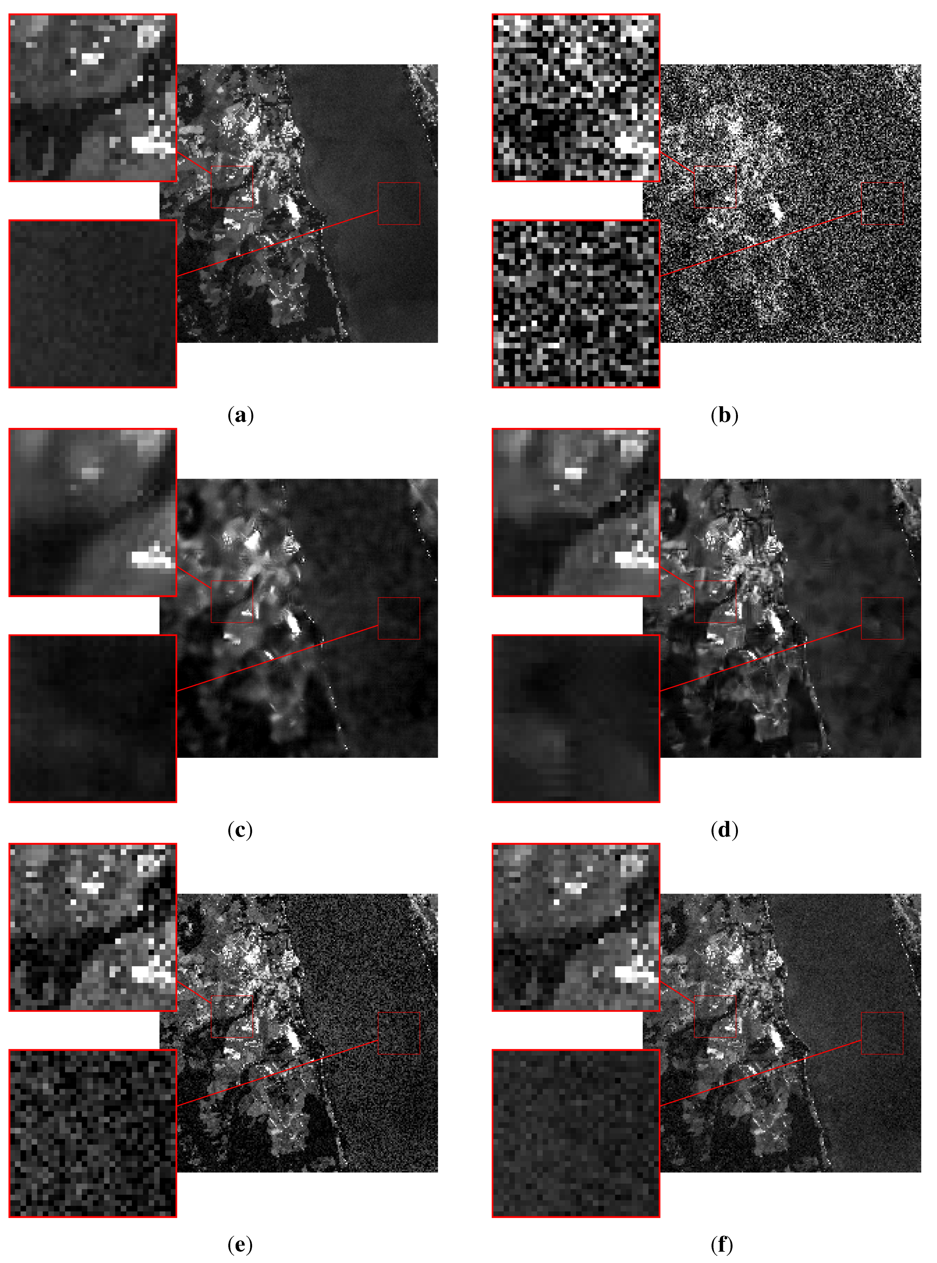
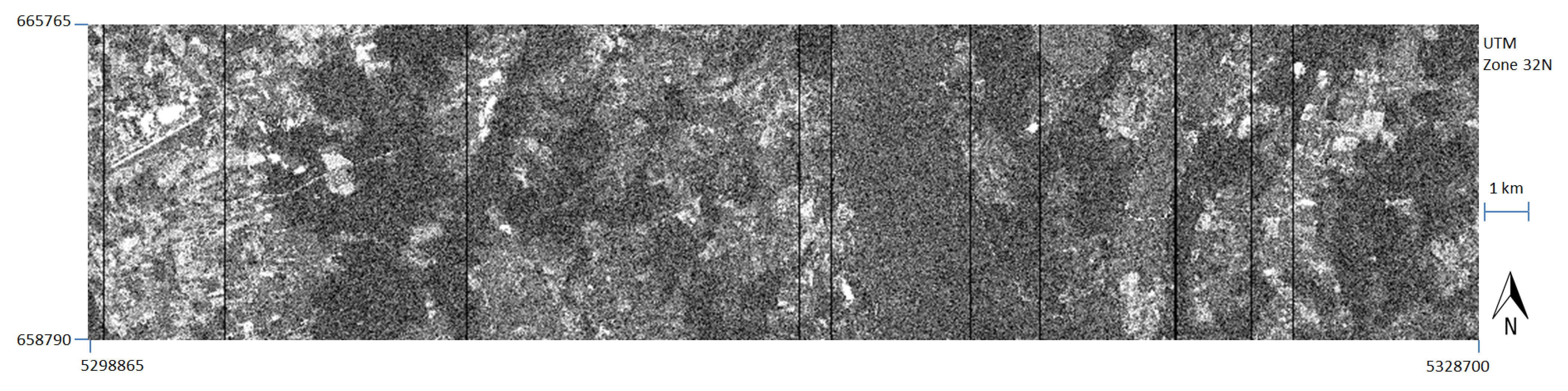
5. Denoising of Bands with a Low Signal-to-Noise Ratio

The EnMAP Alpine Foreland dataset, of size $1000\times 1000$ pixels, which has been simulated from applying water, vegetation and soil physical models to Landsat images acquired over the area around Lake Starnberg, Germany, is analyzed (for more information on the simulated dataset, see [16]). A Gaussian noise with zero mean has been added to the image in order to have an SNR equal to the worst case among the ones reported in Figure 1, of which Band 1 at 423 nm is depicted in Figure 3 and selected for the following experiments. This type of study is not simple, as all spectral bands are characterized by a low SNR (the highest one is 204 for the band centered at 479 nm), unlike traditional hyperspectral datasets in which the SNR drastically increases whenever atmospheric absorption effects become less important. The band at 423 nm is chosen as it exhibits the lowest SNR in the blue spectral range and because it contains important information, especially for water applications [17]. Furthermore, it is assumed that traditional 3D reconstruction algorithms are not very effective in this case, as only partial neighborhoods are available to model the data.

Figure 3. Band 1 from the synthetic EnMAP Alpine Foreland dataset of size $1000\times 1000$, corrupted according the worst among the predicted SNR performances in Figure 1. For the area in the red and green squares, the details are reported in Figure 4 and Figure 5.

Figure 3. Band 1 from the synthetic EnMAP Alpine Foreland dataset of size $1000\times 1000$, corrupted according the worst among the predicted SNR performances in Figure 1. For the area in the red and green squares, the details are reported in Figure 4 and Figure 5.

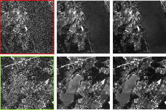
Figure 4. Denoising results on the area represented by the red square in Figure 3. The magnification of selected areas is a factor of four . (a) Original; (b) corrupted; (c) NLM; (d) BM4D; (e) unmixing-based denoising (UBD); (f) sparse UBD (SUBD).

Figure 4. Denoising results on the area represented by the red square in Figure 3. The magnification of selected areas is a factor of four . (a) Original; (b) corrupted; (c) NLM; (d) BM4D; (e) unmixing-based denoising (UBD); (f) sparse UBD (SUBD).

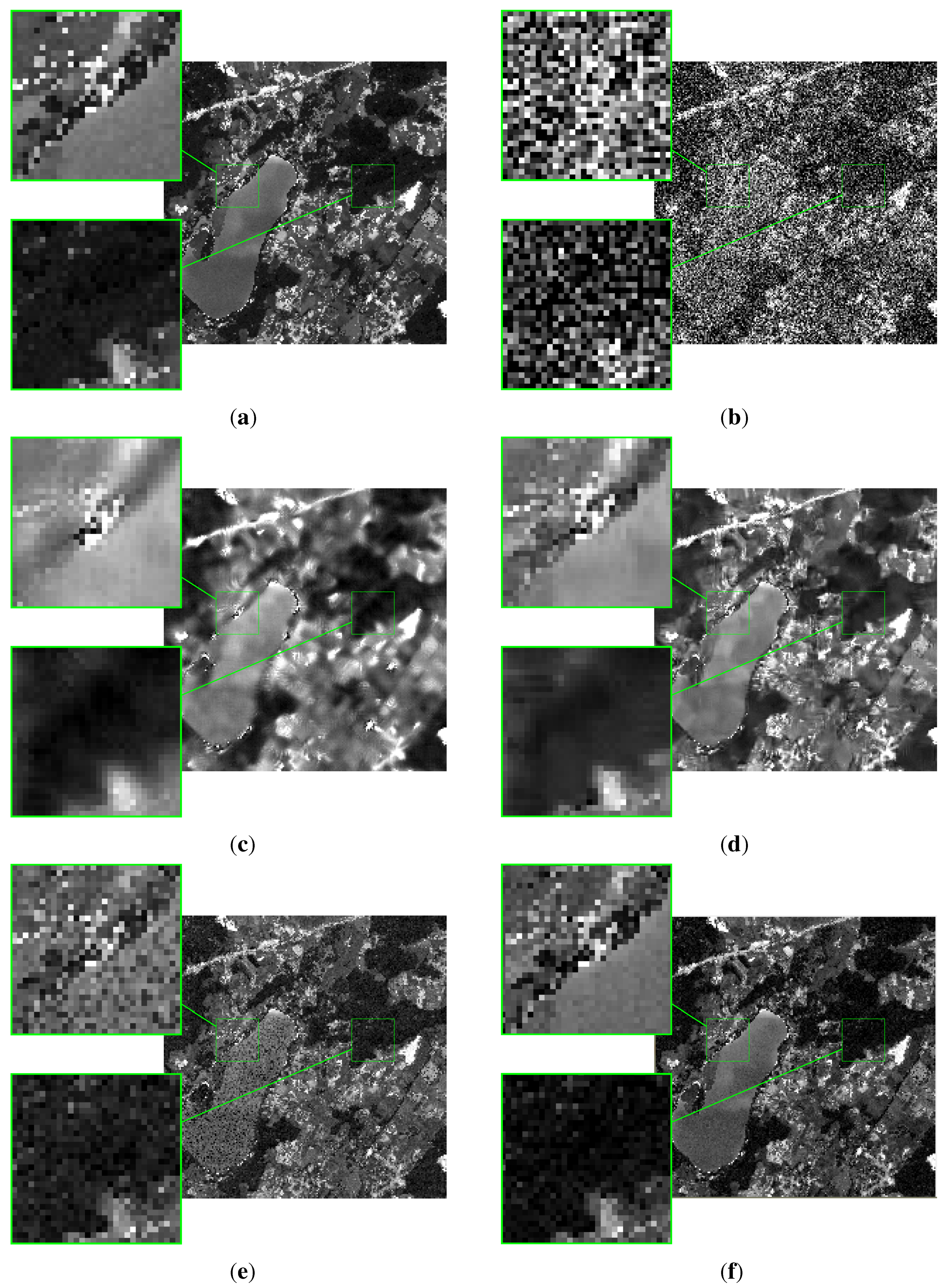
Figure 5. Denoising results on the area represented by the green square in Figure 3. The magnification of selected areas is a factor of four. (a) Original; (b) corrupted; (c) NLM; (d) BM4D; (e) UBD; (f) SUBD.

Figure 5. Denoising results on the area represented by the green square in Figure 3. The magnification of selected areas is a factor of four. (a) Original; (b) corrupted; (c) NLM; (d) BM4D; (e) UBD; (f) SUBD.

Figure 6. Sensitivity of SUBD to input parameters: (a–c) performance increase as a function of the employed dictionary size; (d) normalized root mean squared error (NRMSE) for 50 runs with different randomly-extracted dictionaries; (e–g) performance across all spectral bands applying SUBD without spectral weights (absorption bands removed in (e) due to their abnormal values; (h) sensitivity to the regularization parameter δ.

Figure 6. Sensitivity of SUBD to input parameters: (a–c) performance increase as a function of the employed dictionary size; (d) normalized root mean squared error (NRMSE) for 50 runs with different randomly-extracted dictionaries; (e–g) performance across all spectral bands applying SUBD without spectral weights (absorption bands removed in (e) due to their abnormal values; (h) sensitivity to the regularization parameter δ.

In the first step, the image is spatially smoothed with a Gaussian function with a different variance ${\sigma }_i^2$ for each band i empirically set as a function of the SNR as follows:

$${\sigma }_i^2=\frac{2}{log\left({\text{SNR}}_i\right)}$$

(5)

Afterwards, 0.3% of the image elements are randomly selected from the filtered image to initialize the overcomplete spectral library with reduced noise contributions. The denoising is then carried out on the original image as described in Equation (4), with the spectral bands weighted according to their correlation with the band of interest.

Results on denoising of two image subsets localized by the squares in Figure 3 are presented in Figure 4 and Figure 5. Even though not all of the noise is removed, it can be appreciated how the local spectral information remains unaltered with respect to the noise-free simulated dataset, as no over-smoothing of the images or morphological filters are employed by the proposed algorithm.

Figure 6a–c reports the different performances when varying the dictionary size. Some fluctuations are due to the random selections of the pixels collected in the dictionaries, but the general trend is an improvement when larger dictionaries are extracted. A set of 50 runs with different random dictionaries of 3000 elements has been performed. The results are reported in Figure 6d showing the differences to be limited, with a normalized root mean squared error (NRMSE) mostly in the range 1.8% to 1.9%, which outperforms in most cases the other denoising algorithms analyzed in this section.

Quantitative quality parameters and comparisons with alternative methods are reported in Table 1 as follows. The performance of SUBD is averaged over 50 runs with the same number of randomly-extracted dictionaries. Results are reported with and without weighting of the spectral bands in the reconstruction step and for applying traditional UBD after an automatic endmember extraction step. This is carried out by estimating the dimensionality of the dataset through hyperspectral signal subspace identification by minimum error (HySime) [18] and selecting the endmembers with Vertex Components Analysis (VCA) [19]. Comparisons are reported with the following methods: minimum noise fraction (MNF) with manual selection of the best number of components, Wiener filtering, 3D non-local means denoising [20], the BM4D volumetric denoising filter [21], Total Variation denoising [22], and a simple Gaussian filter with variance computed as in Equation (5). The figures of merit are NRMSE, expressed as a percentage (best value: 0%), structural similarity (SSIM) [23] (best value: one) and SNR (best value: ∞). Even though there is no clear 3D adaptation of SSIM for hyperspectral images (see [24]), in our experiments only a single band is taken into account, making this assessment of particular interest. The results obtained from the proposed method are consistent throughout the 50 random runs, with standard deviations ${\sigma }_{NRMSE}=0.0437$, ${\sigma }_{SSIM}=0.061$ and ${\sigma }_{SNR}=102$. The known distortions of the noisy band are also reported for reference. The second-best method in terms of NRMSE and SNR (but not of SSIM) is BM4D. However, it will be shown in the next section that this technique is not suited for images exhibiting a relevant number of missing or anomalous values. Furthermore, MNF achieves good results, as the dimensionality of the dataset derived from a multispectral image is inherently small and the noise level is constant across all of the bands. The work in [2] discusses the limits of MNF when dealing with real datasets with different noise levels in each band and higher real dimensionality; furthermore, the number of MNF components to be kept in the back rotation is hard to estimate [25]. The three-dimensional NLM filter is characterized by a low NRMSE, but from Figure 4 and Figure 5 it is clear how it destroys local information, even though edges are preserved.

Table 1. Comparison of average NRMSE, SSIM and SNR values for the denoising of the band reported in Figure 3. The values for the proposed method are averaged over 50 runs with random dictionary extraction.

	Alpine Foreland Dataset
	NRMSE (%)	SSIM	SNR
Noisy band at 423 nm	6.82	0.278	166
SUBD	1.87	0.696	2217
UBD	2.83	0.619	966
SUBD no weights	2.10	0.682	1755
MNF (best result)	2.13	0.609	1713
Wiener (best result)	3.42	0.395	662
BM4D [21]	1.98	0.592	1980
3D non-local means	2.12	0.517	1725
Total variation	2.96	0.417	885
Gaussian filter	3.87	0.383	528

Table 1. Comparison of average NRMSE, SSIM and SNR values for the denoising of the band reported in Figure 3. The values for the proposed method are averaged over 50 runs with random dictionary extraction.

	Alpine Foreland Dataset
	NRMSE (%)	SSIM	SNR
Noisy band at 423 nm	6.82	0.278	166
SUBD	1.87	0.696	2217
UBD	2.83	0.619	966
SUBD no weights	2.10	0.682	1755
MNF (best result)	2.13	0.609	1713
Wiener (best result)	3.42	0.395	662
BM4D [21]	1.98	0.592	1980
3D non-local means	2.12	0.517	1725
Total variation	2.96	0.417	885
Gaussian filter	3.87	0.383	528

The proposed method was originally designed to restore specific bands affected by noise in a given EnMAP image. Nevertheless, results applied to the full dataset without applying the weights as in Equation (3) yield good results, as summarized in Figure 6e–g. The average per-band values for NRMSE, SSIM and SNR in this case are 2.34, 0.88 and 972, respectively (21 water absorption bands as depicted in Figure 6e are considered as outliers and not included in this computation).

The setting of the regularization parameters is a known problem in sparse regression and sparse spectral unmixing [4,5,6]. However, the sum of the coefficients can be expected to be at most $\sum \left|x\right|=1$, as this is often assumed in spectral unmixing whenever the spectral library is extracted from the image itself [26]. This assumption has been assessed numerically and is reported in Figure 6h, where the performance stabilizes from $\delta =1$. As setting a larger δ does not reduce the performance but increases the execution time of the algorithm, this has been set to one for all experiments.

SUBD has been tested on the band reported in Figure 3 with no change in settings in the other two scenarios related to the expected and best SNR values as depicted in Figure 1. Results are reported in Table 2 along with the already described worst case performance for comparison.

Table 2. Comparison of SUBD performance for denoising the spectral band in Figure 3 that was corrupted at different levels of SNR (see Figure 1).

Noise Level (SNR)	SNR	NRMSE (%)	SSIM
Worst Case (166)	2217	1.87	0.696
Expected Performance (303)	3213	1.55	0.750
Best Case (535)	4914	1.22	0.800

Table 2. Comparison of SUBD performance for denoising the spectral band in Figure 3 that was corrupted at different levels of SNR (see Figure 1).

Noise Level (SNR)	SNR	NRMSE (%)	SSIM
Worst Case (166)	2217	1.87	0.696
Expected Performance (303)	3213	1.55	0.750
Best Case (535)	4914	1.22	0.800

The method is also fast in terms of running time, taking 70.47 s on a standard laptop machine with 8 GB RAM and an Intel(R) Core(TM) i5-2520M 2.50-GHz processor to denoise the one million pixels with 224 spectral bands.

6. Dead Pixel Inpainting

The term “inpainting” is centuries older than the advent of digital images, as it is used to represent the act of skilled artists of filling in damaged areas inside paintings in a way that would be non-detectable for an observer. In the image processing community, this term indicates the restoration of missing/corrupted pixels in a digital image by observing the values of their uncorrupted neighbors [27]. Inpainting techniques were soon adapted to 3D data, and in recent years, specialized algorithms have been defined for multi- and hyper-spectral data [28,29,30,31]. The problem of destriping images affected by drop-out artifacts is closely related [30], as missing values need to be restored seamlessly and could be tackled in the same way.

The coupling of UBD with sparse reconstruction allows proposing a new way to tackle this problem by exploiting the full spectral information conveyed by a corrupted image element rather than its spatial neighbors. This may be well suited for areas in which the values of neighboring pixels are not reliable due to the presence of image artifacts or noise, such as the low SNR scenario described in Section 5.

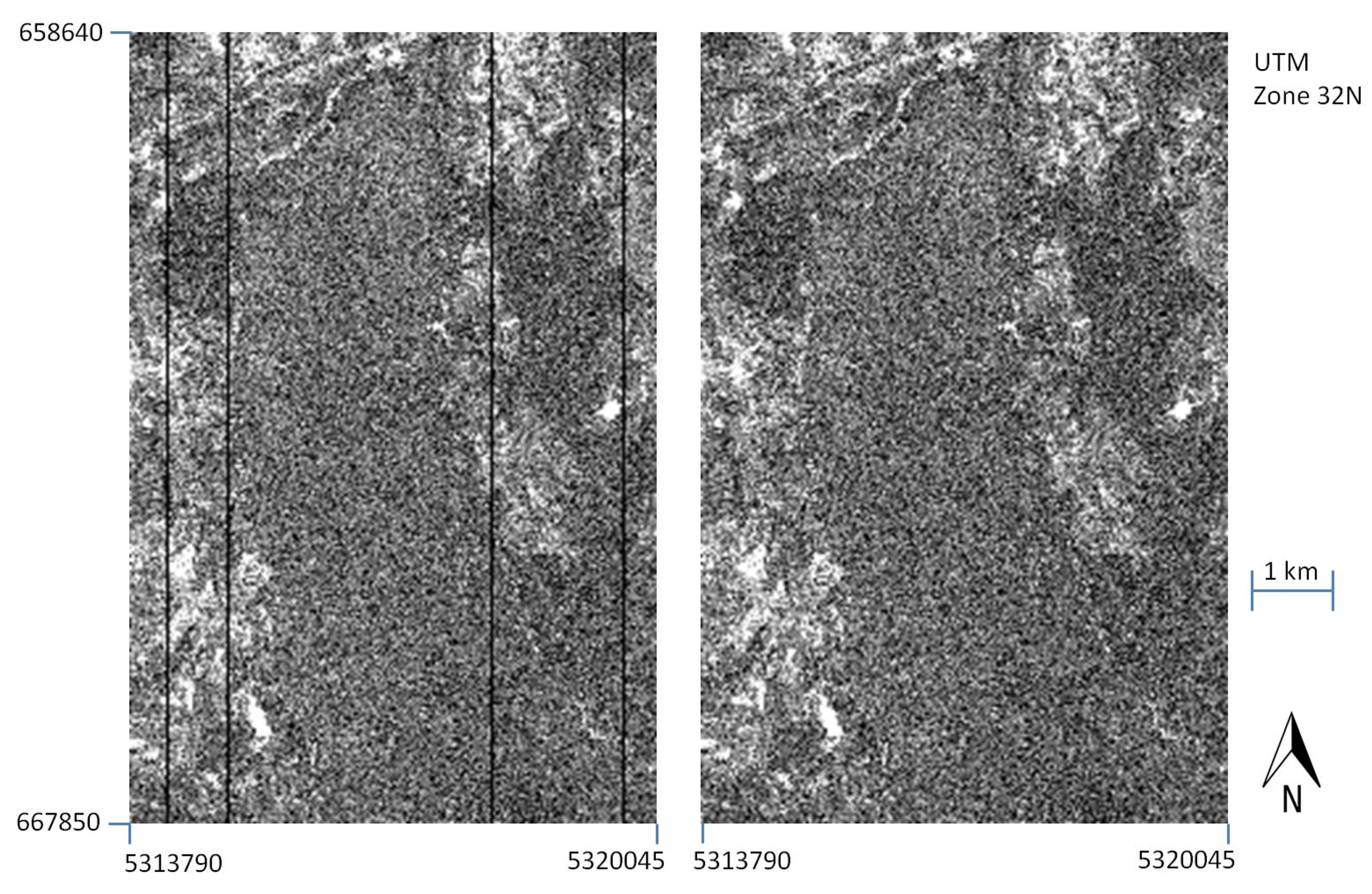
For this experiment, the simulated data are degraded as much as possible. This is achieved by introducing a high amount of dead pixels into the image with the lowest SNR, which was used in the experiments reported in Section 5. The specification of the FPA allows for up to 1% of the detector elements to be defective at end-of-life for the EnMAP mission, which is five years after launch. This serves as a worst case assumption for the simulation of a dead pixel mask for the VNIR and SWIR FPAs. Defective pixel locations on the FPA are generated randomly and transferred to the simulated EnMAP image, resulting in black columns in each of the channels of the hyperspectral image. On average, 10 black columns in each channel are differently distributed for each spectral band; a subset of Figure 3 was additionally corrupted in the described way and is reported in Figure 7.

Figure 7. Subset from Band 1 of the synthetic EnMAP Alpine Foreland dataset corrupted by 1% dead pixels appearing as black vertical lines.

Figure 7. Subset from Band 1 of the synthetic EnMAP Alpine Foreland dataset corrupted by 1% dead pixels appearing as black vertical lines.

The drop-out artifact correction results in terms of the RMSE between the original, noise-free pixels and the reconstructed ones are reported in Table 3. A comparison with three methods for the inpainting of 3D data was performed. Partial differential equation (PDE) discretization is a standard reference in this field [27], adapted to the 3D case using the code available at [32]. The second inpainting method is based on the substitution of discrete cosine transform (DCT) coefficients [33] and has been applied to remotely-sensed data in [29]. Finally, the recently proposed L0 Total Variation (L0TV) is an effective method for image restoration based on total variation, which outperforms state-of-the-art inpainting algorithms [34]. Additionally, results from BM4D, which yields a good performance in Table 1, have been computed for completeness. RMSE values are also reported for simple spatial and spectral interpolations, for which neighborhoods of different sizes have been tested (the best results are reported) and for the original values of the noisy dataset. The advantage of SUBD being able to exploit the full spectral information allows performing the inpainting with the smallest reconstruction error, corresponding to an RMSE of 2.43. It is also clear how robustly the method operates on noisy data, yielding a denoised reconstruction for missing values (for example, see Figure 8). On the other hand, it is clear that BM4D is not suited for the inpainting problem, as it treats the missing data as edges in the image, leaving them mostly unaltered. The affected pixels are correctly recognized by L0TV and reconstructed with a low overall error, but with higher distortion with respect to SUBD’s results.

Figure 8. Detail of the image partially depicted in Figure 7 (left) and the results of the inpainting algorithm based on UBD with sparse reconstruction (right).

Figure 8. Detail of the image partially depicted in Figure 7 (left) and the results of the inpainting algorithm based on UBD with sparse reconstruction (right).

The running time of the inpainting experiment was less than 10 s on the machine described for previous experiments in Section 5, as the algorithm operates pixel-wise and must be applied only to the corrupted image element, according to the available dead pixel mask.

Table 3. Comparison of average RMSE values for the dead pixel inpainting experiment applied to the image partially depicted in Figure 7.

Method	Average RMSE
Original noisy image	60.79
SUBD	2.43
Spatial interpolation	5.36
Spectral interpolation	9.30
PDE [32]	4.43
DCT [33]	7.95
L0TV [34]	3.07
BM4D [21]	60.09

Table 3. Comparison of average RMSE values for the dead pixel inpainting experiment applied to the image partially depicted in Figure 7.

Method	Average RMSE
Original noisy image	60.79
SUBD	2.43
Spatial interpolation	5.36
Spectral interpolation	9.30
PDE [32]	4.43
DCT [33]	7.95
L0TV [34]	3.07
BM4D [21]	60.09

7. Conclusions

In this paper, SUBD, a new denoising technique based on sparse reconstruction, is tested on simulated EnMAP data. The algorithm improves on the idea of UBD by increasing its automation degree and by tuning the contribution of each spectral band to the final result. The first results are encouraging, as they outperform some standard techniques, i.e., a higher SNR of 237, a higher SSIM of 0.077 and an NRMSE of 0.11% from the second-best method considering these measures. This shows the effectiveness of the proposed method at correcting EnMAP images acquired under unfavorable illumination conditions or at higher off-nadir looking angles. Furthermore, the operational fully-automatic on-ground processing, which delivers standardized products to the international user community, introduces at most 1% dead or bad pixels [11]. The proposed method is successfully tested on destriping and restoration of corrupted data, which have a non-negligible impact for practical applications. In this case, the advantage of the method of operating pixel-wise allows a fast processing restricted to the image elements to be inpainted, providing 0.64% better RMSE than the second-best method.

In the future, while waiting to test the proposed and other algorithms on real EnMAP data, further experiments will be carried out on simulated datasets derived from hyperspectral airborne data or acquired by satellites with comparable spatial and spectral resolution, such as Hyperion (although with much different SNR values). For the next experiments, a smart initialization step will be implemented to extract the reference overcomplete spectral library to be used in the sparse unmixing step. Instead of randomly selecting the spectra from the image, an endmember extraction algorithm can be used to provide a meaningful set of spectra to initialize the library. To reduce the impact of noise, algorithms for the extraction of endmember bundles [35] can be taken into account, which merge similar image elements. Subsequently, representative pixels can be located on the convex hull spanning the space of the high-dimensional data or selected on the basis of their Pixel Purity Index (PPI) [36].