1. Introduction
A recent spark of natural disasters around the world, including in Australia and New Zealand, for example the bushfire in Victoria, the flood in Queensland and the earthquake in Christchurch, has made it imperative to investigate automatic systems, which not only forecast the risk of disasters, but also help with minimising losses, such as human lives and properties, during the catastrophe and a quick recovery, including resettlement of the local communities, after the incident. These days, bushfires constitute a major natural and socioeconomic hazard, costing Australia in excess of $80 million per year and affecting around three million hectares of land in southern Australia alone [
1]. In an average year, 29 million hectares of Australia are burnt by bushfires. Government agencies in Australia and New Zealand spend hundreds of millions of dollars annually on the management of bushfires.
However, any disaster management procedure in a remote area will be ineffective when the local and state governments do not have an updated digital building map or there is a large number of informal settlements in remote and forest areas. In fact, many local and state governments in remote areas do not have a digital version of the topographic database that includes vegetation, roads and buildings. Moreover, there are a significant number of informal buildings or extensions to the already planned buildings in Australia. This informal development may decrease the state and local government revenue, may pose a serious social and economic impact on the owners, the national economy and the real estate industry or, when developed at a large scale, may have negative environmental effects [
2]. According to the Royal Australian Institute of Architects’ survey on illegal buildings, 25 percent of property buyers could get caught with an expensive renovation bill if they did not undertake a proper pre-inspection of the property [
3].
Although the state and local governments apply high penalties to owners in cases where informal constructions are detected, this alone cannot solve the problem. From a technical point of view, one common reason for the administration’s inefficiency to control unplanned development is the difficulty of locating, quickly and in time, the construction of informal buildings in a cost-effective way and stopping the construction as its beginning or applying a penalty within a short time of its completion. Classic administrative control procedures have proven inefficient, especially when public administration suffers from a lack of employees, bureaucracy and increased responsibilities. It is difficult to place inspectors in each area to stop illegal construction work, thus encouraging corruption [
2].
Recently, geographic information systems (GIS) have significantly simplified the quantification of the spatial distribution and risk levels of the elements that contribute to “bushfire risk” [
1]. In this context, a digital building map can be useful, for example in decision making, for several government and land agencies. In the case that some manual field work is necessary, then the cost of contracts can be estimated using the up-to-date map. In order to monitor the performance of the cartography agencies, the government’s quality assurance team can inspect the field to note the contradictions. The automatic change detection could even replace the field work completely, and the government can plan and monitor the urban growth, which in turn leads to significant financial savings. Moreover, an updated topographic map along with the required building and road information can be used for a multitude of purposes, including urban planning, identification of informal settlements, telecommunication planning and analysis of noise and air pollution.
However, the manual creation and update of a digital building database is time consuming and expensive. There is an increased need for map revision, without large increases in cost, in order to keep the mapping current, especially in those areas that are subject to dynamic change due to new construction and reconstruction of urban features, such as buildings and roads. Thus, automation in building detection and change detection is a key issue in the updating of building information in a topographic database. The availability of high resolution aerial imagery and LiDAR (light detection and ranging) point cloud data has facilitated the increased automation within the updating process. This paper concentrates on the automatic building change detection and semiautomatic generation and update of the building database.
Automatic building change detection from remote sensing data mainly falls into two categories [
4]. Firstly, in the direct approach, data acquired from one type of sensor on two different dates are directly compared to detect changes. Secondly, in the indirect approach, the building information is first detected from a new dataset and then compared to that in the existing map. For instance, while Murakami
et al. [
5] detected building changes by simply subtracting DSMs (digital surface models) collected on different dates, Vosselman
et al. [
6] first segmented the normalised DSM in order to detect buildings and then compared them to buildings in the map.
In the indirect approach, the presence of an existing building database is a prerequisite in order to be able to detect building changes from the newly-available data of an area. However, in many countries, such a database does not exist. The creation of a building database from high resolution aerial imagery, for instance through monoscopic image measurement using a proprietary software, such as Barista [
7], is expensive, as it takes considerable time from a human operator. Moreover, in the absence of a high resolution true orthophoto, such a manually-created database will have poor accuracy.
This paper presents a semiautomatic technique to create a new building database from LiDAR point cloud data. Buildings are first extracted using an automatic and high-performance building extraction technique. Since the result may not be 100% correct, some manual work is still required while creating the database. A graphical user interface (GUI) has been developed to facilitate a human operator to quickly decide about the extracted buildings, edit them if necessary, delete the false detections and add the missing buildings, if any. Interested industries and government organisations may use this database for their purposes.
In the case that there is a need for updating the old building database with the help of a newly-available dataset, the paper proposes a new building change detection technique by comparing the extracted building information from the new dataset to that in an existing building database. A connecting component analysis-based technique is proposed to remove the false changes and thereby identify actual changes. Again, since the detected changes are not 100% correct, the GUI is used to allow the user to quickly rectify the building change detection result before the map database is actually updated. The GUI can be facilitated with an orthophoto of the study area. It helps with reducing the human labour considerably when compared to the manual creation and update of the database.
Since the manual building change detection is expensive, the aim of this research is to develop a semiautomatic system that allows for periodic monitoring and detection of building changes using LiDAR point cloud data. Different types of changes get updated in the database with a low amount of manual effort. An estimation of the amount of human interaction in the proposed system compared to the totally manual system is presented. The quality of the generated building map is also estimated in order to validate the application of the proposed system. Note that the initial version of this research has been published in [
8]. In the current submission, the research has been refined and explained in detail and tested and evaluated using new, large datasets. A sensitivity analysis of some algorithmic parameters, as well as an estimation of the manual work required during the generation and update of the map database are also conducted and presented. In addition, a performance comparison between the proposed and the existing change detection methods has been discussed.
The rest of the paper is organised as follows. A brief discussion of the relevant building change detection techniques and their performance evaluation indicators is presented in
Section 2.
Section 3 presents the proposed approach of building map generation, change detection and map updating.
Section 4 discusses the evaluation strategy, the study area and experimental results. Finally,
Section 5 concludes the paper.
2. Related Work
For building change detection, there are three categories of techniques, based on the input data: image only [
2,
9,
10], LiDAR only [
6] and the combination of image and LiDAR [
11]. The comprehensive comparative study of Champion
et al. [
12] on building change detection techniques showed that LiDAR-based techniques offer high economic effectiveness. Moreover, change detection from aerial imagery alone is less effective due to shadows from skyscrapers and dense vegetation, diverse and ill-defined spectral information and perspective projection of buildings [
13]. Thus, this paper primarily concentrates on techniques that use at least LiDAR data. The relevant performance evaluation indicators for building change detection are also reviewed.
2.1. Change Detection Techniques
In regard to direct change detection approach, Zong
et al. [
14] proposed a technique by fusing high-resolution aerial imagery with LiDAR data through a hierarchical machine learning framework. After initial change detection, a post-processing step based on homogeneity and shadow information from the aerial imagery, along with size and shape information of buildings, was applied to refine the detected changes. Promising results were obtained in eight small test areas, but its performance was limited by the training dataset. Murakami
et al. [
5] subtracted one of the LiDAR DSMs from three others acquired on four different dates. The difference images were then rectified using a straightforward shrinking and expansion filter that reduced the commission errors. The parameter of the filter was set based on prior knowledge about the horizontal error in the input LiDAR data. The authors reported no omission error for the test scene, but they did not provide any statistics on the other types of measurements.
Vu
et al. [
13] applied thresholds to the height histogram generated from the difference DSM image. A point density threshold was also employed in order to remove artefacts. However, this technique divided the changes only into new and demolished classes and, thus, could not identify the changed building classes,
i.e., extended and demolished building-parts. Moreover, it was unable to discriminate between buildings and trees. Choi
et al. [
15] first obtained the changed patches (ground, vegetation and buildings) by subtracting two DSMs generated from the LiDAR point clouds from two dates. Then, LiDAR points within the obtained patches of each date were segmented into planes using a region growing method. Features, such as area, height and roughness, were applied to the planes of each date in order to classify them into ground, vegetation and building classes. Finally, the plane classes from two dates were compared based on their normal vectors, roughness and height to classify the changes to/from ground, vegetation and buildings. However, this approach failed to detect different types of building changes, for instance new and demolished buildings.
Among the indirect approaches to building change detection, Matikainen
et al. [
16] used a set of thresholds to determine building changes and showed that the change detection step is directly affected by the preceding building detection step, particularly when buildings have been missed due to low height and tree coverage. Thus, a set of correction rules based on the existing building map was proposed, and the method was tested on a large area. High accuracy was achieved (completeness and correctness were around 85%) for buildings larger than 60 m
2; however, the method failed to detect changes for small buildings.
Grigillo
et al. [
4] used the exclusive-OR operator between the existing building map and the newly-detected buildings to obtain a mask of building change. A set of overlap thresholds (similar to [
16]) to identify demolished, new, extended and discovered old (unchanged) buildings was then applied, and per-building completeness and correctness of 93.5% and 78.4%, respectively, were achieved. Rottensteiner [
11] compared two labelled images (from the existing map and automatic building detection) to decide building changes (confirmed, changed, new and demolished). Although, high per-pixel completeness and correctness measures (95% and 97.9%) were obtained, the method missed small structures. The method by Vosselman
et al. [
6] ruled out the buildings not visible from the roadside (e.g., buildings in the back yard) and also produced some mapping errors. Olsen and Knudsen [
17] removed the non-ground objects smaller than 25 m
2 during classification of buildings and vegetation. Thus, it was unable to detect changes caused by small buildings. Moreover, the detail of the building change detection procedure was missing from the published account [
17].
Malpica and Alonso [
18] applied support vector machines (SVM) to detect changes from satellite imagery and LiDAR data. Trinder and Salah [
19] combined four change detection techniques based on machine learning algorithms (SVM, minimum noise fraction,
etc.) to aerial imagery and LiDAR data and employed simple majority voting for the final change detection. An improved detection accuracy, as well as a low segmentation error were observed with the combined approach when compared to the individual approaches alone. The success of the techniques that employ the supervised learning algorithms are limited as they may not work on a given new dataset unless a new set of training samples is provided. Moreover, the parameters of the involved learning algorithm may require re-tuning for a new test dataset.
There are also building detection and change detection techniques using point cloud data generated through dense image matching. For example, Xiao
et al. [
20] defined building hypotheses using the facade generated using the height information from the dense image matching technique. The initial buildings were then verified and refined employing the image-based point cloud data. Experimental results on buildings of at least 25 m
2 in area showed that this method was able to achieve a completeness of 85% for regular and 70% for irregular residential buildings. Nebiker
et al. [
10] generated image-based dense DSM from historical aerial imagery and then applied an object-based image analysis for building detection. For densely-matched DSM, this technique achieved a building detection completeness of more than 90% for buildings of at least 25 m
2 in area. Vetrivel
et al. [
21] developed a methodology to delineate buildings from an image-derived point cloud and classified the present gaps to identify damage in buildings. The gaps due to damage were identified by analysing the surface radiometric characteristics around the gaps. A gap due to architectural design is more homogeneous in nature and possesses a uniform radiometric distribution, whereas a damage region tends to show irregular radiometric distribution. This technique detected 96% of the buildings from a point cloud generated using airborne oblique images. The learning model based on Gabor features with random forests identified 95% of the damaged regions. Qin [
22] and Tian
et al. [
23] employed the height difference information from DSMs of two different dates for building change detection. An evaluation on large buildings (>200 m
2) showed an overall correctness of 87% by the technique in [
22]. More image-based building (change/damage) detection techniques can be found in comprehensive reviews in [
10,
21,
24].
In 2009, under a project of the European Spatial Data Research organisation, Champion
et al. [
12] compared four building change detection techniques and stated that only the method in [
11] had achieved a relatively acceptable result. Nevertheless, the best change detection technique in their study was still unsuccessful in the reliable detection of small buildings. Therefore, there is a significant scope for the investigation of new automatic building change detection approaches.
In general, methods following the direct change detection approach face the problem of removing vegetation changes, which is obvious if the data are captured on two different dates. Methods employing the machine learning algorithms, e.g., SVM, may not work well in a given new dataset if the appropriate training data are not provided. Methods that are based on the DSM have a significant negative impact on the change detection results [
11].
The proposed method in this paper follows the indirect approach where trees are mostly eliminated in the building detection step, so it faces less problems in the building change detection step. Moreover, raw point cloud data are used in order to avoid problems associated with the DSM. A feature-based approach has been proposed in this paper that avoids the need for a training dataset, which is necessary for methods involving machine learning algorithms.
2.2. Evaluation of Change Detection
Many of the published change detection techniques [
5,
6,
13,
15,
25] did not present any objective evaluation results; rather, visual results were presented from one or two test datasets. The use of a small number of test datasets might be due to the unavailability of the datasets of the same test area from two different dates, where some changes could be present at a given time interval.
For the evaluation of building change detection performance, the manually-created ground truth information of the building changes is compared to that detected by the obtained change detection results. The creation of the reference/ground truth data can be obtained through human visual interpretation and digitisation using two datasets (from two dates) of a test area: an old building map and a new aerial image or two aerial images from two dates. Different pixel- or area-based, as well as object-based performance indicators have been used in the existing work.
In pixel-based evaluation, Trinder and Salah [
19] used detection accuracy and area omission and commission errors. Rottensteiner [
11] used the completeness, correctness and quality of the detected changes. In addition to completeness and correctness, Zong
et al. [
14] employed overall accuracy and false alarm rate.
In object-based evaluation, Olsen and Knudsen [
17] tabulated the change detection results using the numbers of different types of changes [
17]. Grigillo
et al. [
4] measured completeness and correctness for all of the changes together. Champion
et al. [
9] presented completeness and correctness measurements both in object- and pixel-based evaluations. Matikainen
et al. [
16] showed the change detection result by the numbers of different types of changes, as well as completeness and correctness.
The aim of a building change detection technique is to guide the human user’s attention to the changed buildings, so that the unchanged buildings are not inspected at all. Ideally, both completeness and correctness performance indicators of a change detection method should be 100%. While a high completeness value increases the quality of the updated database, a high correctness value reduces the amount of the required human inspection. However, in practice, the completeness value may be compromised if changes relevant to (small) buildings/building-parts are not automatically detected. Such omission errors will require human intervention, which may cause manual inspection of the whole test area in the worst case, even for identification of a single missed change. Furthermore, the correctness value may not be maximum due to false change detections, mainly caused by detected trees and missing (small) buildings by the involved building detection technique.
The quality of building change detection result is more understandable in object-based evaluation than in pixel-based evaluation. In applications such as bushfire management and the identification of informal settlements, the per-building (actually per change when more than one change may be present in a single building) is more meaningful than the pixel- or area-based evaluation. In fact, the effectiveness of a change detection technique is limited by the number of changes, not by the area covered by the changes. Consequently, in this paper, the building change detection result has been expressed using the number of true and false changes against the reference change information. In addition, object-based completeness and correctness are also provided.
3. Proposed Approach
Figure 1 shows the flow diagram of the proposed approach. It has two main steps: (i) creation of the building database and (ii) building change detection and update of the database.
In order to create a building database, buildings are first extracted from an old dataset (from an early date) of a test area. A high-performance automatic building detection technique [
26] has been implemented for this purpose. The extracted buildings are two-dimensional building footprints, where each footprint is a polygon showing the boundary of each building. The height around the building boundary is also available from LiDAR point cloud data. Then, the extracted buildings are overlaid on the orthophoto and checked by a human operator via the developed GUI. The main task of the operator includes removal of false detections, mainly trees, splitting and merging of footprints due to under- and over-segmentation errors and adding any missing buildings. If any extracted building footprint includes nearby vegetation, then the operator can edit the boundary as necessary. The editing tool can also be used to include the required level of detail in the building map by editing small details around the building boundary. The output from the GUI constitutes the building map or database.
Figure 1.
Flow diagram for the proposed creation and update of the building database.
Figure 1.
Flow diagram for the proposed creation and update of the building database.
When time comes to update the building database, a new dataset is provided to the automatic building detection technique. The newly-extracted building footprints are compared to those in the existing building database. A connecting component analysis-based automatic change detection technique has been proposed to remove the false changes and thereby identify the actual changes in buildings. The changes are classified as new, demolished and changed. While the new class indicates the buildings that are newly built, the demolished class contains the buildings that are totally demolished. The changed class can be due to the extension of an existing building (subclass: new-part) and destruction of a part of an existing building (subclass: demolished-part). If an existing building is completely demolished and a new building is rebuilt in the same place, such a change can be detected by means of one or more new-part and/or demolished-part. The unchanged buildings may also be retained in case the replacement of an existing building footprint with a new building footprint increases the quality of the database. The detected changes are highlighted over the old (from the database) and new building footprints (overlaid on a new orthophoto) in the GUI. The human operator decides about the highlighted changes and the replacement of any existing footprints with the new footprints.
The purpose of the GUI is to allow for human interaction at a minimum level. While the true changes are accepted by simply clicking on them, the false changes are just ignored. The decision of the replacement of an existing footprint with a new version can be simply indicated by a mouse click within the two footprints. In the following sections, all of the steps in the workflow are presented.
3.1. Automatic Building Extraction
The high-performance automatic building extraction technique by Awrangjeb
et al. [
26] has been implemented. This technique first divides the input LiDAR point cloud data into ground and non-ground points by using a height threshold with respect to the ground height. The non-ground points, representing objects above the ground, such as buildings and trees, are further processed for building extraction. Points on walls are removed from the non-ground points, which are then divided into clusters. Planar roof segments are extracted from each cluster of points using a region-growing technique. Planar segments constructed in trees are eliminated using information, such as area, orientation and unused LiDAR points within the plane boundary. Points on the neighbouring planar segments are accumulated to form individual building regions. An algorithm is employed to regularise the building boundary [
26]. Lines along the boundary are first extracted, and then, the short lines are adjusted with respect to the long lines through maintaining the parallel and perpendicular property among the lines. The final output from the method consists of individual building footprints.
Figure 2 shows an example of building detection from a sample dataset. The input point cloud data in
Figure 2a are shown in colour with high (roof) points in red and low (ground) points in blue.
Figure 2.
Building detection from point cloud data: (a) input point cloud overlaid on an aerial image; (b) non-ground point cloud data (3D view), where point clusters are shown in different colours; (c) extracted planar roof segments (3D view); (d) plane boundaries of the finally chosen planar segments; (e) building boundary; and (f) regularised building boundary. The coordinate and scales for easting (E) and northing (N) in (b) to (f) are the same as those shown in (a). The height axis in (b) and (c) is the same and shows the elevation values.
3.2. Generating the Building Map
A simple GUI (graphical user interface) has been developed to allow the user to generate a building map database from the automatically-generated building footprints. As shown in
Figure 3, the GUI shows the building outlines using cyan-coloured polygons. The GUI, which in general has the following functions, can be interacted with by a human operator to refine the footprints and to save them as a building map database. A function is executed as soon as the key “F” is pressed following the required mouse clicks for that function.
Figure 3.
A simple GUI for the generation of the building map database.
Figure 3.
A simple GUI for the generation of the building map database.
Addition: To add a missing building, the user can draw a regular polygon for the new building by clicking on building corners.
Deletion: To remove false buildings, which are usually vegetation, the user can draw a polygon around one or more false buildings to specify the region. All buildings within the specified region will be deleted.
Merge: In order to merge two extracted footprints, which are actually for one building, the user can merge them by clicking on the two close boundary segments. This function handles the over-segmentation problem during building extraction.
Split: In order to split an extracted footprint that covers two or more actual buildings, the user can click on consecutive points along which the footprint must be split. This function handles the under-segmentation problem during building extraction.
Edit: The user can rectify any other building delineations in the map. This will be helpful when a recent high-resolution orthophoto is available.
Undo: The user can undo the previous action.
Save: The updated map can be saved at any time.
In general, the GUI is capable of generating a new building map by simply using an orthophoto and/or automatically-extracted building footprints.
3.3. Proposed Building Change Detection Technique
The proposed building change detection technique is presented here with the help of
Figure 4. The technique uses two sets of building information as input: an existing building map and the automatically-detected building footprints from a new dataset (
Figure 4a,b). These input data are in the form of 2D regular polygons representing the building footprints. In order to obtain changes between the inputs, a 2D grid of cells (pixels) with a resolution of 0.5 or 1 m (e.g., resolution of the inputs) is used to simply compare the input information. Through comparison, four masks with the same resolution as the grid are generated.
Figure 4.
Change detection: (a) existing building map; (b) extracted buildings from new data; (c) mask from (a) and (b) showing old, new and existing building/parts; (d) mask for old building-parts only; (e) morphological opening of (d); (f) estimation of the length and width of a component; (g) mask for new building-parts only; (h) morphological opening of (g); (i) final change detection results. The coordinates and scales for easting (E) and northing (N) in (b) to (e) and (g) to (i) are the same as those shown in (a).
The first mask
M1, shown in
Figure 4c, is a coloured mask that shows three types of building regions. The blue regions indicate no change,
i.e., buildings exist in both inputs. The red regions indicate building regions that exist only in the existing map. The green regions indicate new building regions,
i.e., the newly-detected building outlines.
The second mask
M2, depicted in
Figure 4d, is a binary mask that contains only the old building-parts (not the whole buildings). As shown in
Figure 4g, the third mask
M3 is also a binary mask that contains only the new building-parts (again, not the whole buildings).
The fourth mask
M4 is a coloured mask that shows the final building change detection results (see
Figure 4i). Initially, the new and old (demolished) “whole building” regions are directly transferred from
M1. Then, the demolished and new building-parts are marked in the final mask after the following assessment is applied to
M2 and
M3.
There may be misalignment between the buildings from the two input data sources. As a result, there can be many unnecessary edges and thin black regions found in
M2 and
M3. These small errors in either mask increase the chance that buildings will be incorrectly classified as changed. Assuming that the minimum width of an extended or demolished building-part is 3 m [
6], a morphological opening filter with a square structural element of
Wm = 3 m is applied to
M2 and
M3 separately. As can be seen in
Figure 4e,h, the filtered masks
M2f and
M3f are now almost free of misalignment problems.
Next, a connected component analysis algorithm is applied to
M2f and
M3f separately. The algorithm returns an individual connected component along with its area (number of pixels), centroid and the orientation of the major axis of the ellipse that has the same normalized second central moments as the component’s region. Two corresponding MATLAB functions
bwconncomp and
regionprops have been applied to obtain the connected components and their properties (area, centroid, surrounding ellipse,
etc.), respectively [
27]. Small regions having areas less than the threshold
Ta are removed.
Figure 4f shows a region from
M3f in
Figure 4h, along with its centroid
C and the ellipse with its two axes. The width and length of the region can now be estimated by counting the number of black pixels along the two axes that pass through
C. If both the length and width are at least
Wm, then the region is accepted as a demolished (for
M2f) or new (extended, for
M3f) building-part. If they are not,
C moves along/across the major and/or minor axes to iteratively check if the region has the minimum required size. In
Figure 4f, a new position of
C is shown as
C′, and the two lines parallel to the two axes are shown by dashed lines.
The demolished and extended building-parts are consequently marked (using pink and yellow colours, respectively) in
M4, which is the final output of the proposed change detection technique. Although there are many under-segmentation cases from the building detection phase (
i.e., buildings are merged as seen in
Figure 4b),
Figure 4i shows that the proposed change detection technique is robust against such segmentation errors being propagated from the building detection phase. Moreover, the proposed change detection technique is almost free from omission errors (
i.e., failure to identify any real building changes), but it has some commission errors, which are mainly propagated from the building detection step, specifically when the involved building detection technique fails to eliminate vegetation completely, as shown by the yellow regions in
Figure 4i.
3.4. Updating Building Map
The GUI can now be used to update the existing building map using the automated change detection results.
Figure 5 shows the footprints from the existing building database using cyan polygons, the extracted buildings from the new dataset in red polygons and the final change result (mask
M4) using dots in different colours. Thus, the user can look at the suggested colour-coded changes overlaid on the orthophoto and decide which should be applied to the map (see the magnified snapshot in
Figure 5). The user can simply avoid a commission error by taking no action, and an actual change can be accepted by selecting one or two of the functional tools discussed earlier or their equivalent functions, as discussed below.
Figure 5.
The GUI to update the building map database.
Figure 5.
The GUI to update the building map database.
Replacement: The new input dataset is usually of high resolution compared to the old dataset. Thus, the newly-extracted footprint may be extracted with better quality. The user can simply replace an existing footprint with the corresponding new footprint by clicking any point within the two footprints.
Inclusion: Looking at a green region, which is a suggested true new building, the user can click a mouse button on the region. The corresponding newly-extracted building footprint will be included in the database. Alternatively, the user can draw a regular polygon for the new building using the addition tool discussed above.
Removal: In order to remove a true demolished building, the user just clicks on the suggested red region. Alternatively, the user can use the deletion tool to remove one or more demolished buildings at a time.
Extension: In order to merge a true new building-part (yellow region) with an existing building footprint, the user first adds the part to the map using the inclusion (or addition) tool and then merges it with an existing building using the merge tool. Alternatively, the changed building in the existing map can be directly replaced with its extended version from the building detection phase by using the replacement tool.
Shrink: In order to remove a true demolished building-part (pink region) attached to an existing building, the user clicks on the pink region, which will be removed from the corresponding building; or, the user can click on consecutive points along which the building must be split. The part that contains the pink region can be removed using the removal tool. Alternatively, the changed building in the existing map can be directly replaced with its new version from the building detection phase by using the replacement tool.
Moreover, the edit, undo and save tools discussed in
Section 3.2 are available to use during the update of the building database.
4. Performance Study
The performance study conducted to validate the performance of the proposed building database creation and update through automatic building detection and change detection is presented in detail in this section. Firstly, the study area and the involved evaluation strategy are presented. Secondly, a sensitivity analysis is presented for setting up the values for some important algorithmic parameters. Finally, the evaluation results are presented and discussed separately for building detection, change detection, building generation and updating.
4.1. Study Area
The test datasets covered the area of Eltham in Victoria, Australia. Four test scenes were available. While the terrain was hilly for all of them, the vegetation was dense to low in these scenes. LiDAR point cloud data from two different dates (2007 and 2012) were available. There were also orthophotos available for the test areas. The image resolution was 40 cm and 30 cm for two captured dates in 2007 and 2012, respectively. These orthophotos were mainly used to manually collect the reference building information. They were also used in the GUI to make decisions on the result from the automated change detection technique. Since, the orthophotos were generated from the aerial imagery, which had been captured on different dates of the years, there were some information gaps between the two data sources. For example, the LiDAR point cloud data of Scene 1 were taken on a later date than the aerial imagery in 2007. That is why we see that although there was a big building detected at the top-left side of Scene 1 from the LiDAR point cloud data, there was no building found in the orthophoto (see
Figure 6a).
Figure 6.
Automatic building detection in four scenes (overlaid on the orthophoto). The left column shows results from 2007 datasets and the right column from 2012 datasets. (a,b) Scene 1, (c,d) Scene 2, (e,f) Scene 3, and (g,h) Scene 4. The coordinates (easting (E), northing (N)) and scales shown for (a), (c), (e) and (g) are applicable to (b), (d), (f) and (h), respectively.
Table 1 shows some characteristics of the test scenes for both of the dates. The point density (number of points divided by the area) varied from four to six points/m
2 for the scenes in 2012 and from one to five points/m
2 in 2007. The amount of small buildings in Scene 1 was the highest on both of the dates, followed by Scene 2. There were many garages and garden sheds in these areas. Compared to the other three scenes, Scene 4 was a newly-built-up area where small garden sheds were rarely observed.
The number of completely new buildings in 2012 in four scenes was 22, 31, 8 and 72, respectively, and that of the extended buildings (new building-parts) was 1, 3, 7 and 6, respectively. The number of fully-demolished buildings in Scenes 1 and 4 was five and three, respectively; in the other two scenes, there were no totally-demolished buildings. There were three partly-demolished buildings (demolished building-parts) in Scene 1 only.
Table 1.
Four test datasets, each from two dates: dimensions in metres; point density in points/m2; B corners are the total number of corners in all reference buildings; B size indicates the number of buildings with 10 m2, 25 m2 and 50 m2 in area, respectively; vegetation: D = dense, M = moderate and L = low.
| Scenes | Dimension | P Density | Buildings | B Corners | B Size | Vegetation |
|---|
| 1, 2007 | 504 × 355 | 1.03 | 97 | 1169 | 4,13,23 | L |
| 1, 2012 | 503 × 354 | 5.33 | 117 | 1405 | 4,15,27 | L |
| 2, 2007 | 804 × 583 | 4.92 | 209 | 1735 | 0,7,17 | D |
| 2, 2012 | 806 × 584 | 5.73 | 241 | 2049 | 0,14,28 | D |
| 3, 2007 | 627 × 454 | 3.06 | 106 | 870 | 1,5,12 | M |
| 3, 2012 | 627 × 455 | 4.17 | 114 | 958 | 1,6,14 | D |
| 4, 2007 | 805 × 584 | 5.16 | 87 | 718 | 0,2,9 | M |
| 4, 2012 | 805 × 584 | 5.16 | 162 | 1385 | 0,3,12 | D |
4.2. Evaluation System
In order to evaluate the performance at each step of the flow diagram in
Figure 1, the result is presented in different steps: building detection (for both old and new datasets), map generation, change detection and map updating.
Firstly, for the evaluation of the building detection performance, 2D reference data were created by monoscopic image measurement using the Barista software [
7] for all of the test datasets. Three categories of evaluations (object based, pixel based and geometric) have been considered. A number of metrics are used in the evaluation of each category. While the object-based metrics (completeness, correctness, quality, detection and reference cross-lap rates) estimate the performance by counting the number of buildings, the pixel-based metrics (completeness, correctness, quality, area omission and commission errors) show the accuracy of the extracted buildings by counting the number of pixels. In addition, the geometric metric (root mean square error, RMSE) indicates the accuracy of the extracted boundaries with respect to the reference entities. The definitions and how these metrics are estimated have been adopted from [
28].
During the evaluation, the object-based, pixel-based and geometric metrics were automatically determined via the involved threshold-free performance evaluation technique [
29]. The minimum areas for small and large buildings have been set at 10 m
2 and 50 m
2, respectively. Small and medium-sized buildings are usually between 10 and 50 m
2 in size and mainly include garage and garden sheds. Large buildings are at least 50 m
2 in area and constitute main buildings, such as houses and industrial buildings. In most test datasets, there were also buildings, mainly carports and garden sheds, that were less than 10 m
2 in area. Thus, the object-based completeness, correctness and quality values will be separately shown for all, small and large buildings.
Secondly, for the estimation of change detection performance, the reference change information was manually counted by looking at the orthophotos of two dates for each test dataset. The building change has been categorised into four groups: new buildings (N), new or extended building-parts (NP), demolished buildings (Dm) and demolished building-parts (DP).
The change detection result is obtained from the proposed automatic change detection technique, and true positive (actual change) and false positive (commission error) values of the detected changes are counted when the change detection result, along with the existing map and the new orthophoto, is shown on the GUI. The false negative value (omission error, missing buildings or building-parts) is also estimated by looking at the orthophoto.
Thirdly, for the estimation of the amount of manual effort, deletion (D), addition (A), split (S) and merge (M) operations are counted. In addition, the number of edited buildings and the required number of mouse clicks are also estimated. These results are compared to the number of reference footprints (buildings) and their corners to estimate the amount of reduced workload.
Finally, the quality of the generated and updated building maps are estimated in terms of pixel-based and geometric metrics used for the estimation of the building detection performance.
4.3. Parameter Setting
The setting of values for parameters associated with the involved building detection technique was presented in [
30]. Therefore, in this current study, a discussion is provided for setting up the value of two parameters, the size of the structural element of the involved morphological opening filter
Wm and the area threshold
Ta, used in the proposed building change detection technique (
Section 3.3).
The value of
Wm is set at 3 m, which is set as the minimum building length or width by many studies [
6,
28]. This will remove many small unnecessary edges and thin black regions found in the two masks (
M2 and
M3) relevant to the new and demolished building-parts, respectively. Such small changes are usually found due to misalignment and/or resolution differences between the existing map and the new building detection results.
For
Ta, a sensitivity analysis is experimentally conducted in order to find a suitable value.
Table 2 shows the completeness and correctness values of the proposed change detection technique when the area threshold
Ta varies within the minimum areas of small and large building sizes (10 and 50 m
2, respectively) [
30]: five values, 9, 16, 25, 36 and 49 m
2, were tested.
Table 2.
Completeness and correctness of the change detection technique at different area threshold values.
Table 2.
Completeness and correctness of the change detection technique at different area threshold values.
| Changes | Completeness Cm (%) | Correctness Cr (%) |
|---|
| Area Threshold Ta (m2) |
|---|
| 9 | 16 | 25 | 36 | 49 | 9 | 16 | 25 | 36 | 49 |
| Scene 1 |
| Demolished | 100 | 100 | 100 | 100 | 100 | 31.3 | 41.7 | 55.6 | 100 | 100 |
| New | 100 | 100 | 100 | 86.4 | 86.4 | 84.6 | 95.7 | 100 | 100 | 100 |
| Demolished-parts | 100 | 100 | 100 | 100 | 100 | 5.9 | 18.8 | 18.8 | 33.3 | 42.9 |
| New-parts | 100 | 100 | 100 | 100 | 100 | 50 | 50 | 50 | 50 | 50 |
| Average | 100 | 100 | 100 | 96.6 | 96.6 | 42.9 | 51.5 | 56.1 | 70.8 | 73.2 |
| Scene 2 |
| Demolished | –a | – | – | – | – | – | – | – | – | – |
| New | 100 | 96.8 | 87.1 | 71 | 64.5 | 75.6 | 100 | 100 | 100 | 100 |
| Demolished-parts | – | – | – | – | – | – | – | – | – | – |
| New-parts | 100 | 100 | 100 | 100 | 100 | 13.6 | 13.6 | 16.7 | 23.1 | 27.2 |
| Average | 100 | 98.4 | 93.6 | 85.5 | 82.3 | 44.6 | 56.8 | 58.3 | 61.5 | 63.6 |
| Scene 3 |
| Demolished | – | – | – | – | – | – | – | – | – | – |
| New | 100 | 100 | 100 | 100 | 87.5 | 38.1 | 42.1 | 66.7 | 80 | 100 |
| Demolished-parts | – | – | – | – | – | – | – | – | – | – |
| New-parts | 100 | 100 | 100 | 100 | 71.4 | 53.9 | 53.9 | 70 | 100 | 100 |
| Average | 100 | 100 | 100 | 100 | 79.4 | 46 | 48 | 68.3 | 90 | 100 |
| Scene 4 |
| Demolished | 100 | 100 | 100 | 100 | 100 | 42.9 | 42.9 | 42.9 | 42.9 | 75 |
| New | 100 | 100 | 94.4 | 93.1 | 90.3 | 96 | 98.6 | 100 | 100 | 100 |
| Demolished-parts | – | – | – | – | – | – | – | – | – | – |
| New-parts | 100 | 100 | 100 | 100 | 100 | 66.7 | 66.7 | 66.7 | 66.7 | 85.7 |
| Average | 100 | 100 | 98.2 | 97.7 | 96.8 | 68.5 | 69.4 | 69.8 | 69.8 | 86.9 |
For Ta = 9 m2, while the completeness value is maximum in all four scenes, the correctness value is less than 50% in the first three scenes. This means a small area threshold will allow one to detect all small changes, but at the same time, it will generate many false alarms. For a medium threshold between 16 and 36 m2, while the completeness value is mostly above 90%, the correctness varies between 50% and 70%. This indicates that some of the small but true changes will be missed when a medium value for Ta is set. If small changes do not need to be considered, a large value of Ta will increase the correctness value, mostly above 79%, while keeping the completeness value at about 80% or above.
It is an objective of an automatic change detection technique to avoid omission errors to keep the completeness value at the maximum; a small value for
Ta should be chosen. However, a small value of
Ta results in a large number of false positive entities that decrease the correctness value. As the human operator can quickly decide about the false alarms through using the GUI,
Ta = 16 m has been set in our study. Note that earlier, Olsen and Knudsen [
17] chose an area threshold of 25 m
2. As can be seen in
Table 2, this is also an acceptable value, as the completeness value is above 90%. However, this value may require some of the small changes to be manually tracked.
4.4. Results and Discussions
The results are presented and discussed separately for building detection, change detection, building generation and updating.
4.4.1. Building Detection
Figure 6 depicts the building footprint for the four test scenes in 2007 (left column) and 2012 (right column).
Table 3 and
Table 4 show the object-based, pixel-based and geometric evaluation results.
The completeness measure was above 90% in all scenes, except in Scene 1, where there were many small buildings, which were missed in both 2007 and 2012.
Figure 7a,b provides some examples of missing buildings from Scene 1, which were very small in size, typically 5 to 15 m
2 in area. Thus, the completeness measure was high for large buildings, which were at least 50 m
2 in area.
The correctness measure was worse than the completeness, especially in Scene 3 in 2012, due to the extraction of many trees as buildings.
Figure 7d,h shows some examples of dense vegetation detection from Scenes 2 and 3 (see the cyan-coloured ellipses). When the vegetation top is smooth or cut into flat sections, the automatic building detection technique fails to remove them as true vegetation. This mainly happened in the 2012 scenes, where the vegetation was denser than that in 2007. This phenomenon in turn resulted in low correctness and high area commission error for Scene 3 in pixel-based accuracy, as well.
As a consequence, when comparing the results in 2012 to those in 2007, it is observed that the building detection performance was better in 2007 than in 2012. The problem of dense vegetation is also evident from
Figure 7e,f (Scene 2), where a partially-occluded building was missed in 2012, but it was detected in 2007 when there was no occluding vegetation around the building.
Again, there were more under-segmentation errors in 2012 than in 2007. As shown in
Figure 7g,h (from Scene 3), because of higher point density, more buildings were found merged in 2012 than in 2007.
Nevertheless, due to higher point density, the pixel-based accuracy, in terms of completeness and area omission error, was higher in 2012 than in 2007.
In terms of geometric accuracy, the RMSE value was higher in 2012 than that in 2007, because in many cases, the extracted buildings in 2012 were found extended over the surrounding vegetation.
Table 3.
Object-based building detection results. Cm = completeness, Cr = correctness, Ql = quality (Cm,10, Cr,10 Ql,10 and Cm,50, Cr,50 Ql,50 are for buildings over 10 m2 and 50 m2, respectively), Crd = detection cross-lap (under-segmentation) and Crr = reference cross-lap (over-segmentation) rates are in percentages.
| Scenes | Cm | Cr | Ql | Cm,10 | Cr,10 | Ql,10 | Cm,50 | Cr,50 | Ql,50 | Crd | Crr |
|---|
| 2007 |
| 1 | 81.9 | 93.9 | 77.8 | 87.5 | 93.9 | 82.8 | 98.7 | 93.9 | 92.7 | 2.3 | 4.1 |
| 2 | 96.2 | 98.9 | 95.2 | 96.2 | 98.9 | 95.2 | 100 | 98.9 | 98.9 | 8 | 5.7 |
| 3 | 97.4 | 94.9 | 92.5 | 98.7 | 94.9 | 93.7 | 98.7 | 94.9 | 93.7 | 15.1 | 2.8 |
| 4 | 100 | 100 | 100 | 100 | 100 | 100 | 100 | 100 | 100 | 0 | 1.2 |
| Average | 93.9 | 96.9 | 91.4 | 95.6 | 96.9 | 92.9 | 99.4 | 96.9 | 96.3 | 6.4 | 3.5 |
| 2012 |
| 1 | 78.4 | 95.6 | 75.7 | 84.5 | 95.6 | 81.3 | 98.9 | 95.6 | 94.6 | 5 | 3.3 |
| 2 | 94.1 | 94.1 | 88.8 | 94.1 | 94.1 | 88.8 | 99.5 | 94.1 | 93.7 | 5.3 | 7.5 |
| 3 | 94.4 | 86.6 | 82.4 | 95.5 | 86.6 | 83.2 | 100 | 86.6 | 86.6 | 11.2 | 7.9 |
| 4 | 97.1 | 97.1 | 94.3 | 97.1 | 97.1 | 94.3 | 99.3 | 97.1 | 96.4 | 9.7 | 4.9 |
| Average | 91 | 93.3 | 85.3 | 92.8 | 93.3 | 86.9 | 99.4 | 93.4 | 92.8 | 7.8 | 5.9 |
Table 4.
Pixel-based building detection results. Cmp = completeness, Crp = correctness, Qlp = quality, Aoe = area omission and Ace = commission errors in percentage and RMSE in metres.
Table 4.
Pixel-based building detection results. Cmp = completeness, Crp = correctness, Qlp = quality, Aoe = area omission and Ace = commission errors in percentage and RMSE in metres.
| Scenes | Cmp | Crp | Qlp | Aoe | Ace | RMSE |
|---|
| 2007 |
| 1 | 71.2 | 93.8 | 68 | 29.2 | 6.4 | 2.18 |
| 2 | 80.2 | 86.2 | 71.1 | 21 | 14.7 | 1.43 |
| 3 | 89.1 | 92.6 | 83.2 | 11.1 | 7.6 | 0.84 |
| 4 | 96.7 | 98 | 94.8 | 3.3 | 2 | 0.32 |
| Average | 84.3 | 92.7 | 79.3 | 16.2 | 7.7 | 1.19 |
| 2012 |
| 1 | 80.4 | 91.7 | 75 | 19.8 | 8.5 | 1.92 |
| 2 | 82.1 | 86.4 | 72.7 | 18.6 | 14.2 | 1.75 |
| 3 | 90.1 | 85.7 | 78.4 | 10.2 | 15.6 | 1.63 |
| 4 | 93.4 | 92.3 | 86.7 | 6.8 | 8 | 0.33 |
| Average | 86.5 | 89 | 78.2 | 13.9 | 11.6 | 1.41 |
Figure 7.
Examples of building detection from
Figure 6. Left column: results from 2007 datasets and Right column: from 2012 datasets. (
a,
b) missing buildings, (
c) correct elimination of trees, (
d) dense vegetation detection, (
e) correct building detection in 2007, but (
f) missing in 2012, (
g,
h) under-segmentation errors, and (
i,
j) false change detection.
4.4.2. Map Generation
The left column in
Figure 8 shows the four generated building maps for the test scenes. These maps were generated from the building footprints extracted from 2007 datasets (shown in the left column of
Figure 6). The GUI was exploited in order to allow the user to interact with the building detection results for refinement.
Figure 8.
Left column: generated building map from 2007 datasets. Right column: automatic building detection results from 2012 datasets. (a,b) Scene 1, (c,d) Scene 2, (e,f) Scene 3, and (g,h) Scene 4. The coordinates and scales shown in (a), (c), (e) and (g) are applicable to (b), (d), (f) and (h), respectively.
Table 5 shows the estimated manual effort to generate the building map databases. In addition to the number of times a particular operation was required, the percentage of buildings that required that operation is provided with respect to the number of reference buildings (for deletion, addition, split, merge and edition) or corners (for the number of mouse clicks) shown in
Table 1.
Table 5.
Estimation of manual interactions to generate the building map using the GUI from automatically-extracted building footprints in 2007. F = number of automatically-extracted footprints, D = number of deletions for removing false buildings (trees), A = number of additions for inclusion of missing true buildings, S = number of split operations, M = number of merge operations, NB = number of detected buildings being edited to be acceptable, EB = number of editions per edited building, NM = number of mouse clicks per edition and C% = percentage of clicks to total corners.
| Scenes | F | D(%) | A(%) | S(%) | M(%) | NB(%) | EB | NM(%) | C% |
|---|
| 1 | 85 | 1(1) | 14(14.4) | 7(7.2) | 2(2.1) | 26(26.8) | 1.3 | 4.5(12.6) | 19.33 |
| 2 | 200 | 2(1) | 7(3.3) | 6(2.9) | 3(1.4) | 18(8.6) | 1.1 | 4(4.6) | 7.67 |
| 3 | 106 | 3(3.2) | 2(2.2) | 16(17.2) | 2(2.2) | 30(32.3) | 1.1 | 3.1(11.8) | 17.7 |
| 4 | 77 | 0(0) | 4(4.6) | 0(0) | 2(2.3) | 11(12.6) | 1 | 4.2(6.4) | 9.75 |
| Average | 117 | 1.5(1.3) | 6.8(6.1) | 7.3(6.8) | 2.3(2) | 21.3(20.1) | 1.1 | 3.9(8.8) | 13.61 |
As can be seen, the required numbers of deletion, addition, split and merge operations were insignificant. There were about 1% extracted footprints deleted as trees. On average, 6% of buildings required additions, and these were mainly small garden sheds that were missed due to low point density. Only 2% of buildings required the merge operation, and 7% buildings required the split operation. These values are quite similar to the detection (
Crd) and reference (
Crr) cross-lap rates provided in
Table 3. The lower number of merge operations than the split operations indicate that the building detection technique suffered from a smaller number of over-segmentation errors than the under-segmentation errors.
The amount of extracted buildings that involved edition operations was about 20% of the reference buildings shown in
Table 1. The number of editions per edited building was slightly above one, which required on average four mouse clicks. The total number of mouse clicks for these edition operations was about 9% of the total number of the reference building corners in
Table 1.
The total number of mouse clicks for all operations to generate the building map for a test scene varied from 7 to 20% of the reference building corners (see the last column in
Table 5). This resulted in an average of 14% mouse clicks, which indicates that the amount of work by the human operator had been significantly reduced in the proposed semi-automatic generation of the building map. Note that the required number of mouse clicks for a deletion is one, an addition four (considering that the small rectangular garden sheds shown in
Figure 7a,b were missed), a split two and merge four.
4.4.3. Change Detection
The right column of
Figure 8 shows the initial building changes (mask
M1 in
Section 3.3) when the existing building maps (the left column of
Figure 8) are compared to the footprints extracted from the datasets in 2012 (the right column of
Figure 6). The left column of
Figure 9 depicts the final automatic change detection results (mask
M4 in
Section 3.3).
Figure 9.
Left column: automatic change detection outcome. Right column: updated building maps using the GUI from existing maps and change detection outcome. (a,b) Scene 1, (c,d) Scene 2, (e,f) Scene 3, and (g,h) Scene 4. The coordinate (easting (E), northing (N)) and scales shown in (a), (c), (e) and (g) are applicable to (b), (d), (f) and (h), respectively.
There was a large industrial building at the top-left corner of Scene 1 in 2007 (although not seen in the orthoimage, which was taken earlier than the point cloud; see
Figure 8a), which was demolished, and a new building was built in 2012. Since the new and demolished buildings do not align properly, a number of new and demolished building-parts were detected during change detection (as shown within ellipses in
Figure 8b and
Figure 9a).
Table 6 shows the change detection results for the test scenes in terms of the numbers of change detections and commission errors.
Table 7 tabulates the completeness and correctness values for the real numbers shown in
Table 6. The reference information about the new and demolished buildings and building-parts between 2007 and 2012, as well as the change detection results are shown. Although there was only one omission error in Scene 2 (a new small building was missed), there were a large number of commission errors in all scenes, mainly propagated from the building detection step, especially in Scenes 1 to 3.
Table 6.
Change detection results: N = new buildings, Dm = demolished buildings, NP = new building-parts and DP = demolished building-parts.
Table 6.
Change detection results: N = new buildings, Dm = demolished buildings, NP = new building-parts and DP = demolished building-parts.
| Reference | Change Detection | Commission Error |
|---|
| Scene | N | Dm | NP | DP | N | Dm | NP | DP | N | Dm | NP | DP |
|---|
| 1 | 22 | 5 | 1 | 3 | 23 | 12 | 2 | 16 | 1 | 7 | 1 | 13 |
| 2 | 31 | 0 | 3 | 0 | 30 | 10 | 22 | 7 | 0 | 10 | 19 | 7 |
| 3 | 8 | 0 | 7 | 0 | 19 | 3 | 13 | 2 | 11 | 3 | 6 | 2 |
| 4 | 72 | 3 | 6 | 0 | 73 | 7 | 9 | 0 | 1 | 4 | 3 | 0 |
Table 7.
Change detection results in terms of completeness and correctness: N = new buildings, Dm = demolished buildings, NP = new building-parts and DP = demolished building-parts.
Table 7.
Change detection results in terms of completeness and correctness: N = new buildings, Dm = demolished buildings, NP = new building-parts and DP = demolished building-parts.
| Completeness (%) | Correctness (%) |
|---|
| Scene | N | Dm | Np | Dp | N | Dm | Np | Dp |
|---|
| 1 | 100 | 100 | 100 | 100 | 95.7 | 41.7 | 50 | 18.9 |
| 2 | 96.8 | –b | 100 | – | 100 | – | 13.6 | – |
| 3 | 100 | – | 100 | – | 42.1 | – | 53.9 | – |
| 4 | 100 | 100 | 100 | – | 98.6 | 42.9 | 66.7 | – |
| Average | 99.2 | 100 | 100 | 100 | 84.1 | 42.3 | 46.05 | 18.9 |
False new buildings and building-parts were comprised of trees that the building detection step could not remove. Some buildings were found to be extended over the neighbouring trees, and some trees were detected as separate buildings, due to their dense flat top (see
Figure 7f,h). False demolished buildings were mostly small garages and sheds that were less than 10 m
2 and, thus, missed by the involved building detection technique due to low point density of the input data (see
Figure 7a,b). There were three true demolished building-parts in Scene 1. Other demolished building-parts in Scenes 1 to 3 were parts of complex building structures that were missed at the building extraction step (see
Figure 7i,j).
4.4.4. Map Update
Table 8 shows the estimated manual effort to update the building databases. As can be seen, the deletion operation was not required at all, since the false buildings (trees) can just be ignored by the human operator. There was only one addition operation required for Scene 2 to include a missing small building. Only a few split and merge operations were required in Scene 4, as there were many new buildings, some of which were extracted with a small number of over- and under-segmentation errors. On average, 10 buildings in the existing database were replaced with the corresponding higher quality footprints from the footprints in 2012.
Table 8.
Estimation of manual interactions to update the building map using the GUI from the existing map and automatically-extracted building footprints in 2012. F = number of automatically-extracted footprints, D = number of deletions for removing false buildings (trees), A = number of additions for the inclusion of missing true buildings, S = number of split operations, M = number of merge operations, R = number of replacement operations, NB = number of detected buildings being edited to be acceptable, EB = number of editions per edited building, NM = number of mouse clicks per edition and C% = percentage of clicks to total corners.
| Scenes | F | D(%) | A(%) | S(%) | M(%) | R(%) | NB(%) | EB | NM(%) | C% |
|---|
| 1 | 104 | 0(0) | 0(0) | 0(0) | 0(0) | 16(13.7) | 9(7.7) | 1.1 | 4.8(3.4) | 3.42 |
| 2 | 244 | 0(0) | 1(0.4) | 0(0) | 0(0) | 12(5) | 13(5.4) | 1 | 4.2(2.7) | 2.88 |
| 3 | 116 | 0(0) | 0(0) | 0(0) | 0(0) | 12(10.5) | 11(9.7) | 1.1 | 3.1(3.9) | 3.86 |
| 4 | 155 | 0(0) | 0(0) | 4(2.5) | 1(0.6) | 0(0) | 8(4.9) | 1.1 | 4.1(2.7) | 3.54 |
| Average | 154.8 | 0(0) | 0.3(0.1) | 1(0.6) | 0.3(0.2) | 10(7.3) | 10.3(6.9) | 1.1 | 4.1(3.2) | 3.42 |
Comparing the estimated manual operations in
Table 8 with those in
Table 5, it is clear that the update of the building map database requires far less effort than the generation phase. The deletion, addition, split and merge operations were negligible for the update phase. The number of edited buildings in the update phase was about half of the generation phase. The percentage of mouse clicks for these editions in the update phase was about one-third of that in the generation phase, mainly due to higher point density in 2012 datasets. The percentage of total mouse clicks also significantly dropped in the update phase (from about 14% to 3%).
Therefore, from
Table 8, it is evident that the update of the building map in 2012 required far less work than had been required to generate the database in 2007. There is no requirement of the deletion operation to eliminate false alarms. Small new buildings may require some additions if they are missed in the building detection phase. If the new buildings are over- or under-segmented in the new dataset, some split and merge operations will also be required. In terms of the total number of mouse clicks, it declined from 13.6% in the generation phase to 3.4% in the update phase. Therefore, the proposed building change detection and map update approach reduces the manual work to a great extent.
4.4.5. Quality of Map
Table 9 shows the pixel-based accuracy of the building databases in 2007 and 2012. When compared to the building detection performance in
Table 4, these results are slightly better due to human interaction during the map generation and update phases.
Table 9.
Pixel-based accuracy of the building map database. Cmp = completeness, Crp = correctness, Qlp = quality, Aoe = area omission and Ace = commission errors in percentage and RMSE in metres.
Table 9.
Pixel-based accuracy of the building map database. Cmp = completeness, Crp = correctness, Qlp = quality, Aoe = area omission and Ace = commission errors in percentage and RMSE in metres.
| Scenes | Cmp | Crp | Qlp | Aoe | Ace | RMSE |
|---|
| Generation in 2007 |
| 1 | 78.8 | 92.3 | 73.9 | 21.5 | 7.9 | 1.98 |
| 2 | 82.4 | 88.4 | 74.3 | 18.4 | 12.2 | 1.3 |
| 3 | 89.3 | 93.4 | 84 | 11 | 6.9 | 0.79 |
| 4 | 96.7 | 98 | 94.8 | 3.3 | 2 | 0.32 |
| Average | 86.8 | 93 | 81.8 | 13.6 | 7.2 | 1.09 |
| Update in 2012 |
| 1 | 80.6 | 91.2 | 74.8 | 19.6 | 8.9 | 1.94 |
| 2 | 85 | 89.9 | 77.6 | 15.5 | 10.5 | 1.03 |
| 3 | 92.6 | 93.3 | 86.8 | 7.7 | 7.1 | 0.39 |
| 4 | 97.3 | 97.2 | 94.6 | 2.8 | 2.9 | 0.19 |
| Average | 88.9 | 92.9 | 83.5 | 11.4 | 7.3 | 0.89 |
It is evident from
Table 9 that for each test scene, the updated building map in 2012 was slightly more accurate than that generated in 2007, except the area commission errors in 2012, which were slightly higher than in 2007 because some new buildings in 2012 included small parts of the surrounding vegetation.
4.4.6. Overall Performance
Overall, the building detection technique offered a high completeness value and low area omission error. However, the correctness was compromised due to dense vegetation, specifically in the 2012 dataset. Since the false detections (trees) can simply be avoided during the map generation and update steps, the low correctness value does not affect the proposed map generation and update system much.
The developed GUI provides a user-friendly environment to generate a building map from the building detection result with a minimum amount of human interaction. We have not estimated the time taken to correct the building map by a human operator. This estimation is subjective because the time may be dependent on how quickly the operator decides and acts about the building detection result. Instead, we have estimated the effort of the operator in terms of the frequency of the usage of different operations and the number of mouse clicks with respect to the reference data. This estimation is independent of the operator’s efficiency in recognising, deciding and acting about the detection result. It was estimated that the use of many of the functional tools, e.g., deletion and merge, is significantly low, while the addition and edition tools were noticeably exploited to add missing garden sheds and to correct the delineated boundary obtained in the detection step.
The proposed change detection algorithm offered almost no omission errors for the test scenes. However, it showed many false alarms, which can be simply avoided using the GUI during the map update step. Due to high completeness and almost no omission error in the change detection step, the update of the building map in 2012 required far less work than had been required to generate the database in 2007. During map updating, there is no requirement of the deletion operation to eliminate false alarms. The quality of the map is directly dependent on the input point density. A high density input point set helps with better delineation of the building boundary, which results in a more accurate building map.
4.4.7. Performance Comparison
The main objective of this paper is automatic building change detection and semiautomatic creation and updating of a building map database. The relevant methods in the literature did not estimate the reduction in effort in the creation and updating of the building database. Thus, they also did not focus on the quality of the map. Consequently, in this section, only the change detection performance of the proposed method has been compared to that of the existing methods.
Many of the published change detection techniques [
5,
6,
13,
15,
25] did not present any objective evaluation results. The rest of the existing methods that presented evaluation results used not only different test datasets, but also different evaluation systems and measurements. For example, Champion
et al. [
12] applied different overlapping thresholds (between buildings in the map and newly extracted) to decide true and false building changes, but the evaluation system involved in this paper does not apply any overlapping threshold. Thus, the performance comparison below between the proposed and existing methods is presented with these precautions. Since the proposed method has been evaluated using the object-based measurements, the existing methods (e.g., [
14]) that were evaluated using the pixel-based measurements only are not compared.
Grigillo
et al. [
4] showed an overall completeness and correctness of 94% and 78%, respectively. Matikainen
et al. [
16] obtained a completeness of 88% for all building changes. For new buildings, they also obtained a completeness of 69% and a correctness of 55%. Both of these methods did not separately identify the new and demolished building-parts.
Under the project of the European Spatial Data Research organisation, Champion
et al. [
12] compared three building change detection techniques [
11,
16,
17] in the LiDAR context. The completeness and correctness by these three methods were 95.7% and 53.6% [
17], 94.3% and 48.8% [
16] and 91.4% and 76.1% [
11], respectively. In their evaluation, only completely new and demolished buildings were considered as changed, not the new and demolished building-parts. Moreover, the compared methods applied an area threshold between 20 and 30 m
2.
In contrast, the proposed change detection method applies an area threshold of 16 m
2 and individually recognises new and demolished building-parts. It achieved a high completeness of about 100% for all types of changes (see
Table 7). On average, the correctness value was more than 84% for new buildings and 63.2% for new and demolished buildings. Thus, the proposed method achieved a higher completeness for all types of changes than the three methods compared in Champion
et al. [
12]. It also showed a higher correctness for new and demolished buildings than the two methods in [
16,
17].
Nevertheless, Rottensteiner [
11] obtained a higher correctness because of the application of a higher area threshold. Similarly, the result in [
16] indicates that for demolished buildings, Matikainen
et al. [
16] showed a higher correctness than the proposed method (68%
vs. 42%), again due to the use of a larger area threshold by Matikainen
et al. [
16].
5. Conclusions
This paper has presented a new method for both building change detection and the subsequent updating of building changes in a topographic database. A GUI that facilitates the user interaction has been used to generate the building map from an old dataset. An automatic building change detection technique based on connected component analysis has been proposed that compared the existing building map with the newly-extracted buildings from a recent dataset. Buildings that are totally new or demolished are directly added to the change detection output. However, for demolished or extended building-parts, a connected component analysis algorithm is applied, and for each connected component, its area, width and height are estimated in order to ascertain if it can be considered as a demolished or extended new building-part. The GUI is again exploited in order to refine the detected changes and to indicate which changes should be updated in the building database. Experimental results have shown that the proposed change detection technique provides almost no omission errors, and the commission errors do not require any manual work from the user. Thus, the proposed change detection and GUI can be inexpensively exploited for building map updating.
The resulting high number of commission errors was mainly due to the fact that the involved building detection technique could not remove all trees, and it merged some occluding nearby trees with the detected true buildings. If multi-return point cloud data are available, they can be employed to eliminate trees in the building detection step. Nonetheless, the commission error does not increase the required user interaction much, since the user only needs to look at the indicated changes and to accept or reject them. Moreover, this high false change detection of small (new/demolished) building-parts is an indication that the proposed detection technique is capable of detecting such real changes in an appropriate dataset. The proposed change detection technique produces almost no omission errors. Moreover, when compared to the existing change detection methods, the proposed change detection method is capable of detecting not only the “whole” building changes (new and demolished buildings), but also new and demolished building-parts. It also offers better completeness and correctness than many of the existing methods. When compared to the number of reference building corners, it reduces the human interaction to 14% for map generation and to 3% for updating the map. The quality of the building map was also high (pixel-based completeness was more than 80% and correctness was more than 90%).
Such an up-to-date and accurate building map can be used by the state and local governments of Australia for urban planning and disaster management (before and after the calamity). Automatic detection of buildings and periodic updating of the building database would keep the authorities up-to-date for better bushfire management in the pre-, during and post-calamity periods. Consequently, invaluable human lives and millions of dollars can be saved. During other natural disasters, like floods, the loss in the affected area can be estimated, and rebuilding of the infrastructure can be sped up.
Since the proposed method considers only a single-pulse LiDAR point cloud data, image-based point cloud data can also be used as input. In fact, image-based point cloud data can be even more interesting, especially when LiDAR data are too expensive to acquire, or for more frequent change detection. Moreover, both types of point cloud data can be used as complementary data sources, especially when they have missing data in particular circumstances. There may be gaps in the LiDAR data due to occlusion and when laser rays are absorbed. Furthermore, image-based 3D points cannot be estimated for texture-less surfaces [
21]. The integration of both types of point cloud data, along with the imagery data if available, can be employed for complex building modelling and change detection.
The proposed change detection algorithm is currently unable to detect a building’s change in height, for example when a single-storeyed building is extended upward to a double-storeyed building. The reason is that the proposed method works on the 2D building footprint data generated by the involved building detection technique [
26]. However, the proposed method can be easily modified to estimate a rough height change (in 2.5D) if the corners of the footprints are updated with the height information from the point cloud data.
Future research includes reconstruction of building roofs and 3D change detection of buildings. While both the point cloud data and high resolution aerial imagery can be used for roof modelling, 3D planes from the point cloud data can be exploited for 3D change detection. The fusion of LiDAR and image-based point cloud data can also be investigated for building detection, 3D modelling and change detection in more complex urban scenes.


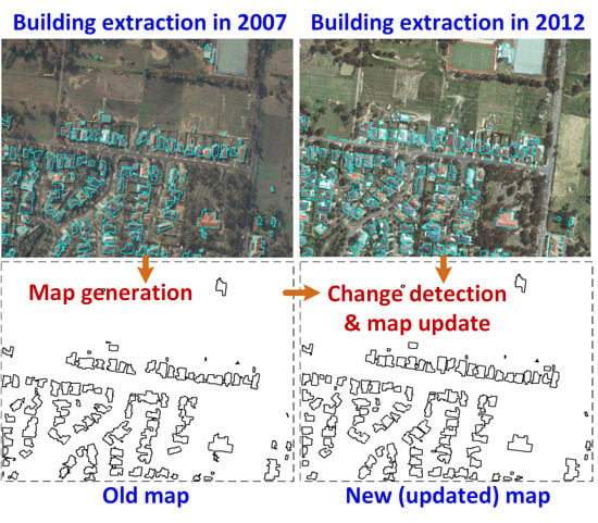


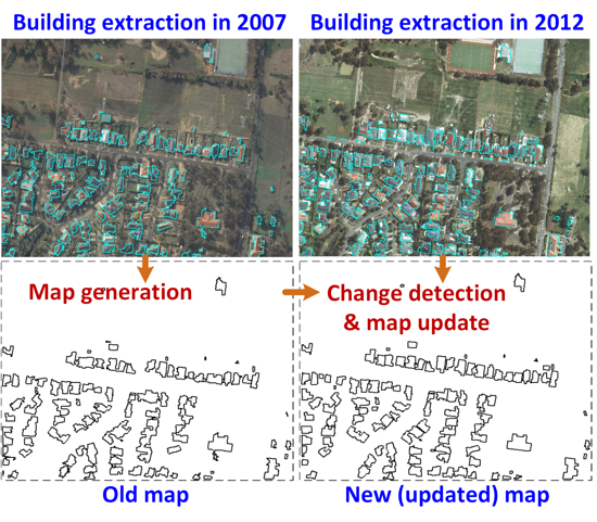
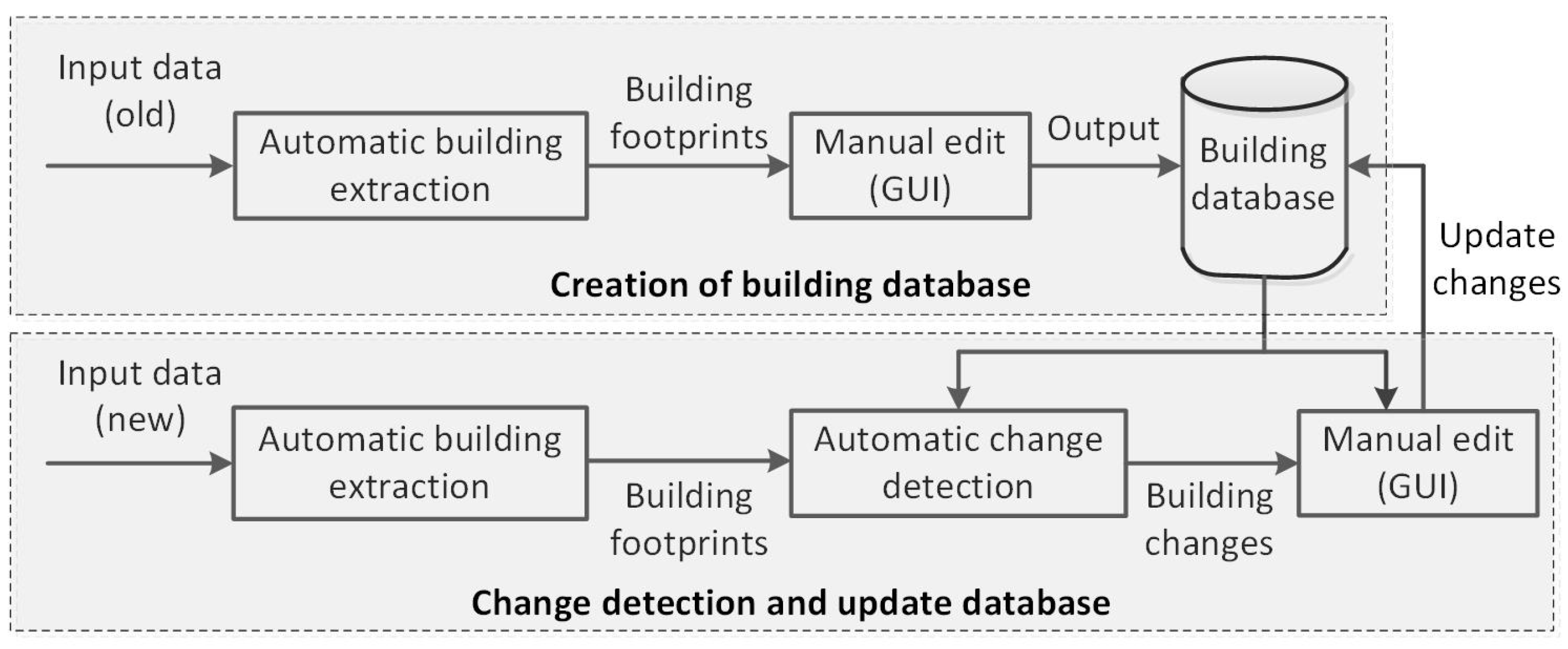
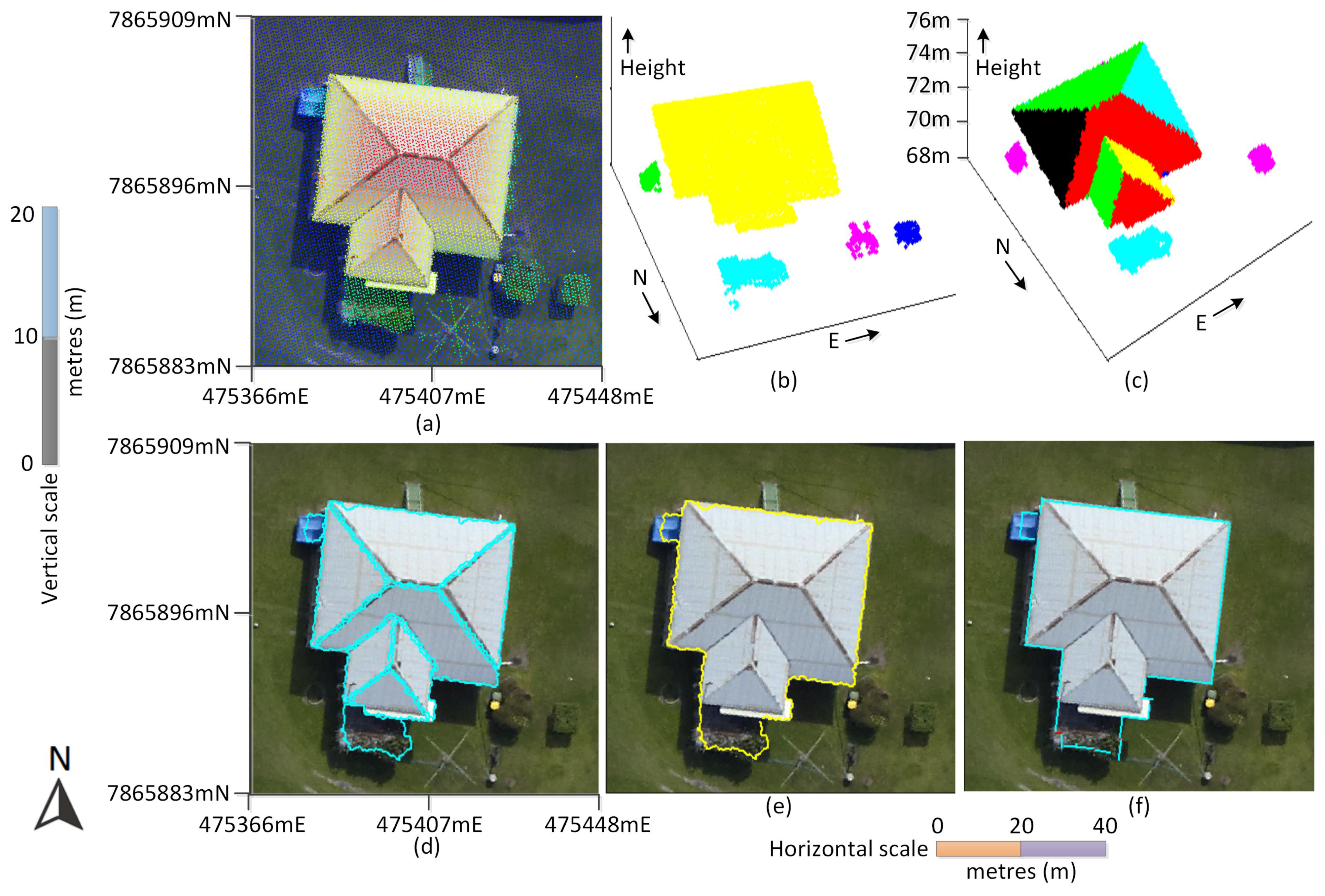
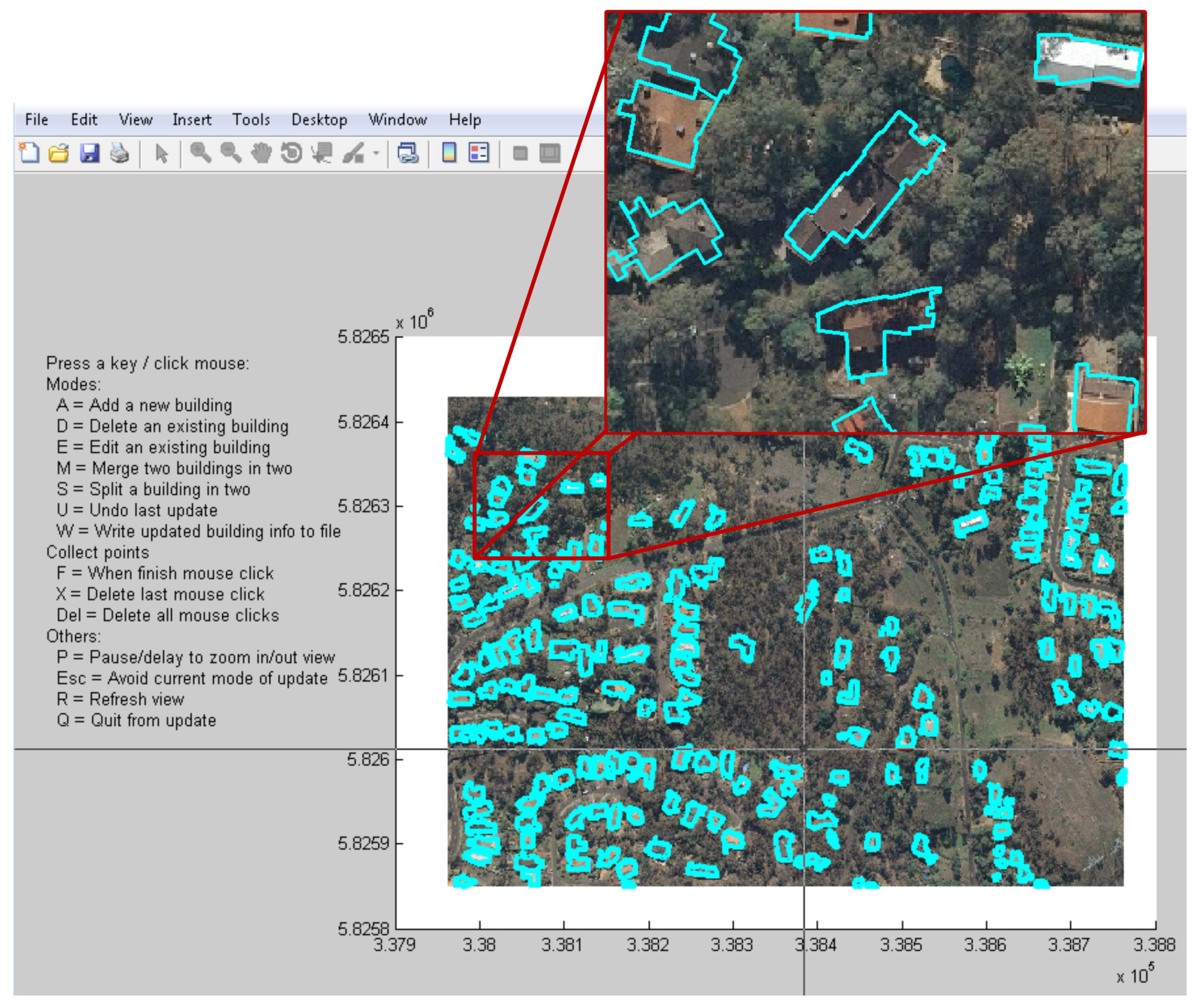
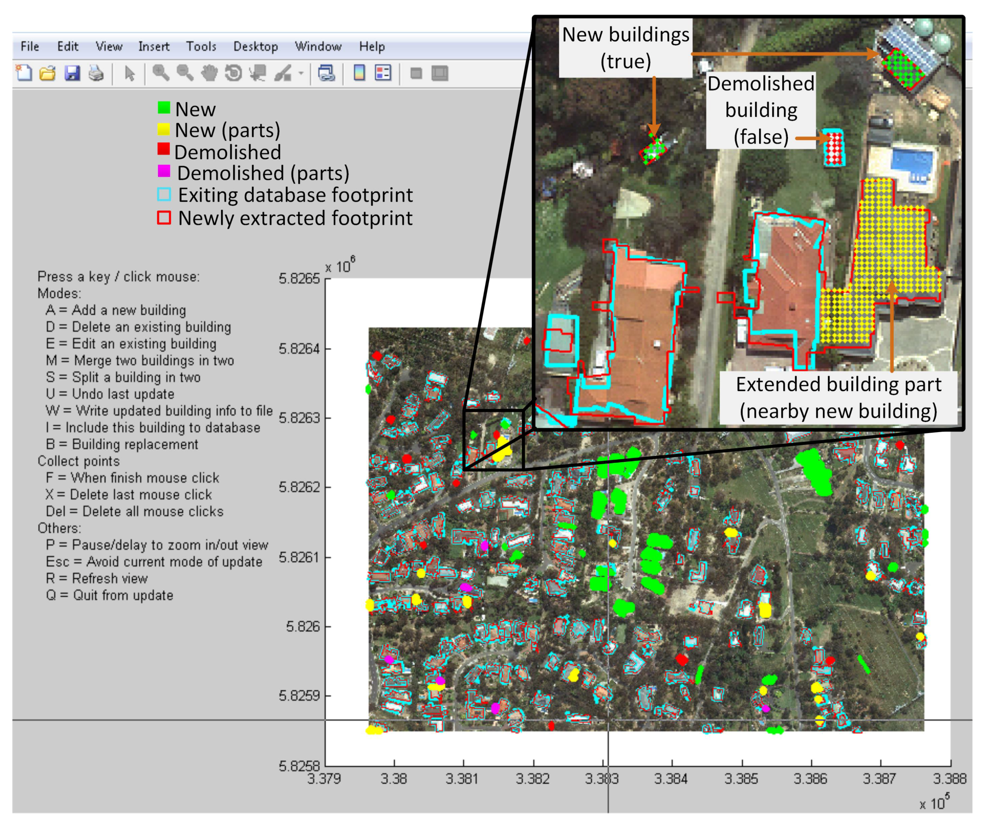
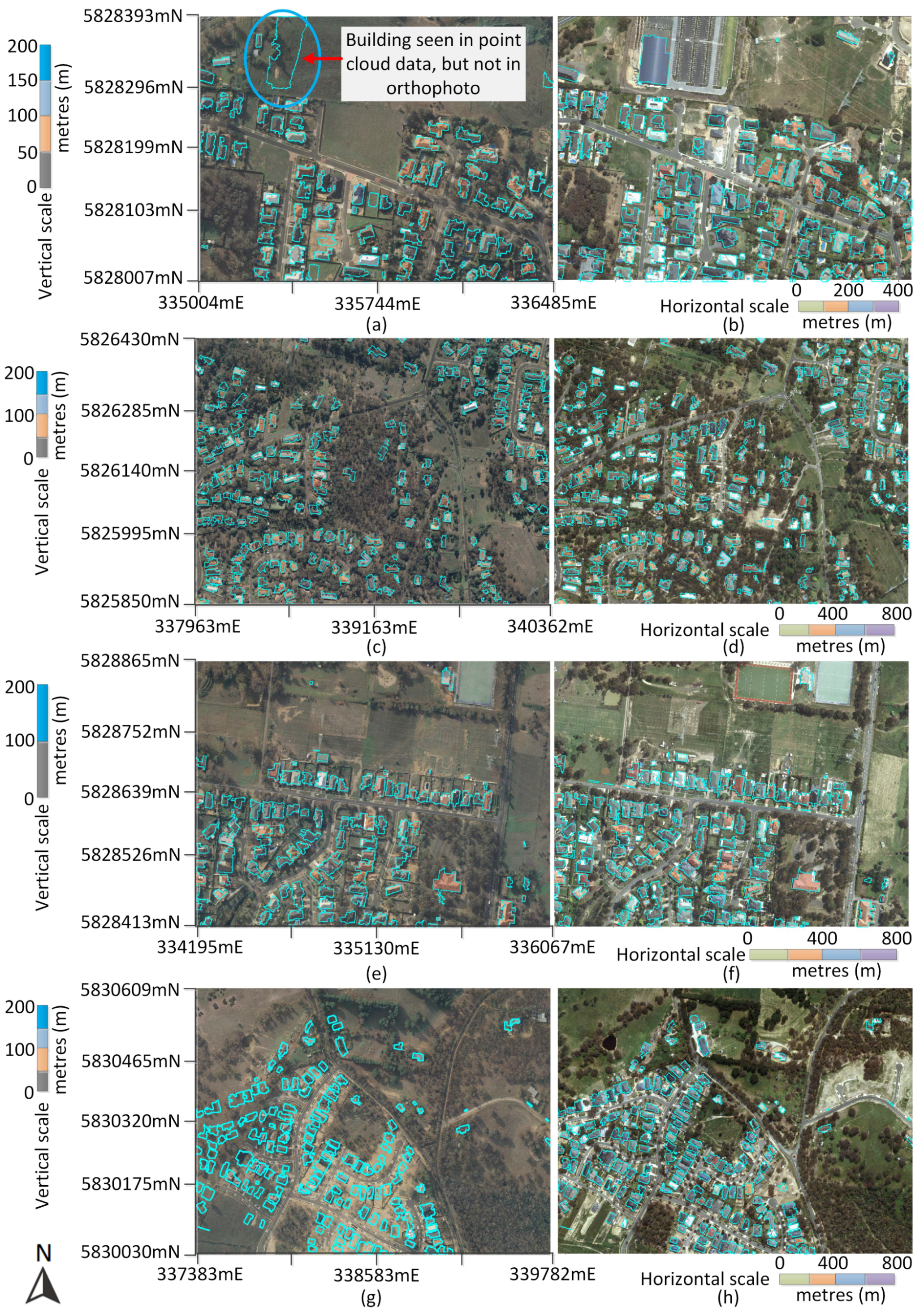
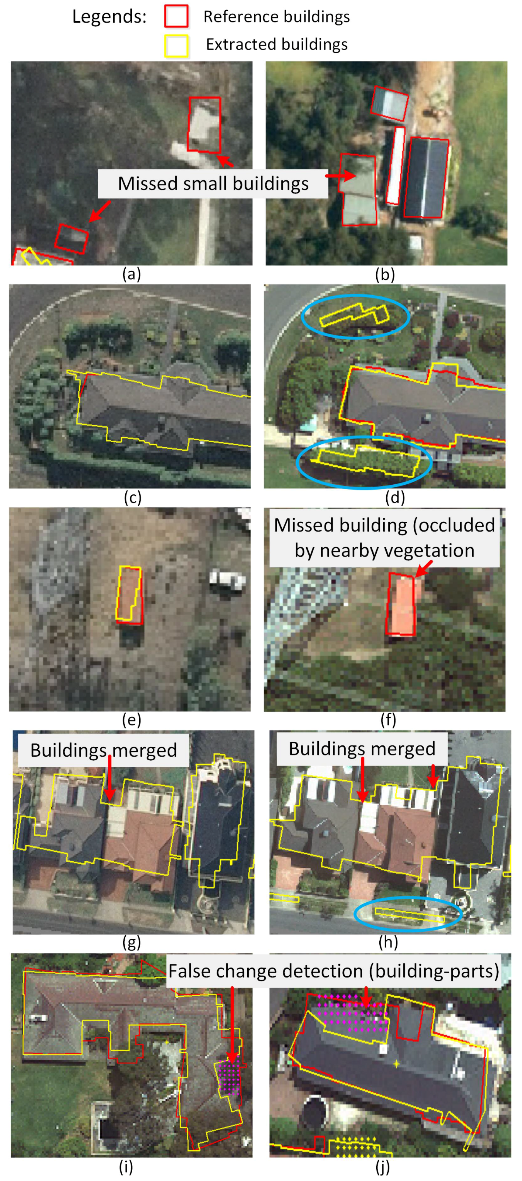
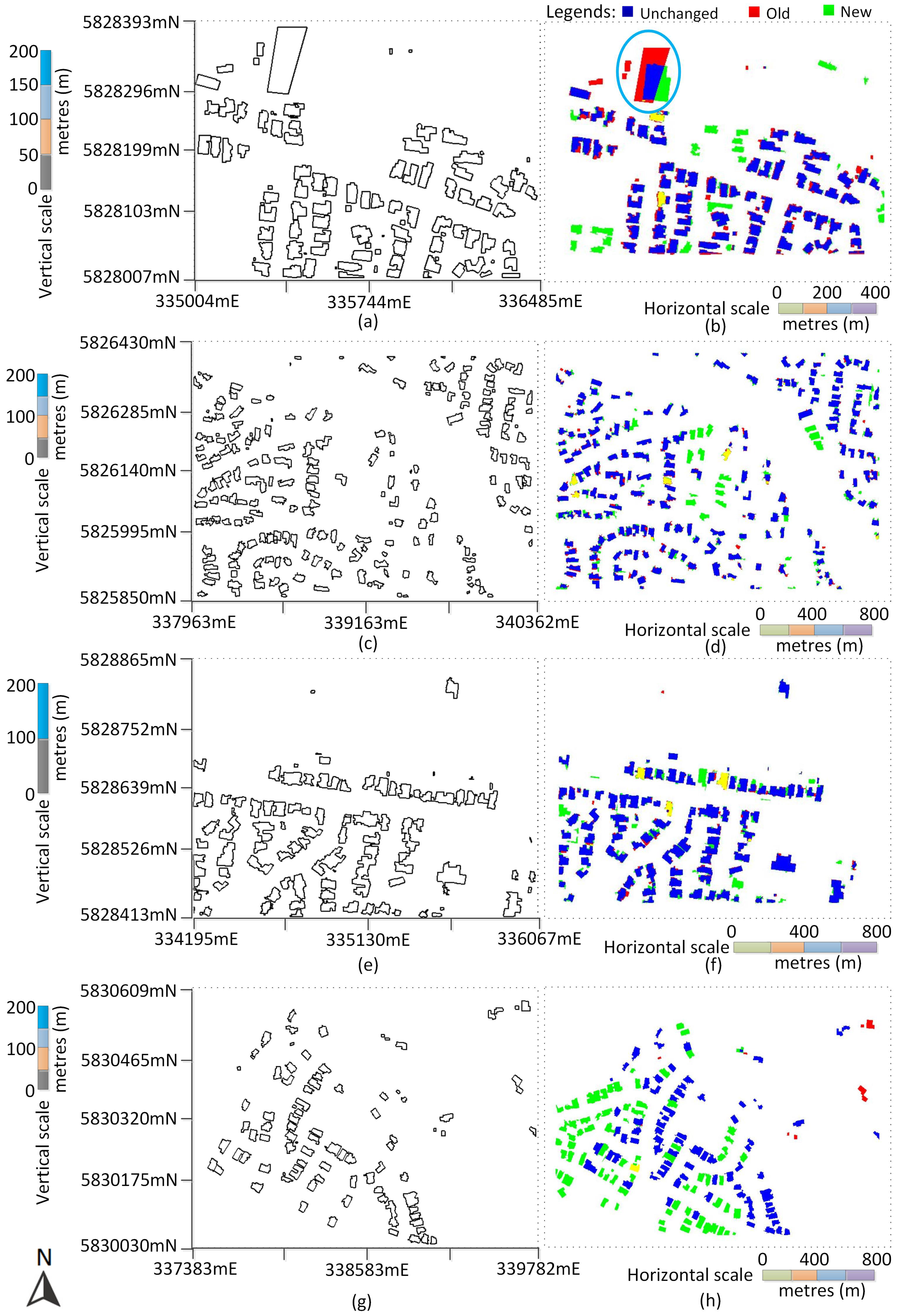
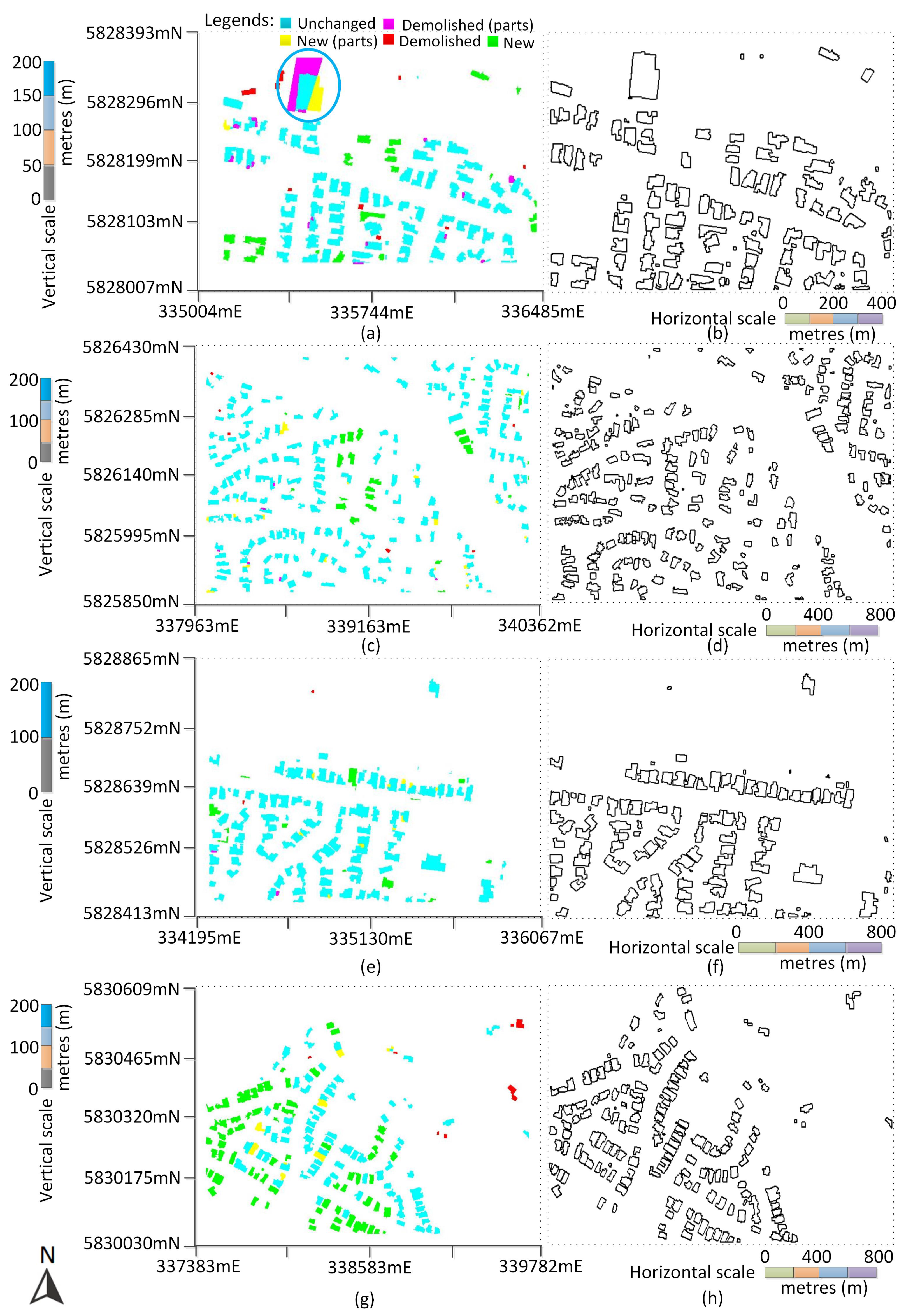


