1. Introduction
Morphotectonic analyses (especially channel offsets) along active strike slip faults are powerful tools to infer parameters such as segmentation, slip-rate, slip per event, and recurrence of earthquakes. Hazard assessment depends on this information and its uncertainty. Research activity on this topic has focused on (1) slip per event along fast-moving faults (e.g., [
1,
2,
3,
4,
5]); and (2) long-term slip-rates along lower slip rate faults [
6,
7,
8,
9,
10,
11,
12,
13,
14]. The distinction between them largely comes from the potential for separating the contributions of individual earthquakes to the measured offset, which is higher in the case of rapid slip and recurrence rate and low surface process rates.
The first group of studies shows an along-fault distribution of offsets including quality ratings. Recent surface fault ruptures leave their imprint in the geomorphic record thus individual fault rupturing events may be identified (e.g., [
1,
2,
4,
5]). In the second group, studies typically have measured offset terrace risers (e.g., [
11,
15]) or channels on alluvial fan surfaces (e.g., [
9]) with numerical age control to determine slip rates at the 10
3–10
4 year timescale. One example of this second group is [
6]
, which systematically analyzes the distribution of 300 measured offsets along the Kunlun (China) fault. The secondary aim of the long-term slip-rates studies for slow faults is to relate the formation age of the measured features with known regional or global climatic events. The long-term slip rate studies typically do not characterize offsets according to the quality of the measurement, with some exceptions [
10]. In general, measurement uncertainties are expressed as a range in the plausible retrodeformation [
7,
11].
It is necessary to make a distinction between the measurement uncertainty and its quality. Aleatory uncertainty is that associated with the measurement process itself, whereas the epistemic uncertainty describes the degree of ambiguity in the interpretation of the offset history of the feature [
16,
17]. There is no standard methodology to rate the quality of offset landforms (largely ascribed to epistemic uncertainty). Most approaches (all of them developed for fast-moving faults) define a subjective, qualitative rating (
i.e., excellent, good, fair, poor) based on landform projections and fault trace delineations as controlling the offset reconstruction (e.g., [
2,
17]). For example, [
5] score between 0 and 1 according to the degradation of the landform and the obliquity between the fault and the channel. This range (0 to 1) allows them to weight the Probability Density Function (PDF) of the individual offset measurement. After that, they sum the individual weighted PDFs along a specified fault reach to obtain the Cumulative Offset Probability Density (COPD; [
18]). The COPD may be used to identify the offset sequences tied to successive earthquake ruptures (e.g., [
2,
3,
4,
5,
18,
19]). Van der Woerd
et al., [
6] also obtain a COPD for longer offsets, and they compare it to climatically driven geomorphic events, as climate variations modulate surface process rates and transitions [
20].
It is challenging to adapt this methodology to a slow- or moderate-moving fault. Single rupture events usually cannot be identified in the geomorphic record because they have been smoothed by surface processes. Although the measured offsets are in general large (tens of meters; being the accumulation of several small offsets along time), the ability to identify them decreases with the dimensions of the offset [
1,
3,
6]. This is obvious in offset histograms which show an exponential decrease of the number of identified elements with larger offset magnitudes [
3,
8,
19]. Despite these obstacles associated with the potentially ambiguous landscape record of the superficial effects of slow-moving faults, their hazard assessment is essential [
21,
22].
In this paper, we adapt some of the approaches applied to small and few-event offsets along rapidly slipping faults to characterize the activity of low slip rate faults. We thus present a new methodology for scoring offsets and we apply it to a slow-moving strike-slip fault (the Alhama de Murcia fault, SE Iberian Peninsula) to refine our understanding of the hazard it poses and to illustrate our approach. We apply the scoring to the 138 offsets we identified as part of this study along the Alhama de Murcia fault. In the proposed methodology, we differentiate between subjective and objective scoring of quality and analyze effectiveness of the quality metrics. From the summary scoring, its distribution along the fault zone, and the distribution of these offsets, we calculate COPDs along strike of the Alhama de Murcia fault and evaluate potential segment boundaries and variations in slip rate. Additionally, we explore possible associations of entrenchment periods with the climatic cycles.
2. Geological Setting
The Alhama de Murcia fault (AMF) is a left-reverse strike slip fault [
23]. It is one of the structures in the Eastern Betics Shear Zone (
Figure 1; together with Carboneras, Palomares, Carrascoy and Bajo Segura faults), which absorbs the convergence between Eurasian and African plates (
Figure 1; [
24,
25,
26]). The most significant historical earthquakes (intensity ≥VII EMS) in the study area were in 1907 in Totana and in 1579, 1674 (VIII EMS) and 1818 in Lorca [
27]. The largest instrumentally recorded earthquake occurred in Lorca on 11 May 2011, had a moment magnitude of 5.2, and VII EMS intensity [
28]. The foreshock of this earthquake had a moment magnitude of 4.5 and the focal mechanism of the event shows oblique reverse faulting [
28]. No surface rupture in this seismic event has been identified.
The AMF has been segmented based on fault trace geometry, orientation (it varies N45–65E), trace complexity, seismicity, and geological history (
Figure 1; [
29]). From south to north, the segments are: (1) Huercal Overa-Lorca, ending in the south in a horse-tail (formed by two subsegments whose subdivision is in Rambla de los Pintados); (2) Lorca-Totana, where the fault splits into several sub-parallel fault traces; (3) Totana-Alhama de Murcia; and (4) Alhama de Murcia-Alcantarilla, where the geomorphic manifestation of the fault is diffuse. The southern ending of the fault is in a tiny district belonging to Huercal Overa, named Goñar, but we will refer to it as Huercal Overa (
Figure 1).
Although the main sense of motion along the fault is considered to be left-lateral, details of its slip sense are not well known. Morphotectonic studies describe left-lateral channel offsets [
30,
31] and infer a left-lateral slip-rate of 0.21 mm/year with undetermined uncertainty [
32]. GPS velocities from the region [
33] show that these values might be minimal, as they imply up to 1.5 mm/year horizontal slip-rate along the Alhama de Murcia and Palomares faults. Paleoseismic studies suggest a component of dip-slip at 0.04–0.35 mm/year for the upper Pleistocene in the Lorca-Totana segment [
25,
32], and 0.16–0.22 mm/year for the horse-tail termination in Huercal Overa-Lorca segment [
34]. Preliminary results from 3D excavations and subsurface restorations along the Lorca-Totana segment suggest larger left-lateral slip-rate values, higher than 0.62 mm/year and probably around 1 mm/year [
35].
Figure 1.
Geological setting of the Alhama de Murcia fault (AMF). Explanation: CF, Carboneras fault; PF, Palomares fault; CAF, Carrascoy fault; BSF, Bajo Segura fault. Inset modified from [
36]. Southern segments of AMF and 3D excavation site [
25,
32] are highlighted. The studied area is covered by the lidar topography-derived DEMs (hillshade basemap). AMF segmentation: (1) Huercal Overa-Lorca segment, (1.1) Huercal Overa-Rambla de los Pintados subsegment; (1.2) Rambla de los Pintados-Lorca subsegment; (2) Lorca-Totana; and (3) Totana-Alhama de Murcia. Segment 4 (Alhama de Murcia-Alcantarilla; not shown) is beyond the limit of the lidar to the northeast of Segment 3. Locations of offset examples are presented by the points REF025, REF036 and REF093.
4. Proposed Methodology for Assessment of Cumulative Offset Markers
Inspired by existing scoring criteria for offsets along rapidly slipping faults [
2,
5], here we propose a more detailed way to rate offsets along low slip rate structures such as the AMF. We have divided the presentation into three parts. The first is the measurement
versus uncertainty relationship, well expressed in the Probability Density Function (PDF) of each offset. We then propose differentiation of the quality scoring in two parts: (A) the subjective quality, which expresses the general confidence of the offset in terms of general geological knowledge; and (B) the objective quality, which is described in terms of three measureable geomorphic parameters (lithological changes, associated morphotectonics and shape). Both qualities have values between 0 and 1 and thus can be used for relative weighting of offset PDFs.
We apply this methodology to AMF along which we have identified and measured 138 left lateral offset features (.kmz file in the
Supplementary Material), mainly stream channels (three ridge lines; from now on, we will refer to all features as channels, in general). The measurements and quality ratings were made by the first author, with cursory review from the other two authors. This rich and consistently measured and rated dataset has value for characterizing the Quaternary activity of the AMF (e.g., [
25,
36]), but also serves as a validation test of our proposed methodology.
4.1. Measurement and Uncertainty Relationship
Measuring the offset of a feature requires an estimate of its pre-deformation morphology [
19]. In general, more than one piercing line can be defined (near and full channel projections; [
10]). For the AMF offset dataset, we measured all possible combinations of piercing lines of landform elements (including channel rims,
Figure 2). We compute mean and mean standard deviation for all the measurements (from two to nine measurements) obtained for the given feature. Mean and mean standard deviation define the Gaussian probability density functions (PDF). Mean standard deviation is 68.3% or 1σ of the PDF.
The relationship between the amount of displacement and the horizontal uncertainty in our AMF dataset do not follow the same proportionality for all features (
Figure 3; that is, big offsets do not necessarily have big uncertainties and small offsets, small uncertainties) [
17]. Extrapolate a logarithmic relation for uncertainty and offset.
4.2. Subjective Quality
The subjective quality score represents the individual confidence of the geologist when considering each offset. Inspired by [
5], its values range between 0 and 1, where 0 is very low quality, 0.25 is low quality, 0.5 is medium quality, 0.75 high quality and 1 very high subjective quality. The experience of the geologist influences the rating [
17]. Bond
et al. [
38] and Bond
et al. [
39] show that experience may be a big bias (availability, anchoring, and confirmation) when measuring. Incorrect geological interpretations may result if the conceptual model does not agree with reality. In that sense, experts tend to interpret geological data according to their expertise and previous knowledge (conceptual uncertainty) and they may not show a high confidence about their interpretations. Salisbury
et al. [
4], Scharer
et al. [
16], Salisbury
et al. [
17] and Bond
et al. [
38] propose that the results are better when more techniques are used to approach the problem (multiple approaches to measurement both remotely and in the field in the offset landform case).
Figure 2.
Schema used to define piercing lines (elements) and measure the offset of a channel crossing a sinistral fault (red line with arrows). Black lines are the rims of the channel and blue line is the channel thalweg. Piercing lines are defined for rims and thalweg separately and we consider near and longer length feature projections (solid and dashed). Letters indicate the channel feature taken into consideration and numbers refer to the number of measurements done with all possible combinations of piercing lines for each channel feature (rims and thalweg).
Figure 3.
Relationship between offset and uncertainty for the 138 offsets measured along the Alhama de Murcia fault. Horizontal axis is the mean offset value for each feature (PDF mode), vertical axis is the mean standard deviation.
Figure 3.
Relationship between offset and uncertainty for the 138 offsets measured along the Alhama de Murcia fault. Horizontal axis is the mean offset value for each feature (PDF mode), vertical axis is the mean standard deviation.
4.3. Objective Quality
The aim of this section is to suggest a scoring approach for geomorphic and geologic aspects of the offset feature, which influence our ability to reconstruct it. We name it “objective quality” because its rating relies on objective (but potentially arbitrary) repeatable metrics to minimize the inherent bias in the subjective quality. However, a minimum knowledge of geology is required.
Six parameters can describe an offset: (1) type (if the channel is entrenched in the basement or in an alluvial fan surface, or we are measuring a ridge line); (2) present-day preservation of the feature; (3) associated age control (absolute, relative or none); (4) lithological changes (if the fault coincides with a rock type change); (5) associated morphotectonics (the number of morphotectonic features spatially related with the analyzed feature); and (6) shape, which depends on three sub-parameters (fault zone width, difference in orientation between the two segments of the channel, and sinuosity;
Table 1). The first three shape parameters cannot be easily and consistently scored in terms of objective quality. Nevertheless, they are useful for initial characterization during field or remote fault trace investigation. We move forward with the latter three parameters (objective quality metric parameters;
Table 1) as contributors to an index of objective quality ranging from 0 to 1.
Table 1.
Objective quality metric parameters (lithological changes, associated morphotectonics and shape) summary description.
Table 1.
Objective quality metric parameters (lithological changes, associated morphotectonics and shape) summary description.
| Parameter Name | Description |
|---|
| Lithological changes | Fault coincides with a rock type change which controls resistance to erosion |
| Associated morphotectonics | Morphotectonic elements spatially related (Figure 4) |
| Shape | Depending on 3 sub-parameters: fault width, orientation of the channel, and sinuosity (Figure 5) |
4.3.1. Lithological Changes
The feature receives one point if the rock
type where the channel is entrenched is homogeneous and 0.5 points if the fault coincides with a lithological change. Where the fault puts in contact two different rock types, it is easier to map the fault line scarp. The purpose of this parameter is to represent the possibility of a stream changing its direction because of differences in resistance to erosion of the geologic material rather than active faulting.
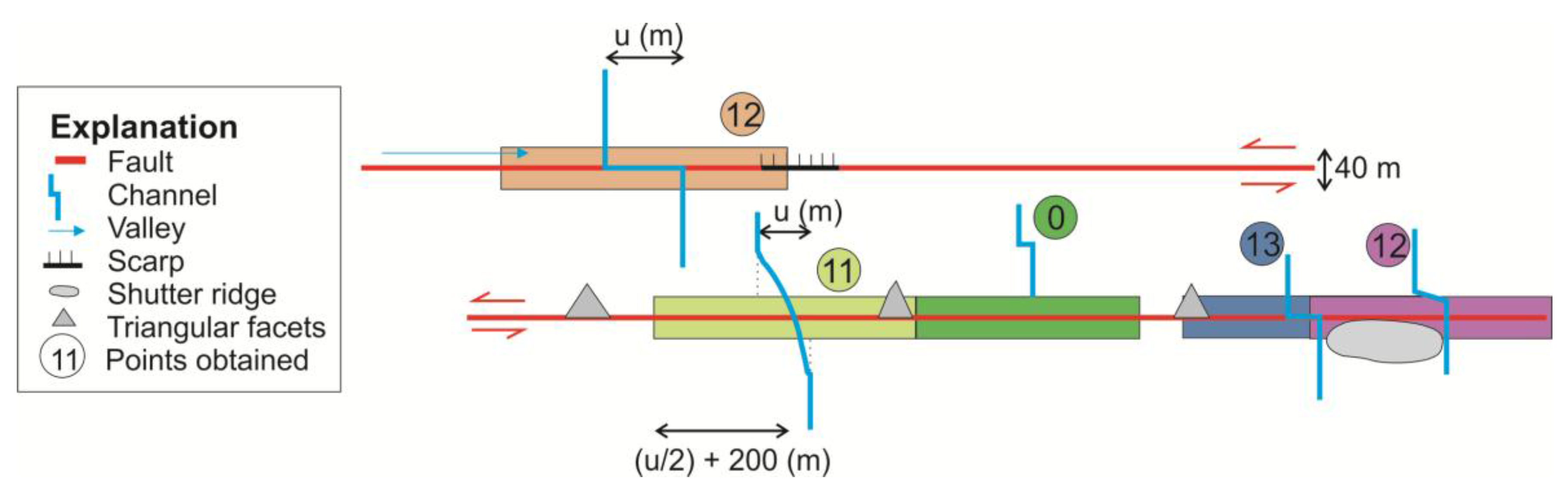
4.3.2. Associated Morphotectonics
This parameter reflects the number of other spatially-related morphotectonic features in the vicinity of an offset feature. The significance of an offset feature increases with the presence of others nearby to indicate the consistency of the assignment of fault activity to any given feature. Klinger
et al. [
3] use a similar approach in which they count the number of elements reconstructed using a certain amount of back-slip within 100 m of a specific offset feature. The rating they give to every feature is the number of coinciding elements.
Inspired by [
3], our goal here is to score the feature between 0 and 1 by considering the presence of associated morphotectonic features. Thus, we propose a modification of their methodology. For each feature, the region for identifying spatially-related morphotectonic elements is defined by the intersection between (1) the approximate mean width of the fault trace zone along the entire fault; and (2) a circle around the central point of the feature that has a radius of half of the offset measurement plus 200 m (
Figure 4). This modification is appropriate for more geometrically complex fault traces such as those along the AMF. For the AMF, we chose 40 m for the fault zone width because it is an intermediate value between the approx. 20 m of fault zone width observed in the 3D trenches [
35] and the approx. 100 m of fault gouge in a geophysical borehole [
40].
The specification of the search radius around every feature was defined after comparing the values obtained for four different lengths (
Figure S1). The candidate radii were: (1) ten times the offset; (2) the mean offset plus 100 m; (3) the mean offset plus 200 m; and (4) half of the mean offset plus 200 m (
Figure S1). For the three first cases, the radius depends too much on the offset, especially for the first one, whose dimensions for big offsets do not match any geological criteria. Although it is the search radius used by [
3], the 100 m search radius for Alhama de Murcia fault is too small. The fourth option (half of the mean offset plus 200 m) is our final choice because the influence of the offset measurement on it is lower and the addition of 200 m to the radius makes sense along a slow moving fault given the interplay between surface processes and fault activity.
Each offset feature receives 10 points if its deformation occurs within the fault zone, and one extra point for every morphotectonic feature set inside the area of intersection. The considered morphotectonic elements are: (1) another offset channel; (2) fault parallel valleys; (3) scarps; (4) triangular facets; and (5) shutter ridges. The related feature need not be completely within the intersection zone to score (
Figure 4). In places where the fault is comprised of more than a single fault trace, the search area takes into account just those elements related to the fault trace that offsets the considered feature (
Figure 4). The maximum points we obtained for the AMF offsets are 16. As it is required that the associated morphotectonics score ranges between 0 and 1, we thus divided the points obtained for every feature by 16.
We are aware of the arbitrariness of this parameter. In fact, the final scoring depends basically on how many morphotectonic features are mapped. This mapping is subjective, especially along slow or moderately-moving faults where the geomorphology related to the fault activity may be weakly evident. Nevertheless, we use this parameter in the objective quality because the consideration of a feature to be analyzed also must take into account the associated mapping uncertainty.
Figure 4.
Illustration of the associated morphotectonics scoring for the AMF. The defined boxes are the intersection area between the width of the AMF fault zone (40 m) and the search radius circle around the central point of the feature of half of the offset measurement (u) plus 200 m. Each offset is indicated by the different colored boxes and circled point score. For example, the uppermost (orange) feature has 12 points because the deformation occurs within the fault zone and there are two morphotectonic features (fault parallel valley and scarp) spatially related with it.
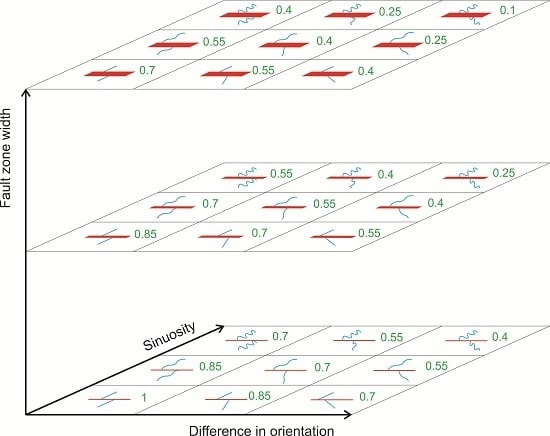
4.3.3. Shape
The shape parameter can be decomposed into three sub-parameters: (1) fault zone width; (2) angular difference in orientation between the two parts of the considered feature (on either side of the fault); and (3) sinuosity of the channels.
Figure 5 illustrates the rating according to the three sub-parameters (modified significantly from [
17]). Every time one sub-parameter decreases one step along its axis, the value of the final shape scoring decreases 0.15 (
Figure 5). The three sub-parameters can be considered separately, as well. In this case, every step of increase sub-parameter represents 0.45 points of decrease in the value of its scoring. For example, sinuosity would take ratings 1, 0.55 and 0.1 as it increases. The shape scoring would be the same when considering them (fault zone width, sinuosity and difference in orientation) separately, as values and decrements are proportional.
Figure 5.
Offset shape rating. Three axes represent shape sub-parameters: fault zone width, difference of orientation of the two segments on each side of the fault and sinuosity. Blue lines are the channels, red lines are the fault zones (thickening with width), and green numbers are the shape scoring for every combination of the sub-parameters. Keeping two of the axes constant, shape rating decreases 0.15 points every step in the other axis, making it possible to have values between 1 and 0.1.
4.4. Final Scoring of Objective Quality
The final score of objective quality is an average of the three parameters, taking into account that “shape” is composed by three sub-parameters, where
a is lithological changes,
b is associated morphotectonics and
c is shape (Equation (1)). The shape parameter is multiplied by three because in fact it is made of three sub-parameters. This way, we weigh the real contribution of the three sub-parameters composing “shape”.
7. Implications for Active Tectonics Investigations
In this section, we examine the distribution and degree of offset clustering of the measured offsets along the AMF to infer fault segmentation and slip rate. The measured offsets (with their uncertainty) along the fault show no evidence of offset clustering (
Figure 12). There is no evident relationship between any type of quality and the location along the fault. The histogram in
Figure 13A displays no clustering, but it shows the previously suggested offset identification decay with the length of the offsets (e.g., [
1,
3,
6]). This histogram accounts for measurement uncertainty for each offset. In order to obtain clear clusters of amount of offset, we follow the methodology developed by [
5] (originally demonstrated by [
18]). We sum the individual PDFs (
Figure 13B) to produce a COPD with several peaks (
Figure 13C). These peaks represent amounts of offset measured with more frequency along the stacking reach (
Figure 13C). No clear regularities in the peak position and in the distance between peaks are observed. As expected, we cannot identify individual seismic events, in contrast to what is possible along fast-slipping faults [
2,
5]. Moreover, accounting for objective and subjective qualities, two additional weighted COPDs are produced (
Figure 13D). We weighed the area of every individual PDF with the subjective and objective qualities (
Figure S2). This results in two curves with lower and missing peaks compared to the initial COPD (
Figure 13D).
Figure 12.
Offset geomorphic features along the Alhama de Murcia fault. Error bars represent uncertainties (mean standard deviation values, 1σ). Scoring for both subjective (
upper plot) and objective (
lower plot) quality are represented with different symbols. Objective or subjective quality legend: [0–0.25), very low quality; [0.25–0.5), low quality; [0.5–0.75), median quality; [0.75–1], high quality. No clusters on the amount of offset are evident in these plots. The AMF trace and its segmentation (see
Figure 1 for numbers explanation) are shown at the bottom of the figure.
The COPD of all of the data (
Figure 13C,D) does not take into account the characteristics of the individual fault segments (
Figure 1). Even if we assume that all the fault segments have the same characteristics (e.g., slip-rate), where the fault is composed of several fault traces, the individual parameters will vary. Therefore, we do the same analysis considering individual segments and individual fault traces (
Figure 14). COPDs are computed for Segments 1.1 (Huercal Overa-Rambla de los Pintados), 1.2 (Rambla de los Pintados-Lorca) and 3 (Totana-Alhama de Murcia) where the fault is a single trace; and for segments where the fault splays: (a) three fault traces in the horse-tail termination; (b) the sub-parallel traces in Segment 2 (Lorca-Totana); and (c) for two traces in the Totana-Alhama de Murcia segment (Segment 3).
Figure 13.
(A) Histogram of the offsets and uncertainties. (B) Individual Probability Density Functions (PDF) of all features along the fault. (C) Cumulative Offset Distribution Probability (COPD) with no weighting and peak values highlighted. (D) COPD weighted previously with subjective (green) and objective (blue) quality score. Notice the difference in the vertical axis in the probability values (B–D). In general, the subjectively weighed COPD (green line) is lower than the objective COPD (blue line).
The COPDs enable the identification of groups of offset features along the entire fault and by segments. We assume that the stacking of individual PDFs reinforces signals of common offset along analyzed fault reaches. Although fault segments usually are classically defined by geological, geomorphological and geophysical observations and inference [
30,
31], the analysis of the COPDs may provide additional information on common amounts of offset further refining the location of segment boundaries and possibly highlighting slip rate variability between segments. To explore if all segments of the fault have the same slip-rate, we assume that all the features with the same offset were entrenched or formed at the same time, and thus, due to fault activity, they display the same amount of offset.
The COPDs of fault segments and traces are clustered. The best example is fault trace 2.2, where 15 offset features cluster in four peaks. Clustering is also evident along fault Segment 1.1 (three offsets in two peaks), in fault traces 1.11 and 3.2 (6 offsets in 4 peaks) and in fault trace 2.3 (28 offsets in 10 peaks).
Figure 14.
Individual non-weighted COPDs for the considered fault segments and fault traces (see text). The fault trace that corresponds to every COPD is indicated by number. Alhama de Murcia fault segmentation according to [
29] (see
Figure 1 for location and explanation). In brackets, the number of measurements involved in every COPD.
The first comparison between COPDs is made between Segments 1.1 and 1.2 (Huercal Overa-Lorca sub-segments). Two peaks coincide in these segments: (a) 42 ± 17 (Segment 1.1) and 56 ± 4 (1.2); and (b) 99 ± 5 (Segment 1.1) and 107 ± 14 (1.2). Despite the identification of only three offsets along Segment 1.1 (Huercal Overa-Rambla de los Pintados), the two common modes between Segments 1.1 and 1.2 support an inference that both sub-segments have the same slip-rate. Thus, there may be no need to divide the segment Huercal Overa-Lorca in two, as other geological data suggest [
29,
36].
The second comparison is done between Segments 1 (Huercal Overa-Lorca) and 3 (Totana-Alhama de Murcia). The low geomorphic evidence of Segment 3 (only two offsets where the fault is expressed as a singular trace) limits the comparison. Thus, the coincidence between the peak in 252/257 m is not a sufficient condition to suggest that both segments have the same slip rate, because there are no other geological evidences.
The last general comparison is between sub-parallel fault traces within the same segment. The first case is the southwestern end of Segment 1 (Huercal Overa-Lorca) characterized by a horse-tail termination [
30,
31,
34], where the COPDs along the fault traces show no common modes. Similarly, mismatched peaks exist for the traces (traces 3.1 and 3.2) in Segment 3 (Totana-Alhama de Murcia). We infer that variations in orientation of the individual fault traces within these zones result in accommodation of different amounts and styles of deformation, possibly resulting in slip rate variability.
Segment 2 (Lorca-Totana) has three fault traces (2.1, 2.2 and 2.3) along most of its length. The orientation of the segment (N 45 E) differs from the orientation of the other segments (N 65 E). This change in strike results in a higher vertical component of slip which may promotestream entrenchment [
41]. As the slip here is divided in three fault traces, we cannot compare this segment with the others. Along strike of Segment 2, the four peaks of the COPD of fault trace 2.2 (10, 31, 98 and 202 m) coincide approx. with the amount of offset of the peaks 8, 32, 98 and 194 m in trace 2.3. According to our assumption (segments with similar COPDs have the same slip rate), fault traces 2.2 and 2.3 would thus slip at a similar rate. However, a geological criterion suggests that fault trace 2.3 has a higher slip rate, as its geomorphic expression is sharper (recent paleoseismic excavations, [
25,
32]). Thus, even if the entrenchment occurs at the same time along each of the traces, fault activity influences the number of preserved accumulative offsets.
In summary, the COPD analysis supports the previously defined fault segments, but the analysis should be done for fault segments with sufficient offset features identified along them. Fault segments that differ in orientation cannot be compared with the COPD, as deformation is absorbed in a different way (for example in segment Lorca-Totana). The analysis of the COPD allows relative comparison of the slip rates along the segments. It is not possible to calculate the slip rate by itself (this point is discussed in section 8). Moreover, even with good correlation, the coincidence of clusters between fault segments is not a sufficient condition to confirm that two fault traces have the same slip-rate as other geological criteria have to be taken into account (i.e., geomorphic expression and paleoseismological results).
8. Entrenchment Correlation with Climate Variation
The main control in the relationship between erosion and accumulation in a fluvial system is the amount of protective vegetation cover in the area, and this varies with climate (strongly argued by [
20]). Bull [
20] do not specify which type of climate changes cause the loss of plant cover. Some authors relate alluvial fan aggradation with interglacial stages [
6,
14]. Alternatively, based on soil dating in SE Iberian Peninsula, [
42] concluded that sedimentation occurs during glacial stages due to landscape instability. Their results indicate that climate during glacial stages in the southeastern Iberian Peninsula is apparently cold and dry, suggesting that climatic characteristics may vary regionally within individual marine isotope stages.
In this section, we explore the correlation between COPD with climatic curves to explore preferential climate channel entrenchment in the region. This information may be used in the future as a proxy to indicate the age of sedimentary units in which channels have entrenched, especially in a site where numerical dating is challenging. To do that, we assume that climatic variations triggered channel entrenchment synchronously across the region. If this assumption is correct, the channels (along the same fault segment) that were entrenched at the same time should display the same amount of offset. The peaks in the COPD for that segment represent these amounts of offset. As climatic events are well represented in the climatic curves, we compare the COPD with them [
6]. This comparison has to be done with age control. In this test, we also consider other causes for channel entrenchment such as pulses of uplift.
Several authors have related known ages of depositional units (related to offset features) with climatic events [
6,
8,
11,
14]. In general, few offset features with age control are available to relate climatic events with entrenchment. Van der Woerd
et al. [
6] have well constrained ages of the (<20 ka) terraces into which the offsets are etched along Kunlun Fault (Tibet), and thus they compare the COPD with a climatic regional curve. They align the two equivalent portions of the curve and then extrapolate the ages to the largest offsets assuming a constant slip-rate of 11.5 mm/year. Moreover, they assume that the deposition of the dated fluvial terraces and the entrenchment happens always in interglacial periods because during glacial times that area is covered by ice. Chevalier
et al. [
11] analyze terraces as well, following the same methodology that [
6] used, but their geological units are much older (up to 200 ka). They are able to correlate periods of fluvial deposition with interglacial periods along the Karakoram fault (>5 mm/year slip rate). Ferry
et al. [
8] analyze the offsets close to a lake. They correlate the age of the channels with known decreases of the lake level. Finally, [
14] do not have dated units but assume that the analyzed features were entrenched in interglacial periods in order to obtain the slip-rate for Idrija fault (1.5 mm/year).
The COPD and climatic curve (e.g., δ
18O or paleotemperature) can be also compared according to the position of their peaks or troughs if we assume that the channels entrench synchronously with extreme of the climate proxy and a constant slip-rate. One problem we face when comparing the curves by their shapes alone is the attenuation of the geomorphic record (
Figure 13A; [
3]). The data for Alhama de Murcia fault presents the same decay relationship (
Figure 13), and thus we did not further pursue this approach (along with the tenuous underlying assumptions).
Age control along the AMF is limited; however, at least one age is necessary to align the climatic and the COPD curves (assuming a constant slip rate). We have just one numerical age [
25,
35] and a few relative ages [
30]. Moreover, the soil and landform chronosequence for the southeastern Iberian Peninsula is not well constrained [
43] and there are no more chronosequences for similar climates in the Mediterranean region. The preliminary results in 3D trenches (
Figure 1) show a buried approx. 15 ka channel (age determined by correlation with trenches in [
25]) that displays 15 m of offset [
35].
As there is just one absolute age, we use the relative ages as well. For offset features with the same relative maximum age (the maximum age of a channel is the age of the alluvial unit it is entrenched in), the feature with the largest amount of offset provides the maximum estimate of slip-rate (
Figure S3). As discussed in the previous section, not all segments have the same slip-rate. Thus, the comparison both COPD and climatic curves have to be done for the individual segments. Just one of the maximum slip-rates plotted in
Figure S3 belongs to a feature set in a zone where the fault displays a single trace (Segment 1.2, Offset REF095: 258 m in 200 ka).
The comparison between climatic and COPD curves is done in Segment 1 (Huercal Overa-Lorca) and in Segment 2.3 (Lorca-Totana) (
Figure 15). We employ the global sea level based on a benthic δ
18O curve constructed from 57 globally distributed records [
44] and regional curves (based on drilling cores in the Alboran Sea) of [
45] (benthic δ
18O curve) and [
46]. This last curve was constructed from planktonic δ
18O curve and it represents the mean sea surface temperature. This last curve is a good reference for regional temperatures.
Figure 15.
Correlation between the COPD (without weighting) of Segment 1 and trace 2.3 and climatic curves. Climatic curves are (1) the regional planktonic δ
18O curve in the Alboran Sea [
45]; (2) the regional mean sea surface temperature of the Alboran Sea [
46] and the benthic δ
18O global stack [
44]. For the Segment 1 (right side), the slip-rate of 258 m in 200 ka [
30] is used, whereas for trace 2.3, the approximate age obtained in the trenches (15 ka) for a 15 m buried offset channel [
35] is applied. Dashed lines represent slip rate constraints for each segment. Dotted lines indicate maximum glacial stages.
Along Segment 2.3 (
Figure 15), offsets appear to coincide with glacial to interglacial transitions. The younger age (15 ka) is from an erosive unit in the paleoseismic 3D-trenches [
35]. In this case, we are not correlating sedimentary units, but moments of erosion. Thus, we would infer that erosion is triggered by transitions from glacial to interglacial. We also infer that peaks that do not coincide with climatic events may be the result of entrenchment due to the small vertical component of deformation along Segment 2 [
25] or because of other stochastic processes.
Results from the comparison between Segment 1 COPD’s and climatic curve are less conclusive (
Figure 15). In this case, we align the curves using the relative age of a sedimentary unit. The estimated slip-rate is based on the offset of channel REF095 (offset 257 m) that is entrenched in an alluvial fan surface with a relative age of approx. 200 ka. The comparison suggests that maximum glacial stages coincide with periods of minimal sedimentation (
Figure 15), however this relationship is not clear. This apparent lack of correlation derives basically from the uncertainty associated with the relative age used to do the superposition of the curves. However, the aforementioned correlation of lack of sedimentation during glacial stages, agrees with suggested by other authors [
6,
11] for other parts of the world, but disagrees with [
42] study in the SE Iberian Peninsula.
9. Conclusions
In this study, we propose a new methodology to score lateral offsets and we test it with a new offset dataset along the Alhama de Murcia slow-moving sinistral strike slip fault. We measured (amount of offset ± uncertainty, expressed as 1σ) every offset feature and we rated it in terms of subjective and objective quality (every quality can take values between 0 and 1). Six parameters represent objective quality, although just three of them can be characterized in terms of metrics (lithological changes, associated morphotectonics and shape). All the variables (amount of offset, uncertainty, subjective quality, objective quality, lithological changes, associated morphotectonics and shape) are apparently independent, except objective quality and shape whose correlation value is close to 1. This methodology is useful to characterize the offset feature catalog.
Cumulative Offset Probability Density (COPD) is calculated from the individual PDF (previously weighted by subjective and objective qualities). COPDs are a useful tool to compare fault segments. The coincidence of the COPD peaks’ position between fault segments is a necessary but not sufficient condition to ensure that the analyzed segments have the same slip-rate. COPD peaks of individual AMF traces show few coincidences between fault segments indicating that slip-rate may be different from one segment to the other, or that lack of data limits our results. Assuming that offset clusters observed in the COPD are entrenched at the same time, we test the possibility that entrenchment is triggered by climatic events. We compare the COPD with climatic curves to infer preferential climatic conditions for entrenchment. Along Segment 2.3 (Lorca-Totana), where we have some age control, channel incision may coincide with climatic transitions from glacial to interglacial stages. This approach may be used as a proxy for alluvial fan age, in order to calculate slip-rates for every fault segment.
Future work should be done testing this methodology for other faults. Another experiment is for the tectonic geomorphology along a fault to be analyzed by more than one geologist (see also discussion in [
17]). That way, we can compare the scores, and assess which variables depend most on the operator criteria. Moreover, efforts will focus on obtaining more numerical ages to decrease the uncertainties in the comparison between COPDs and climatic curves.


