
Remote Sensing of Storage Fluctuations of Poorly Gauged Reservoirs and State Space Model (SSM)-Based Estimation


Abstract
:
1. Introduction

2. Data and Pre-Processing
2.1. Changes in the Shoreline

2.2. Changes in Water Level

| Reservoir | Longitude (Degrees) | Latitude (Degrees) | Mission | Pass |
|---|---|---|---|---|
| Mead | −114.49 | 36.137 | Envisat | 0811 |
| Jason1 extended | 180 | |||
| Saral/Altika | 0811 | |||
| North Aral | 60.7489 | 46.5211 | Envisat | 0126, 0167, 0625 |
| Jason1 | 218, 107 | |||
| Jason2 | 218, 107 | |||
| Saral/Altika | 0126, 0167, 0625 | |||
| East Aral | 59.7146 | 44.9415 | Jason1 | 142, 107 |
| Jason2 | 142, 107 | |||
| Saral/Altika | 0670 | |||
| West Aral | 58.5626 | 45.1947 | Envisat | 0797, 0212 |
| Jason1 extended | 107 | |||
| Jason2 | 142 | |||
| Saral/Altika | 0797, 0212 |
2.3. Bathymetry
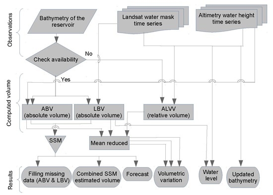
3. Methodology
3.1. Methods for Reservoir Volume Estimation
3.1.1. Altimetry-Bathymetry-Volume (ABV) Method
3.1.2. Landsat-Bathymetry-Volume (LBV) Method


3.1.3. Altimetry-Landsat Volume Variation (ALVV) Method

3.2. State Space Model for the Estimation and Prediction of Absolute Volume Time Series
3.2.1. Structure of a State Space Model (SSM)
3.2.2. The Kalman Filter
3.2.3. Missing Data Modifications
3.2.4. Estimates of Underlying Signal from Two Observation Time Series
3.2.5. Signal Extraction and Forecasting
4. Results
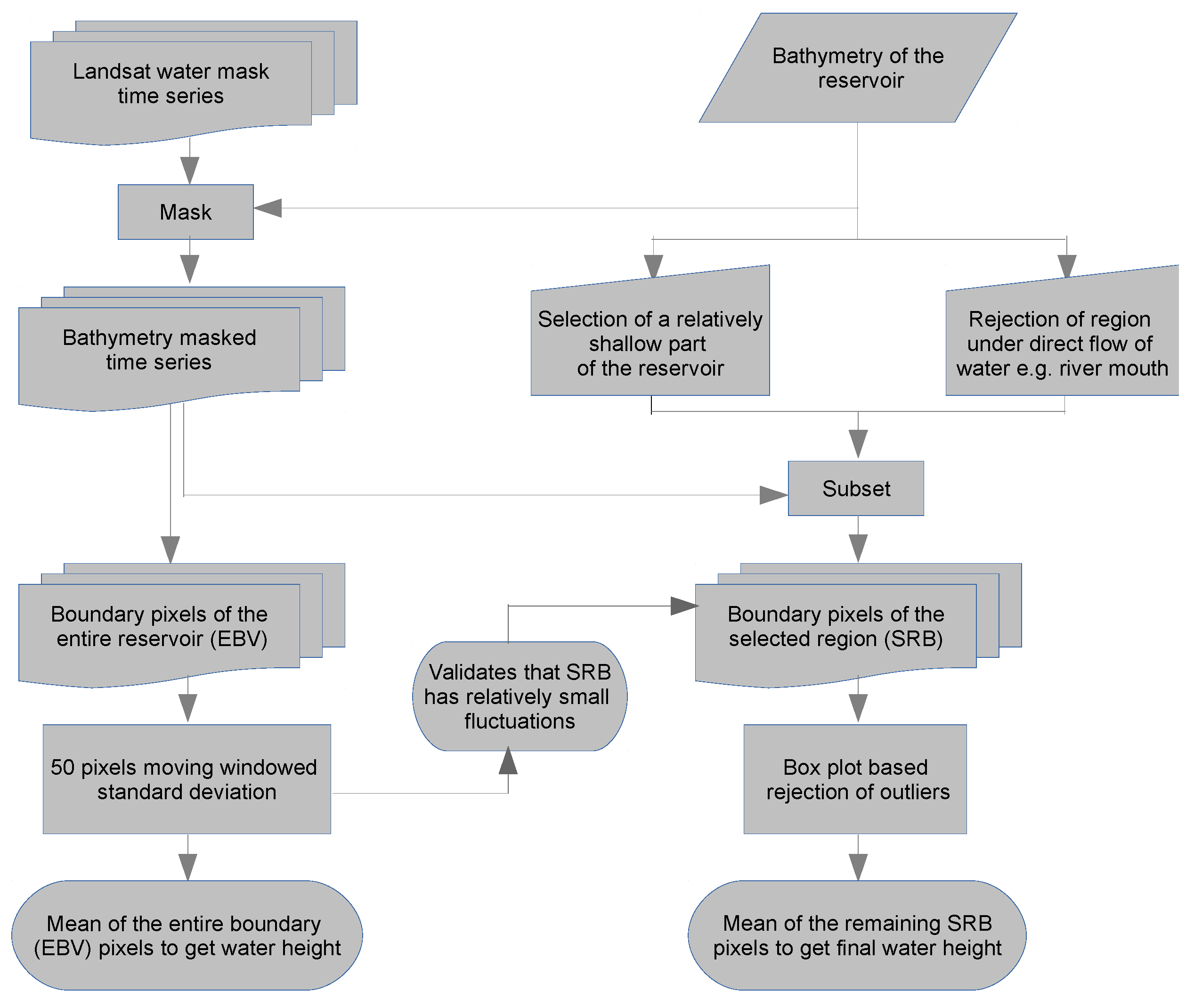
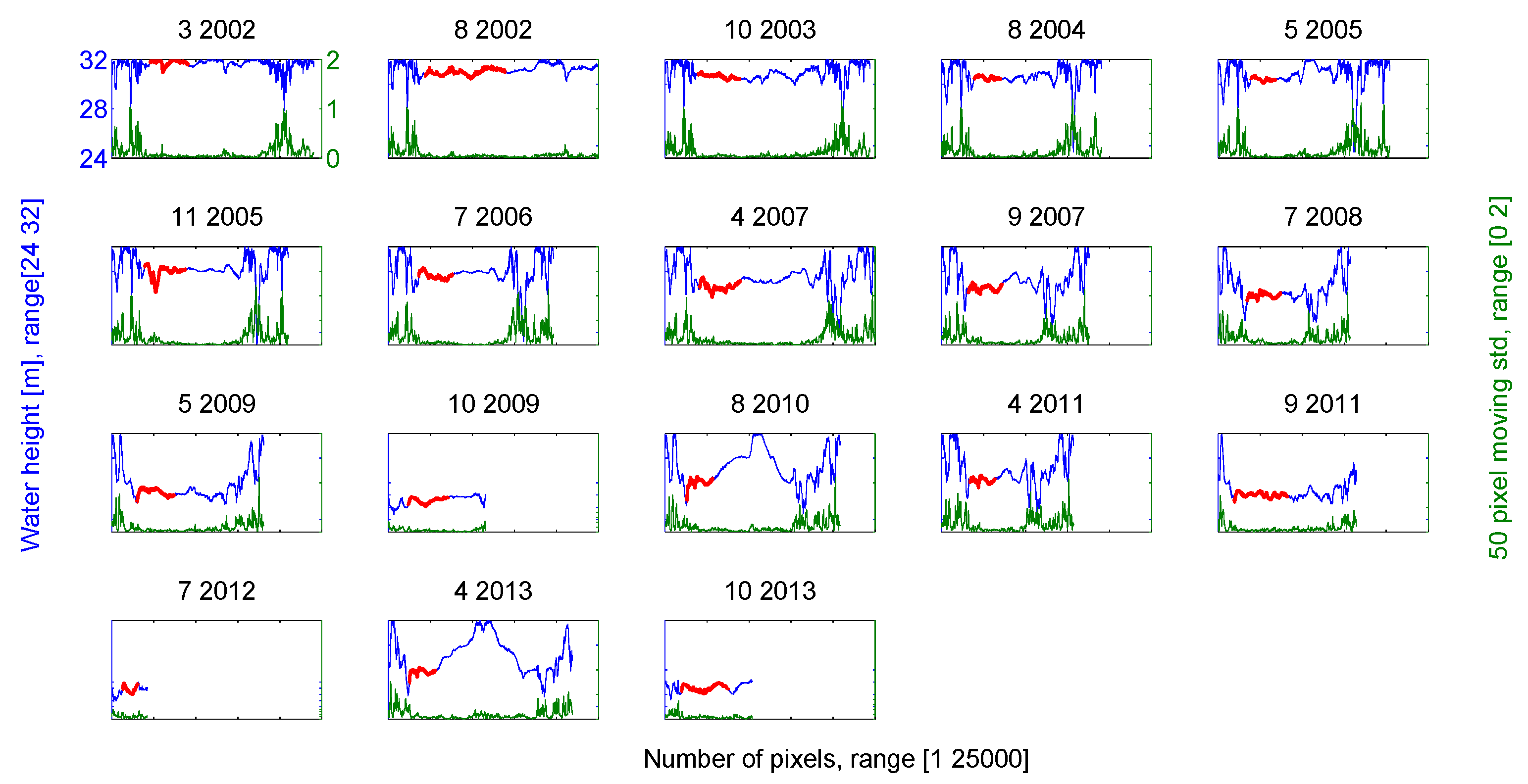
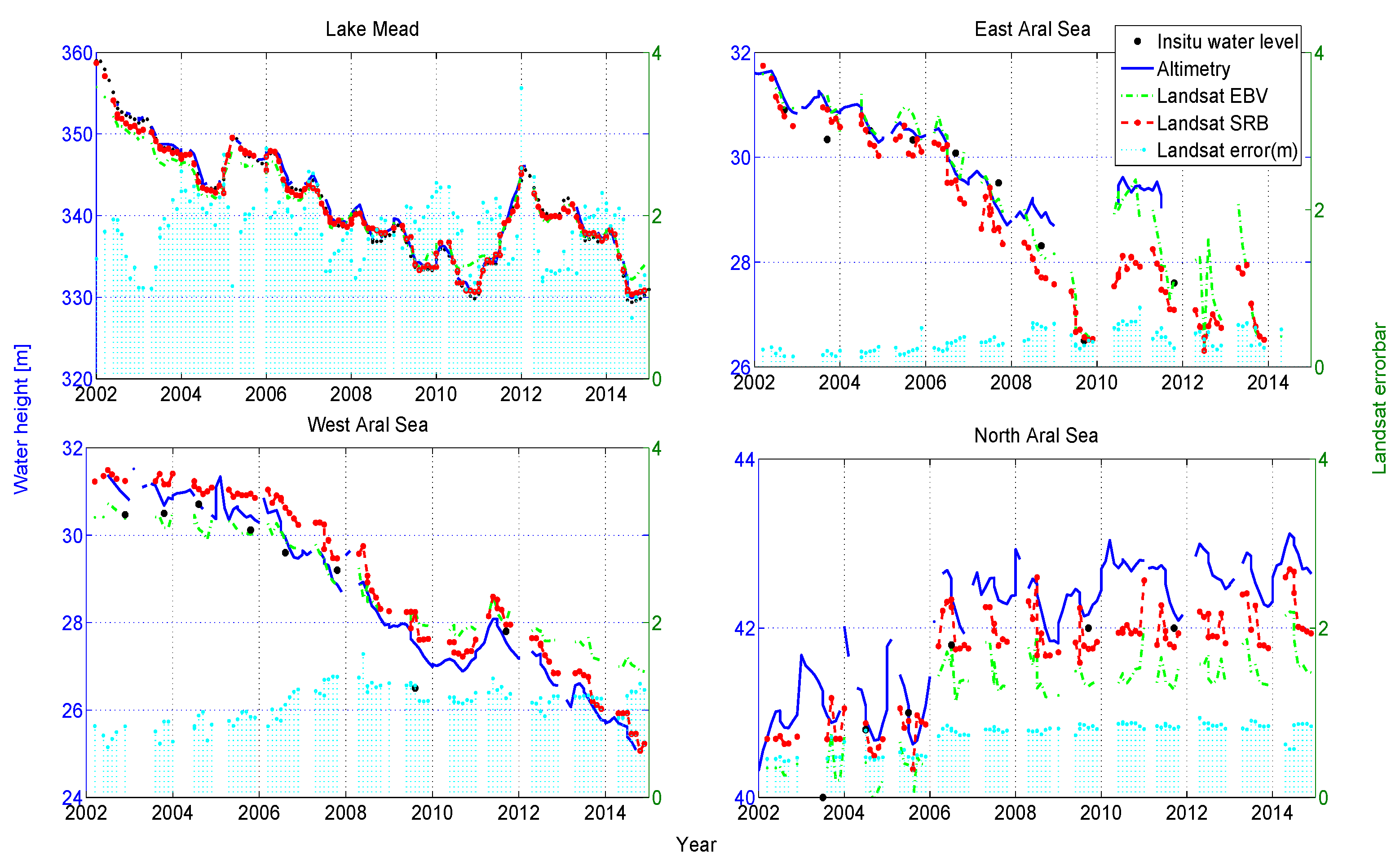
4.1. Water Height

4.2. Volumetric Variation

4.3. SSM Estimation and Prediction
4.3.1. Standard Case of Lake Mead


Filling up the Missing Data with SSM
| Reservoir | Compared Results | RMSE (NRMSE) | R2 | |
|---|---|---|---|---|
| Lake Mead | Landsat-SRB water height | In situ water height | 0.59 m (0.2%) | 0.99 |
| Altimetry water height | In situ water height | 0.67 m (0.2%) | 0.99 | |
| Landsat bathymetry volume (LBV) | In situ absolute volume | 0.32 km3 (1.6%) | 0.98 | |
| Altimetry bathymetry volume (ABV) | In situ absolute volume | 0.41 km3 (2.1%) | 0.97 | |
| Altimetry Landsat volume variation (ALVV) | In situ reduced by first obs. (volume variation) | 0.53 km3 | 0.96 | |
| ALVV | LBV reduced by first obs. | 0.31 km3 | 0.98 | |
| ALVV | ABV reduced by first obs. | 0.06 km3 | 0.99 | |
| Combined SSM estimate (CSSME) | In situ absolute volume | 0.35 km3 (1.8%) | 0.97 | |
| CSSME | LBV | 0.32 km3 (1.6%) | 0.98 | |
| CSSME | ABV | 0.41 km3 (2.1%) | 0.97 | |
| CSSME Forecast | CSSME | 0.53 km3 (3.0%) | 0.80 | |
| CSSME Forecast | In situ absolute volume | 0.66 km3 (3.7%) | 0.75 | |
| West Aral Sea | Landsat-SRB water height | Altimetry water height | 0.44 m (1.5%) | 0.94 |
| LBV | ABV | 1.58 km3 (4.5%) | 0.94 | |
| ALVV | LBV reduced by first obs. | 1.73 km3 | 0.94 | |
| ALVV | ABV reduced by first obs. | 1.09 km3 | 0.97 | |
| CSSME | LBV | 1.00 km3 (2.7%) | 0.97 | |
| CSSME | ABV | 0.50 km3 (1.6%) | 0.99 | |
| CSSME Forecast | CSSME | 0.52 km3 (1.9%) | 0.76 | |
| North Aral Sea | Landsat-SRB water height | Altimetry water height | 0.50 m (1.2%) | 0.32 |
| LBV | ABV | 1.59 km3 (6.0%) | 0.23 | |
| ALVV | LBV reduced by first obs. | 1.46 km3 | 0.56 | |
| ALVV | ABV reduced by first obs. | 0.15 km3 | 0.99 | |
| CSSME | LBV | 0.82 km3 (3.2%) | 0.83 | |
| CSSME | ABV | 0.82 km3 (3.1%) | 0.83 | |
| CSSME Forecast | CSSME | 1.09 km3 (3.9%) | 0.23 | |
| East Aral Sea | Landsat-SRB water height (January 2002–December 2007) | Altimetry water height | 0.33 m (1.0%) | 0.82 |
| LBV (01.2002–12.2007) | ABV (January 2002–December 2007) | 2.40 km3 (13%) | 0.85 | |
| ALVV | LBV reduced by first obs. | 4.26 km3 | 0.51 | |
| ALVV | ABV reduced by first obs. | 0.67 km3 | 0.99 | |
| CSSME (January 2002–December 2007) | LBV (January 2002–December 2007) | 1.92 km3 (12.0%) | 0.89 | |
| CSSME (January 2002–December 2007) | ABV (January 2002–December 2007) | 0.49 km3 (2.7%) | 0.99 | |
| Entire Aral Sea | LBV | ABV | 4.10 km3 (5.5%) | 0.91 |
| CSSME Forecast | CSSME | 1.40 km3 (2.4%) | 0.60 | |
Combined SSM Estimate (CSSME) and Forecast
4.3.2. CSSME and Forecast for Aral Sea
4.4. Validation
4.4.1. Validation of Water Height
4.4.2. Validation of the Estimated Water Volume (LBV, ABV and ALVV)
4.4.3. Validation of CSSME Volume
4.5. Improved Bathymetry

5. Discussion
6. Conclusions
Acknowledgments
Author Contributions
Conflicts of Interes
References
- Feng, M.; Sexton, J.O.; Channan, S.; Townshend, J.R. A global, high-resolution (30-m) inland water body dataset for 2000: First results of a topographic-spectral classification algorithm. Int. J. Digit. Earth 2015. [Google Scholar] [CrossRef]
- Verpoorter, C.; Kutser, T.; Seekell, D.A.; Tranvik, L.J. A global inventory of lakes based on high-resolution satellite imagery. Geophys. Res. Lett. 2014, 41, 6396–6402. [Google Scholar] [CrossRef]
- Carroll, M.L.; Townshend, J.R.; DiMiceli, C.M.; Noojipady, P.; Sohlberg, R.A. A new global raster water mask at 250 m resolution. Int. J. Digit. Earth 2009, 2, 291–308. [Google Scholar] [CrossRef]
- Cretaux, J.-F.; Letolle, R.; Bergé-Nguyen, M. History of Aral Sea level variability and current scientific debates. Glob. Planet. Chang. 2013, 110, 99–113. [Google Scholar] [CrossRef]
- Schwatke, C.; Dettmering, D.; Bosch, W.; Seitz, F. DAHITI—An innovative approach for estimating water level time series over inland waters using multi-mission satellite altimetry. Hydrol. Earth Syst. Sci. 2015, 19, 4345–4364. [Google Scholar] [CrossRef]
- Asadzadeh Jarihani, A.; Callow, J.N.; Johansen, K.; Gouweleeuw, B. Evaluation of multiple satellite altimetry data for studying inland water bodies and river floods. J. Hydrol. 2013, 505, 78–90. [Google Scholar] [CrossRef]
- Forootan, E.; Rietbroek, R.; Kusche, J.; Sharifi, M.A.; Awange, J.L.; Schmidt, M.; Omondi, P.; Famiglietti, J. Separation of large scale water storage patterns over Iran using GRACE, altimetry and hydrological data. Remote Sens. Environ. 2014, 140, 580–595. [Google Scholar] [CrossRef]
- Wulder, M.A.; White, J.C.; Masek, J.G.; Dwyer, J.; Roy, D.P. Continuity of Landsat observations: Short term considerations. Remote Sens. Environ. 2011, 115, 747–751. [Google Scholar] [CrossRef]
- Bhagat, V.S.; Sonawane, K.R. Use of Landsat ETM+ data for delineation of water bodies in hilly zones. J. Hydroinform. 2011, 13, 661–671. [Google Scholar] [CrossRef]
- Rokni, K.; Ahmad, A.; Selamat, A.; Hazini, S. Water feature extraction and change detection using multitemporal Landsat imagery. Remote Sens. 2014, 6, 4173–4189. [Google Scholar] [CrossRef]
- Goward, S.N.; Williams, D.L. Landsat and earth systems science: Development of terrestrial monitoring. Photogramm. Eng. Remote Sens. 1997, 63, 887–900. [Google Scholar]
- Cretaux, J.-F.; Kouraev, A.; Berge-Nguyen, M.; Cazenave, A.; Papa, F. Satellite altimetry for monitoring lake level changes. In Transboundary Water Resources: Strategies for Regional Security and Ecological Stability; Vogtmann, H., Dobretsov, N., Eds.; NATO Science Series; Springer Netherlands: Novosibirsk, Russia, 2005; pp. 141–146. [Google Scholar]
- Medina, C.; Gomez-Enri, J.; Alonso, J.J.; Villares, P. Water volume variations in Lake Izabal (Guatemala) from in situ measurements and ENVISAT Radar Altimeter (RA-2) and Advanced Synthetic Aperture Radar (ASAR) data products. J. Hydrol. 2010, 382, 34–48. [Google Scholar] [CrossRef]
- Andreoli, R.; Li, J.; Yesou, H. Flood extent prediction from lake heights and water level estimation from flood extents using river gauges, elevation models and ENVISAT data. In Proceedings of the ENVISAT Symposium 2007, Montreux, Switzerland, 23–27 April 2007.
- Smith, L.C.; Pavelsky, T.M. Remote sensing of volumetric storage changes in lakes. Earth Surf. Process. Landf. 2009, 34, 1353–1358. [Google Scholar] [CrossRef]
- Baup, F.; Frappart, F.; Maubant, J. Combining high-resolution satellite images and altimetry to estimate the volume of small lakes. Hydrol. Earth Syst. Sci. 2014, 18, 2007–2020. [Google Scholar] [CrossRef]
- Duan, Z.; Bastiaanssen, W.G.M. Estimating water volume variations in lakes and reservoirs from four operational satellite altimetry databases and satellite imagery data. Remote Sens. Environ. 2013, 134, 403–416. [Google Scholar] [CrossRef]
- Abileah, R.; Vignudelli, S.; Scozzari, A. A completely remote sensing approach to monitoring reservoirs water volume. Int. Water Technol. J. 2011, 1, 59–72. [Google Scholar]
- Gao, H.; Birkett, C.; Lettenmaier, D.P. Global monitoring of large reservoir storage from satellite remote sensing. Water Resour. Res. 2012, 48, W09504. [Google Scholar] [CrossRef]
- Gao, H. Satellite remote sensing of large lakes and reservoirs: From elevation and area to storage. Wiley Interdiscip. Rev. Water 2015, 2, 147–157. [Google Scholar] [CrossRef]
- Bae, K.; Harris, D. A comparison of state space and multiple regression for monthly forecasts: U.S. Fuel consumption. Nonrenew. Resour. 1995, 4, 325–339. [Google Scholar] [CrossRef]
- Pao, H.-T. Forecast of electricity consumption and economic growth in Taiwan by state space modeling. Energy 2009, 34, 1779–1791. [Google Scholar] [CrossRef]
- Kumar, P. A multiple scale state-space model for characterizing subgrid scale variability of near-surface soil moisture. IEEE Trans. Geosci. Remote Sens. 1999, 37, 182–197. [Google Scholar] [CrossRef]
- Ramos, P.; Santos, N.; Rebelo, R. Performance of state space and ARIMA models for consumer retail sales forecasting. Robot. Comput.-Integr. Manuf. 2015, 34, 151–163. [Google Scholar] [CrossRef]
- Wallerman, J.; Vencatasawmy, C.P.; Bondesson, L. Spatial simulation of forest using Bayesian state-space models and remotely sensed data. In Proceedings of the 7th International Symposium on Spatial Accuracy Assessment in Natural Resources and Environmental Sciences, Lisbon, Portugal, 5–7 July 2006.
- Zavialov, P.O. Physical Oceanography of the Dying Aral Sea; Springer Science & Business Media: Heidelberg, Germany, 2005. [Google Scholar]
- Micklin, P. Aral sea basin water resources and the changing aral water balance. In The Aral Sea; Micklin, P., Aladin, N.V., Plotnikov, I., Eds.; Springer Earth System Sciences; Springer: Berlin, Germany; Heidelberg, Germany, 2014; pp. 111–135. [Google Scholar]
- UN Documentation Centre on Water and Sanitation (UNDCWS). Available online: http://www.zaragoza.es/ciudad/medioambiente/onu/en/detallePer_Onu?id=866 (accessed on 1 October 2014).
- Pat, S.; Esad, M.; Gyanesh, C. SLC Gap-Filled Products Phase One Methodology. Available online: http://landsat.usgs.gov 2004 (accessed on 2 October 2015).
- Benduhn, F.; Renard, P. A dynamic model of the Aral Sea water and salt balance. J. Mar. Syst. 2004, 47, 35–50. [Google Scholar] [CrossRef]
- Singh, A.; Seitz, F.; Schwatke, C. Application of Multi-sensor satellite data to observe water storage variations. IEEE J. Sel. Top. Appl. Earth Obs. Remote Sens. 2013, 6, 1502–1508. [Google Scholar] [CrossRef]
- USGS. USGS Open-File Report 03-320 Mapping the Floor of Lake Mead (Nevada and Arizona): Preliminary Discussion and GIS Data Release, Metadata and Data. Available online: http://pubs.usgs.gov/of/2003/of03-320/htmldocs/datacatalog.htm#surfacesutm (accessed on 16 November 2015).
- Hubert, M.; Vandervieren, E. An adjusted boxplot for skewed distributions. Comput. Stat. Data Anal. 2008, 52, 5186–5201. [Google Scholar] [CrossRef]
- Kitanidis, P.K. Introduction to Geostatistics: Applications to Hydrogeology; Cambridge University Press: Cambridge, UK; New York, NY, USA, 1997. [Google Scholar]
- Sawitzki, G. Computational Statistics: An Introduction to R; CRC Press: Boca Raton, FL, USA, 2009. [Google Scholar]
- Durbin, J.; Koopman, S.J. Time Series Analysis by State Space Methods, 2nd ed.; Oxford University Press: Oxford, UK, 2012. [Google Scholar]
- Shumway, R.H.; Stoffer, D.S. Time Series Analysis and Its Applications: With R Examples, 3rd ed.; Springer: New York, NY, USA, 2011. [Google Scholar]
- Singh, A.; Seitz, F.; Schwatke, C. Inter-annual water storage changes in the Aral Sea from multi-mission satellite altimetry, optical remote sensing, and GRACE satellite gravimetry. Remote Sens. Environ. 2012, 123, 187–195. [Google Scholar] [CrossRef]
- Birkett, C.; Reynolds, C.; Beckley, B.; Doorn, B. From research to operations: The USDA global reservoir and lake monitor. In Coastal Altimetry; Vignudelli, S., Kostianoy, A.G., Cipollini, P., Benveniste, J., Eds.; Springer: Berlin, Germany; Heidelberg, Germany, 2011; pp. 19–50. [Google Scholar]
- Singh, A.; Seitz, F. Updated Bathymetric Chart of the East Aral Sea; Data Publisher for Earth & Environmental Science: Bremerhaven, Germany, 2015. [Google Scholar] [CrossRef]
- Ablain, M.; Cazenave, A.; Valladeau, G.; Guinehut, S. A new assessment of the error budget of global mean sea level rate estimated by satellite altimetry over 1993-2008. Ocean Sci. 2009, 5, 193–201. [Google Scholar] [CrossRef]
© 2015 by the authors; licensee MDPI, Basel, Switzerland. This article is an open access article distributed under the terms and conditions of the Creative Commons by Attribution (CC-BY) license (http://creativecommons.org/licenses/by/4.0/).
Share and Cite
Singh, A.; Kumar, U.; Seitz, F. Remote Sensing of Storage Fluctuations of Poorly Gauged Reservoirs and State Space Model (SSM)-Based Estimation. Remote Sens. 2015, 7, 17113-17134. https://doi.org/10.3390/rs71215872
Singh A, Kumar U, Seitz F. Remote Sensing of Storage Fluctuations of Poorly Gauged Reservoirs and State Space Model (SSM)-Based Estimation. Remote Sensing. 2015; 7(12):17113-17134. https://doi.org/10.3390/rs71215872
Chicago/Turabian StyleSingh, Alka, Ujjwal Kumar, and Florian Seitz. 2015. "Remote Sensing of Storage Fluctuations of Poorly Gauged Reservoirs and State Space Model (SSM)-Based Estimation" Remote Sensing 7, no. 12: 17113-17134. https://doi.org/10.3390/rs71215872