
Using Stochastic Ray Tracing to Simulate a Dense Time Series of Gross Primary Productivity


Abstract
:
1. Introduction
2. Methods
2.1. Study Area
2.2. Data
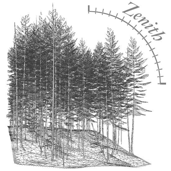
2.3. Scene Reconstruction


2.4. Canopy Radiation Modeling
2.5. Photosynthesis Modeling
2.6. Model Inversion


| Case | Enabled Modifier Functions | Fixed Parameters | Free Parameters |
|---|---|---|---|
| 1 | None | ||
| 2 | |||
| 3 | |||
| 4 |
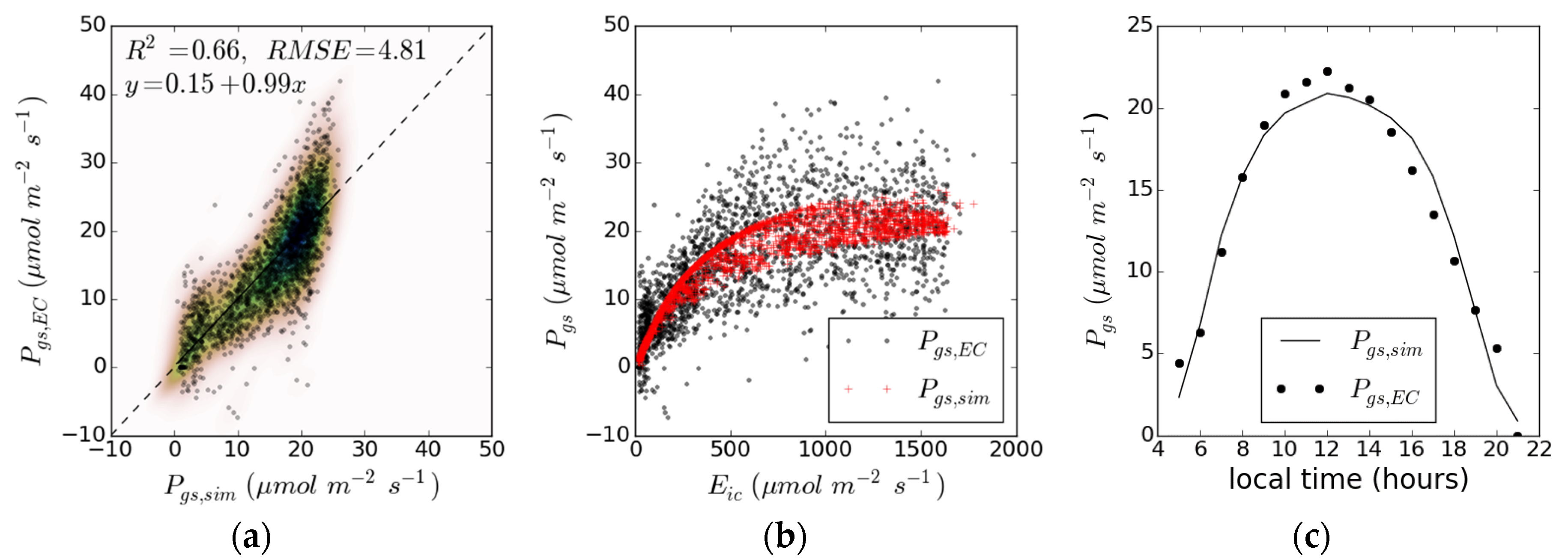
3. Results


| Case | |||||||||||
|---|---|---|---|---|---|---|---|---|---|---|---|
| 10 | 1 | 8.545 | 0.089 | - | - | - | - | - | - | - | - |
| 2 | 10.896 | 0.097 | 19.554 | - | 112.424 | 24.251 | - | 0.632 | 0.121 | - | |
| 3 | 12.481 | 0.104 | 19.554 | 1005.216 | 103.788 | 24.251 | 1710.711 | 0.694 | 0.121 | - | |
| 4 | 65.984 | 0.153 | 19.554 | 994.088 | 103.788 | 24.251 | 1700.244 | 0.694 | 0.121 | 0.411 | |
| 15 | 1 | 8.546 | 0.089 | - | - | - | - | - | - | - | - |
| 2 | 10.896 | 0.097 | 19.544 | - | 112.485 | 24.242 | - | 0.632 | 0.121 | - | |
| 3 | 12.480 | 0.104 | 19.544 | 1005.115 | 103.826 | 24.242 | 1710.440 | 0.694 | 0.121 | - | |
| 4 | 65.524 | 0.153 | 19.544 | 993.867 | 103.826 | 24.242 | 1700.426 | 0.694 | 0.121 | 0.409 | |
| 20 | 1 | 8.544 | 0.089 | - | - | - | - | - | - | - | - |
| 2 | 10.892 | 0.097 | 19.542 | - | 112.495 | 24.231 | - | 0.633 | 0.121 | - | |
| 3 | 12.478 | 0.104 | 19.542 | 1004.874 | 103.832 | 24.231 | 1710.720 | 0.694 | 0.121 | - | |
| 4 | 64.873 | 0.152 | 19.542 | 993.612 | 103.832 | 24.231 | 1701.675 | 0.694 | 0.121 | 0.406 |

4. Discussion
5. Conclusions
Acknowledgments
Author Contributions
Conflicts of Interest
List of Symbols
| Symbol | Units * | Description |
|---|---|---|
| μmol·C·μmol-1·photons | quantum yield | |
| μmol·C·μmol-1·photons | theoretical optimum for quantum yield | |
| % | sensitivity of to changes in | |
| °C·days | sensitivity of to changes in | |
| μmol·photons·m-2·s-1 | sensitivity of to changes in | |
| °C | sensitivity of to changes in | |
| lag in response of to changes in | ||
| lag in response of to changes in | ||
| radians | zenith angle | |
| vector of model parameters | ||
| reflectance | ||
| collided and un-collided transmittance, respectively | ||
| radians | azimuth angle | |
| duration of initial linear response for eq. 2 | ||
| steradians | solid angle; | |
| steradians | projected solid angle; | |
| m2 | area of facet (solid portion for porous facets) | |
| m2 | area of reference plane | |
| °C·days | growing degree days | |
| modifier | ||
| °C·days | optimal growing degree day for photosynthesis | |
| μmol·photons·m-2·s-1 | photosynthetically active radiation (irradiance) | |
| μmol·photons·m-2·s-1 | incident on the canopy | |
| μmol·photons·m-2·s-1 | absorbed by the canopy | |
| μmol·photons·m-2·s-1 | absorbed by a canopy element | |
| modifier | ||
| % | relative humidity | |
| modifier | ||
| exponential N-allocation coefficient | ||
| μmol·photons·m-2·s-1·sr-1 | radiance | |
| μmol·photons·m-2·s-1·sr-1 | radiance at reference plane above canopy | |
| absorption probability | ||
| μmol·C·m-2·s-1 | gross primary productivity | |
| μmol·C·m-2·s-1 | at stand level | |
| μmol·C·m-2·s-1 | at canopy element level | |
| μmol·C·m-2·s-1 | photosynthetic capacity at leaf () level | |
| μmol·C·m-2·s-1 | optimal photosynthetic capacity at leaf () level | |
| scene element (i.e., facet) | ||
| ,, | foliage, soil, and bark elements, respectively | |
| °C | air temperature | |
| modifier | ||
| °C | optimal temperature for photosynthesis |
References
- Coops, N.C.; Wulder, M.A.; Duro, D.C.; Han, T.; Berry, S. The development of a Canadian dynamic habitat index using multi-temporal satellite estimates of canopy light absorbance. Ecol. Indic. 2008, 8, 754–766. [Google Scholar] [CrossRef]
- Kurz, W.A.; Dymond, C.C.; Stinson, G.; Rampley, G.J.; Neilson, E.T.; Carroll, A.L.; Ebata, T.; Safranyik, L. Moutain pine beetle and forest carbon feedback to climate change. Nature 2008, 452, 987–990. [Google Scholar] [CrossRef] [PubMed]
- Monteith, J.L. Solar radiation and productivity in tropical ecosystems. J. Appl. Ecol. 1972, 9, 747–766. [Google Scholar] [CrossRef]
- Monteith, J.L. Climate and the efficiency of crop production in Britain. Philos. Trans. R. Soc. Lond. Ser. B Biol. Sci. 1977, 281, 277–294. [Google Scholar] [CrossRef]
- Wang, Y.-P.; Jarvis, P.G. Description and validation of an array model—MAESTRO. Agric. For. Meteorol. 1990, 51, 257–280. [Google Scholar] [CrossRef]
- Heinsch, F.A.; Reeves, M.; Votava, P.; Kang, S.; Milesi, C.; Glassy, J.; Jolly, W.M.; Loehman, R.; Bowker, C.F.; Kimball, J.S.; et al. User’s Guide GPP and NPP (MOD17A2/A3) Products NASA MODIS Land Algorithm. 2003. Available online: https://www.researchgate.net/publication/242118371_User's_Guide_GPP_and_NPP_MOD17A2A3_Products_NASA_MODIS_Land_Algorithm (accessed on 14 December 2015).
- Norman, J.M. Modeling the complete crop canopy. In Modification of the Aerial Environment of Plants; Barfield, B.J., Gerber, J.F., Eds.; American Society of Agricultural Engineers: St. Joseph, MI, USA, 1979; pp. 249–277. [Google Scholar]
- Yang, W.; Ni-Meister, W.; Kiang, N.Y.; Moorcroft, P.R.; Strahler, A.H.; Oliphant, A. A clumped-foliage canopy radiative transfer model for a global dynamic terrestrial ecosystem model II: Comparison to measurements. Agric. For. Meteorol. 2010, 150, 895–907. [Google Scholar] [CrossRef]
- Hall, F.G.; Hilker, T.; Coops, N.C. Data assimilation of photosynthetic light-use efficiency using multi-angular satellite data: I. Model formulation. Remote Sens. Environ. 2012, 121, 301–308. [Google Scholar] [CrossRef]
- Hilker, T.; Hall, F.G.; Tucker, C.J.; Coops, N.C.; Black, T.A.; Nichol, C.J.; Sellers, P.J.; Barr, A.; Hollinger, D.Y.; Munger, J.W. Data assimilation of photosynthetic light-use efficiency using multi-angular satellite data: II Model implementation and validation. Remote Sens. Environ. 2012, 121, 287–300. [Google Scholar] [CrossRef]
- Mäkelä, A.; Pulkkinen, M.; Kolari, P.; Lagergren, F.; Berbigier, P.; Lindroth, A.; Loustau, D.; Nikinmaa, E.; Vesala, T.; Hari, P. Developing an empirical model of stand GPP with the LUE approach: Analysis of eddy covariance data at five contrasting conifer sites in Europe. Glob. Chang. Biol. 2008, 14, 92–108. [Google Scholar] [CrossRef]
- Baldocchi, D.; Falge, E.; Gu, L.; Olson, R.; Hollinger, D.; Running, S.; Anthoni, P.; Bernhofer, C.; Davis, K.; Evans, R.; et al. FLUXNET: A new tool to study the temporal and spatial variability of ecosystem-scale carbon dioxide, water vapor, and energy flux densities. Bull. Am. Meteorol. Soc. 2001, 82, 2415–2434. [Google Scholar] [CrossRef]
- Baldocchi, D.D. Assessing the eddy covariance technique for evaluating carbon dioxide exchange rates of ecosystems: Past, present and future. Glob. Chang. Biol. 2003, 9, 479–492. [Google Scholar] [CrossRef]
- Liang, S. Quatitative Remote Sensing of Land Surfaces; John Wiley and Sons, Inc.: Hoboken, NJ, USA, 2004. [Google Scholar]
- Wang, Y.-P.; Jarvis, P.G. Influence of crown structural properties on PAR absorption, photosynthesis, and transpiration in Sitka spruce: Application of a model (MAESTRO). Tree Physiol. 1990, 7, 297–316. [Google Scholar] [CrossRef] [PubMed]
- Medlyn, B.E.; Dreyer, E.; Ellsworth, D.; Forstreuter, M.; Harley, P.C.; Kirschbaum, M.U.F.; Roux, X.L.E. Temperature response of parameters of a biochemically based model of photosynthesis. II. A review of experimental data. Plant Cell Environ. 2002, 25, 1167–1179. [Google Scholar] [CrossRef]
- Ibrom, A.; Jarvis, P.G.; Clement, R.; Morgenstern, K.; Oltchev, A.; Medlyn, B.E.; Wang, Y.P.; Wingate, L.; Moncrieff, J.B.; Gravenhorst, G. A comparative analysis of simulated and observed photosynthetic CO2 uptake in two coniferous forest canopies. Tree Physiol. 2006, 26, 845–864. [Google Scholar] [CrossRef] [PubMed]
- Disney, M.I.; Lewis, P.; North, P.R.J. Monte Carlo ray tracing in optical canopy reflectance modelling. Remote Sens. Rev. 2000, 18, 163–196. [Google Scholar] [CrossRef]
- Widlowski, J.-L. An overview of two decades of systematic evaluation of canopy radiative transfer models. Int. Arch. Photogramm. Remote Sens. Spat. Inf. Sci. 2010, XXXVIII(Part 7B), 648–653. [Google Scholar]
- Widlowski, J.-L.; Pinty, B.; Lopatka, M.; Atzberger, C.; Buzica, D.; Chelle, M.; Disney, M.; Gastellu-Etchegorry, J.-P.; Gerboles, M.; Gobron, N.; et al. The fourth radiation transfer model intercomparison (RAMI-IV): Proficiency testing of canopy reflectance models with ISO-13528. J. Geophys. Res. Atmos. 2013, 118, 6869–6890. [Google Scholar] [CrossRef]
- Alton, P.B.; North, P. Interpreting shallow, vertical nitrogen profiles in tree crowns: A three-dimensional, radiative-transfer simulation accounting for diffuse sunlight. Agric. For. Meteorol. 2007, 145, 110–124. [Google Scholar] [CrossRef]
- Prusinkiewicz, P.; Lindenmayer, A. The Algorithmic Beauty of Plants. 2004. Available online: http://algorithmicbotany.org/papers/abop/abop.pdf (accessed on 14 December 2015).
- Weber, J.; Penn, J. Creation and rendering of realistic trees. In SIGGRAPH 95; ACM: New York, NY, USA, 1995; pp. 119–128. [Google Scholar]
- Pradal, C.; Boudon, F.; Nouguier, C.; Chopard, J.; Godin, C. PlantGL: A Python-based geometric library for 3D plant modelling at different scales. Graph. Models 2009, 71, 1–21. [Google Scholar] [CrossRef] [Green Version]
- Huang, H.; Qin, W.; Liu, Q. RAPID: A radiosity applicable to porous individual objects for directional reflectance over complex vegetated scenes. Remote Sens. Environ. 2013, 132, 221–237. [Google Scholar] [CrossRef]
- Smolander, S.; Stenberg, P. A method to account for shoot scale clumping in coniferous canopy reflectance models. Remote Sens. Environ. 2003, 88, 363–373. [Google Scholar] [CrossRef]
- Aschoff, T.; Spiecker, H. Algorithms for the automatic detection of trees in laser scanner data. Int. Arch. Photogramm. Remote Sens. Spat. Inf. Sci. 2004, XXXVI(Part 8/W2), 71–75. [Google Scholar]
- Van Leeuwen, M.; Nieuwenhuis, M. Retrieval of forest structural parameters using LiDAR remote sensing. Eur. J. For. Res. 2010, 129, 749–770. [Google Scholar] [CrossRef]
- Bucksch, A.; Lindenbergh, R.; Menenti, M. SkelTre. Vis. Comput. 2010, 26, 1283–1300. [Google Scholar] [CrossRef]
- Côté, J.-F.; Widlowski, J.-L.; Fournier, R.A.; Verstraete, M.M. The structural and radiative consistency of three-dimensional tree reconstructions from terrestrial lidar. Remote Sens. Environ. 2009, 113, 1067–1081. [Google Scholar] [CrossRef]
- Raumonen, P.; Kaasalainen, M.; Åkerblom, M.; Kaasalainen, S.; Kaartinen, H.; Vastaranta, M.; Holopainen, M.; Disney, M.; Lewis, P. Fast automatic precision tree models from terrestrial laser scanner data. Remote Sens. 2013, 5, 491–520. [Google Scholar] [CrossRef]
- Van der Zande, D.; Stuckens, J.; Verstraeten, W.W.; Mereu, S.; Muys, B.; Coppin, P. 3D modeling of light interception in heterogeneous forest canopies using ground-based LiDAR data. Int. J. Appl. Earth Obs. Geoinf. 2011, 13, 792–800. [Google Scholar] [CrossRef]
- Van Leeuwen, M.; Coops, N.C.; Hilker, T.; Wulder, M.A.; Newnham, G.J.; Culvenor, D.S. Automated reconstruction of tree and canopy structure for modeling the internal canopy radiation regime. Remote Sens. Environ. 2013, 136, 286–300. [Google Scholar] [CrossRef]
- Amanatides, J.; Woo, A. A fast voxel traversal algorithm for ray tracing. In Proceedings of the European Computer Graphics Conference & Exhibition, Amsterdam, the Netherlands, 24–28 August 1987; pp. 1–10.
- Suffern, K. Ray Tracing from the Ground up; A.K. Peters/CRC Press: Wellesley, MA, USA, 2007. [Google Scholar]
- Coops, N.C.; Hilker, T.; Wulder, M.A.; St-Onge, B.; Newnham, G.J.; Siggins, A.; Trofymow, J.A. Estimating canopy structure of Douglas-fir forest stands from discrete-return LiDAR. Trees 2007, 21, 295–310. [Google Scholar] [CrossRef]
- Krishnan, P.; Black, T.A.; Jassal, R.S.; Chen, B.; Nesic, Z. Interannual variability of the carbon balance of three different-aged Douglas-fir stands in the Pacific Northwest. J. Geophys. Res. 2009, 114, G04011. [Google Scholar] [CrossRef]
- Morgenstern, K.; Black, T.A.; Humphreys, E.R.; Griffis, T.J.; Drewitt, G.B.; Cai, T.; Nesic, Z.; Spittlehouse, D.L.; Livingston, N.J. Sensitivity and uncertainty of the carbon balance of a Pacific Northwest Douglas-fir forest during an el Niño/la Niña cycle. Agric. For. Meteorol. 2004, 123, 201–219. [Google Scholar] [CrossRef]
- Hilker, T.; Hall, F.G.; Coops, N.C.; Lyapustin, A.; Wang, Y.; Nesic, Z.; Grant, N.; Black, T.A.; Wulder, M.A.; Kljun, N.; et al. Remote sensing of photosynthetic light-use efficiency across two forested biomes: Spatial scaling. Remote Sens. Environ. 2010, 114, 2863–2874. [Google Scholar] [CrossRef]
- Jassal, R.S.; Black, T.A.; Cai, T.; Ethier, G.; Pepin, S.; Brummer, C.; Nesic, Z.; Spittlehouse, D.L.; Trofymow, J.A. Impact of Nitrogen fertilization on carbon and water balances in a chronosequence of three Douglas-fir stands in the Pacific Northwest. Agric. For. Meteorol. 2010, 150, 208–218. [Google Scholar] [CrossRef]
- Chen, J.M.; Govind, A.; Sonnentag, O.; Zhang, Y.Q.; Barr, A.; Amiro, B. Leaf area index measurements at fluxnet-Canada forest sites. Agric. For. Meteorol. 2006, 140, 257–268. [Google Scholar] [CrossRef]
- Chen, B.; Black, A.; Coops, N.C.; Hilker, T.; Trofymow, T.; Morgenstern, K. Assessing tower flux footprint climatology and scaling between remotely sensed and eddy covariance measurements. Bound.-Layer Meteorol. 2009, 130, 137–167. [Google Scholar] [CrossRef]
- Hilker, T.; Coops, N.C.; Wulder, M.A.; Black, T.A.; Guy, R.D. The use of remote sensing in light use efficiency based models of gross primary production: A review of current status and future requirements. Sci. Total Environ. 2008, 404, 411–423. [Google Scholar] [CrossRef] [PubMed]
- Strahler, A.H.; Jupp, D.L.B.; Woodcock, C.E.; Schaaf, C.B.; Yao, T.; Zhao, F.; Yang, X.; Lovell, J.; Culvenor, D.; Newnham, G.; et al. Retrieval of forest structural parameters using a ground-based LiDAR instrument (Echidna®). Can. J. Remote Sens. 2008, 34, S426–S440. [Google Scholar] [CrossRef]
- Van Leeuwen, M.; Coops, N.C.; Wulder, M.A. Canopy surface reconstruction from a LiDAR point cloud using Hough transform. Remote Sens. Lett. 2010, 1, 125–132. [Google Scholar] [CrossRef]
- Liu, Y.; Yang, H.; Wang, W. Reconstructing B-spline curves from point clouds—A tangential flow approach using least squares minimization. In Proceedings of the IEEE International Conference on Shape Modeling and Applications 2005, Cambridge, MA, USA, 13–17 June2005; pp. 4–12.
- Nilson, T. A theoretical analysis of the frequency of gaps in plant stands. Agric. Meteorol. 1971, 8, 25–38. [Google Scholar] [CrossRef]
- Chen, J.M.; Black, T.A. Foliage area and architecture of plant canopies from sunfleck size distributions. Agric. For. Meteorol. 1992, 60, 249–266. [Google Scholar] [CrossRef]
- Jupp, D.L.B.; Culvenor, D.S.; Lovell, J.L.; Newnham, G.J.; Strahler, A.H.; Woodcock, C.E. Estimating forest LAI profiles and structural parameters using a ground-based laser called “Echidna”. Tree Physiol. 2009, 29, 171–181. [Google Scholar] [CrossRef] [PubMed]
- Schaepman-Strub, G.; Schaepman, M.E.; Painter, T.H.; Dangel, S.; Martonchik, J.V. Reflectance quantities in optical remote sensing—Definitions and case studies. Remote Sens. Environ. 2006, 103, 27–42. [Google Scholar] [CrossRef]
- Gastellu-Etchegorry, J.P.; Demarez, V.; Pinel, V.; Zagolski, F. Modeling radiative transfer in heterogeneous 3-D vegetation canopies. Remote Sens. Environ. 1996, 156, 131–156. [Google Scholar] [CrossRef]
- Cohen, M.F.; Wallace, J.R. Radiosity and Realistic Image Synthesis; Academic Press: London, UK, 1993. [Google Scholar]
- Piccini, D.; Littmann, A.; Nielles-Vallespin, S.; Zenge, M.O. Spiral phyllotaxis: the natural way to construct 3D radial trajectory in MRI. Magn. Reson. Med. 2011, 66, 1049–1056. [Google Scholar] [CrossRef] [PubMed]
- Vogel, H. A better way to construct the sunflower head. Math. Biosci. 1979, 44, 179–189. [Google Scholar] [CrossRef]
- Cannell, M.G.R.; Thornley, J.H.M. Temperature and CO2 responses of leaf and canopy photosynthesis: A clarification using the non-rectangular hyperbola model of photosynthesis. Ann. Bot. 1998, 82, 883–892. [Google Scholar] [CrossRef]
- Jarvis, A.J.; Stauch, V.J.; Schulz, K.; Young, P.C. The seasonal temperature dependency of photosynthesis and respiration in two deciduous forests. Glob. Chang. Biol. 2004, 10, 939–950. [Google Scholar] [CrossRef]
- Hirose, T.; Werger, M.J.A. Maximizing daily canopy photosyntheis with respect to the leaf nitrogen allocation pattern in the canopy. Oecologia 1987, 72, 520–526. [Google Scholar] [CrossRef]
- Jacquemoud, S.; Baret, F.; Andrieu, B.; Danson, F.M.; Jaggard, K. Extraction of vegetation biophysical parameters by inversion of the PROSPECT + SAIL models on sugar beet canopy reflectance data. Application to TM and AVIRIS sensors. Remote Sens. Environ. 1995, 52, 163–172. [Google Scholar] [CrossRef]
- Thornley, J.H.M. Instantaneous canopy photosynthesis: Analytical expressions for sun and shade leaves based on exponential ligth decay down the canopy and an acclimated non-rectangular hyperbola for leaf photosynthesis. Ann. Bot. 2002, 89, 451–458. [Google Scholar] [CrossRef] [PubMed]
- Wesely, M.L.; Hart, R.L. Variability of short term eddy-correlation estimates of mass exchange. In The Forest-Atmosphere Interaction; Hutchinson, B.A., Hicks, B.B., Reidel, D., Eds.; Springer: Dordrecht, The Netherlands, 1985; pp. 591–612. [Google Scholar]
- Chen, J.-L.; Reynolds, J.F.; Harley, P.C.; Tenhunen, J.D. Coordination theory of leaf nitrogen distribution in a canopy. Oecologia 1993, 93, 63–69. [Google Scholar] [CrossRef]
- Knohl, A.; Baldocchi, D.D. Effects of radiation on canopy gas exchange processes in a forest ecosystem. J. Geophys. Res. 2008, 113, G02023. [Google Scholar] [CrossRef]
- Cai, T.; Black, T.A.; Jassal, R.S.; Morgenstern, K.; Nesic, Z. Incorporating diffuse photosynthetically active radiation in a single-leaf model of canopy photosynthesis for a 56-year-old coastal Douglas-fir stand. Int. J. Biometeorol. 2009, 53, 135–148. [Google Scholar] [CrossRef] [PubMed]
- Wang, Y.-P.; Jarvis, P.G. Influence of shoot structure on the photosynthesis of Sitka spruce (Picea Sitchensis). Funct. Ecol. 1993, 7, 433–451. [Google Scholar] [CrossRef]
- Knyazikhin, Y.; Miessen, G.; Panfyorov, O.; Gravenhorst, G. Small-scale study of three-dimensional distribution of photosynthetically active radiation in a forest. Agric. For. Meteorol. 1997, 88, 215–239. [Google Scholar] [CrossRef]
- Jarvis, P.G. The interpretation of the variations in leaf water potential and stomatal conductance found in canopies in the field. Philos. Trans. R. Soc. B Biol. Sci. 1976, 273, 593–610. [Google Scholar] [CrossRef]
- Parker, G.G.; Harmon, M.E.; Lefsky, M.A.; Chen, J.; van Pelt, R.; Weis, S.B.; Thomas, S.C.; Winner, W.E.; Shaw, D.C.; Frankling, J.F. Three-dimensional structure of an Old-growth Pseudotsuga-Tsuga canopy and its implications for radiation balance, microclimate, and gas exchange. Ecosystems 2004, 7, 440–453. [Google Scholar] [CrossRef]
- Gamon, J.A.; Bond, B. Effects of irradiance and photosynthetic downregulation on the photochemical reflectance index in Douglas-fir and ponderosa pine. Remote Sens. Environ. 2013, 135, 141–149. [Google Scholar] [CrossRef]
- Hember, R.A.; Coops, N.C.; Black, T.A.; Guy, R.D. Simulating gross primary production across a chronosequence of coastal Douglas-fir forest stands with a production efficiency model. Agric. For. Meteorol. 2010, 150, 238–253. [Google Scholar] [CrossRef]
- Pearcy, R.W. Sunflecks and photosynthesis in plant canopies. Ann. Rev. Plant Physiol. Plant Mol. Biol. 1990, 41, 421–453. [Google Scholar] [CrossRef]
- Knyazikhin, Y.; Schull, M.A.; Stenberg, P.; Mottus, M.; Rautiainen, M.; Yang, Y.; Marshak, A.; Carmona, P.L.; Kaufmann, R.K.; Lewis, P.; et al. Hyperspectral remote sensing of foliar nitrogen content. Proc. Natl. Acad. Sci. USA 2013, 110, E185–E192. [Google Scholar] [CrossRef] [PubMed]
- Garrity, S.R.; Vierling, L.A.; Bickford, K. A simple filtered photodiode instrument for continuous measurement of narrowband NDVI and PRI over vegetated canopies. Agric. For. Meteorol. 2010, 150, 489–496. [Google Scholar] [CrossRef]
- Gamon, A.; Penuelas, J.; Field, C.B. A narrow-waveband spectral index that tracks diurnal changes in photosynthetic efficiency. Remote Sens. Lett. 1992, 41, 35–44. [Google Scholar] [CrossRef]
- Demmig-Adams, B.; Adams, W.W. Photoprotection in an ecological context: The remarkable complexity of thermal energy dissipation. New Phytol. 2006, 172, 11–21. [Google Scholar] [CrossRef] [PubMed]
© 2015 by the authors; licensee MDPI, Basel, Switzerland. This article is an open access article distributed under the terms and conditions of the Creative Commons by Attribution (CC-BY) license (http://creativecommons.org/licenses/by/4.0/).
Share and Cite
Van Leeuwen, M.; Coops, N.C.; Black, T.A. Using Stochastic Ray Tracing to Simulate a Dense Time Series of Gross Primary Productivity. Remote Sens. 2015, 7, 17272-17290. https://doi.org/10.3390/rs71215875
Van Leeuwen M, Coops NC, Black TA. Using Stochastic Ray Tracing to Simulate a Dense Time Series of Gross Primary Productivity. Remote Sensing. 2015; 7(12):17272-17290. https://doi.org/10.3390/rs71215875
Chicago/Turabian StyleVan Leeuwen, Martin, Nicholas C. Coops, and T. Andrew Black. 2015. "Using Stochastic Ray Tracing to Simulate a Dense Time Series of Gross Primary Productivity" Remote Sensing 7, no. 12: 17272-17290. https://doi.org/10.3390/rs71215875
APA StyleVan Leeuwen, M., Coops, N. C., & Black, T. A. (2015). Using Stochastic Ray Tracing to Simulate a Dense Time Series of Gross Primary Productivity. Remote Sensing, 7(12), 17272-17290. https://doi.org/10.3390/rs71215875