1. Introduction
The problem of ensuring food security for an increasing population is currently one of the main concerns globally. To solve economic and social issues resulting from current and predicted food shortage, one billion hectares of new cropland would be required in order to meet the demand for food by 2050 [
1]. However, taking into consideration environmental restrictions, the potential to expand cropland at the expense of other lands, such as forests or rangelands, is limited [
2]. The challenge for agronomists, farmers and their allied partners is to produce humanity’s food in an ecologically sustainable manner, through socially accepted production systems [
3]. These trends suggest an increasing demand for dependable and accurate agricultural monitoring to ensure sustainable crop production and investigation of land management practices [
4].
Within this framework, spatially explicit cropland information, such as cropland extent and crop type, is crucial to sustain agriculture and preserve natural resources. A basic prerequisite for the implementation of a land-management strategy is the development of up-to-date Land Use/Land Cover (LULC) databases over agricultural landscapes. Indeed, LULC data, regarding the spatial distribution of crop types, is considered as key information from a geostrategic point of view. The research community is moving towards providing and timely agricultural maps at national or global level of detail [
5].
Over the past decade satellite images offer a valuable source of information concerning the monitoring of the Earth’s surface in fine spectral and spatial scales. Satellite based earth observation has been used to map crop types under a variety of environmental conditions, providing synoptic coverage of fields in several spectral regions, smooth integration with existing geographical databases under a cost-effective and time-saving approach than traditional statistical surveys [
6]. Through these studies, remote sensing techniques have proven to be cost-effective in widespread agricultural lands in Africa, America, Europe and Australia.
Monitoring and mapping vegetation involves investigating vegetation dynamics, such as phenological states and the seasonal growth of crop types. Spectral behavior of agricultural parcels is constantly changing; different crop types may be at a certain instant in the same phenological state, depicting similar spectral attributes, but diverge remarkably in another instant. Classification of parcels based on single-date images, even if they are acquired at critical growth states, cannot offer reliable results in the case of crops with similar growing cycle. As a result, the significance of classification based on multi-temporal images has been well-recognized and especially regarding vegetation mapping, the usage of seasonal imagery is vital [
5,
7,
8,
9,
10,
11,
12].
Low resolution images with high revisit frequency have been processed on the continental and global scale, providing consistent information at high temporal resolution while covering large areas at low costs [
13]. However, because of sub-pixel heterogeneity, the spatial resolution of the imagery may result in significant errors in the estimated crop areas [
14,
15]
At the regional level, crop area estimations have been significantly improved since the introduction of the MODIS sensor with 250 meter ground resolution [
13]. MODIS offered unprecedented capabilities for large-area LULC mapping by providing global coverage, half-day revisit capacity and intermediate spatial resolution. Several studies have already demonstrated successfully the potential of these data for detailed LULC mapping in an agricultural setting [
15], especially for areas where the typical field size is large [
5,
16].
Multi-spectral, medium-high resolution images, acquired mainly by Landsat Thematic Mapper/Enhanced Thematic Mapper Plus (TM/ETM+), SPOT and RapidEye [
17,
18,
19,
20], have been used for regional to local scale crop mapping, either on mono-temporal basis or under a multi-temporal perspective, accounting for small sized fields or heterogeneous crop patterns. To solve the issue of high within-class variability originating from various agronomic practices, the synergy of multi-temporal optical and Synthetic Aperture Radar (SAR) data has also been proposed; the increased set of multi-temporal imagery enables the continuous monitoring of all stages of vegetation development [
21]. While multi-temporal data of medium-to-high resolution offers high potential for crop discrimination in fine-structured agricultural landscapes, integration of the temporal information in the classification process is not trivial. Precise annual mapping of crops, through an approach that could be used routinely over large areas, remains challenging [
22,
23].
Although a variety of algorithms has been employed in crop mapping studies, including among others, the minimum distance, Mahalanobis distance, maximum likelihood, spectral angle mapper and support vector machines, an approach integrating phenological models in the classification process has been given little attention so far. Through phenology, remote sensing observations and biophysical changes during vegetation’s growth can be linked statistically in order to discriminate crop types. A possible way of incorporating knowledge of phenology into the classification process lies on the adoption of the stochastic Hidden Markov Models (HMMs). HMMs allow the simulation of crop dynamics, exploiting the spectral information of their phenological states and their relations. In this regard, a common assumption is made that the vegetation signal and the different phenological states are considered random variables [
24]. The correlation of phenological states is described by different transition state probabilities in each crop model. As far as the different cultivation practices, the algorithm reckons the possibility of temporal variation in the phenological cycle. Different growing states of the same crop type per image can be introduced instead of using a generalized crop model. These states correspond to different spectral attributes and are used jointly to define each model. This is the basic advantage of HMMs compared to other techniques that produce simulations of average seasonal phenology [
25] and may fail to account for a restrained or accelerated phenological progress.
Previous work has tested the application of HMMs in Landsat time series to classify mountain vegetation in Norway [
26] and arable land in Brazil [
27], in MODIS-NDVI time series covering cultivated areas of the United States [
28] and NDVI data derived from the Advanced Very High Resolution Radiometer (AVHRR) over the West African savanna [
24]. In all the aforementioned studies, the low and medium resolution images have been reported to be adequate for the classification of large-sized agricultural holdings. However, Mediterranean regions that are characterized by distinct environmental and climate settings, high spatio-temporal ecological heterogeneity [
29,
30], variety of crop types and high fragmentation of farming lands [
23,
31], require a different approach.
The main aim of this study is the development of a robust crop mapping technique adopting the theory of Markov chains and phenological models, over a Euro-Mediterranean agricultural area. Specifically, this work proposes a crop classification approach that integrates high and medium resolution remote sensing images in order to monitor constant variations in the ecological process of the cropping systems. A pixel-based methodology was selected, instead of using the segment-based approach proposed by [
27], to avoid errors produced by segmentation algorithms. The per-segment approach applied to small-sized crop parcels, found over Euro-Mediterranean areas, may have the disadvantage of falsely including within field-crop objects small non-vegetated classes (
i.e., roads, canals) leading to an overestimation of the total vegetated area [
32].
In particular, the objectives of the study are: (1) the identification of different crop types using a sequence of four seasonal multispectral Landsat ETM+ and a RapidEye image, processed simultaneously through Hidden Markov Models, (2) the assessment of the impact on the accuracy of a pan-sharpening procedure applied to the lower resolution Landsat ETM+ imagery and (3) the investigation of the role of the temporal resolution and extent of the image sequence used, in relation to the phenological cycle of each crop type. The multi-sensor and multi- temporal approach is motivated by the acknowledgment of the potential of coarser spatial resolution data to cover large geographic extends, the demands of complex territories and the growing interest in exploiting multi-scale data synergistically [
4]. Furthermore, the definition of optimal temporal acquisition windows is considered vital by several crop mapping studies [
8,
11,
18,
33] while it can improve classification accuracy significantly.
2. Study Area
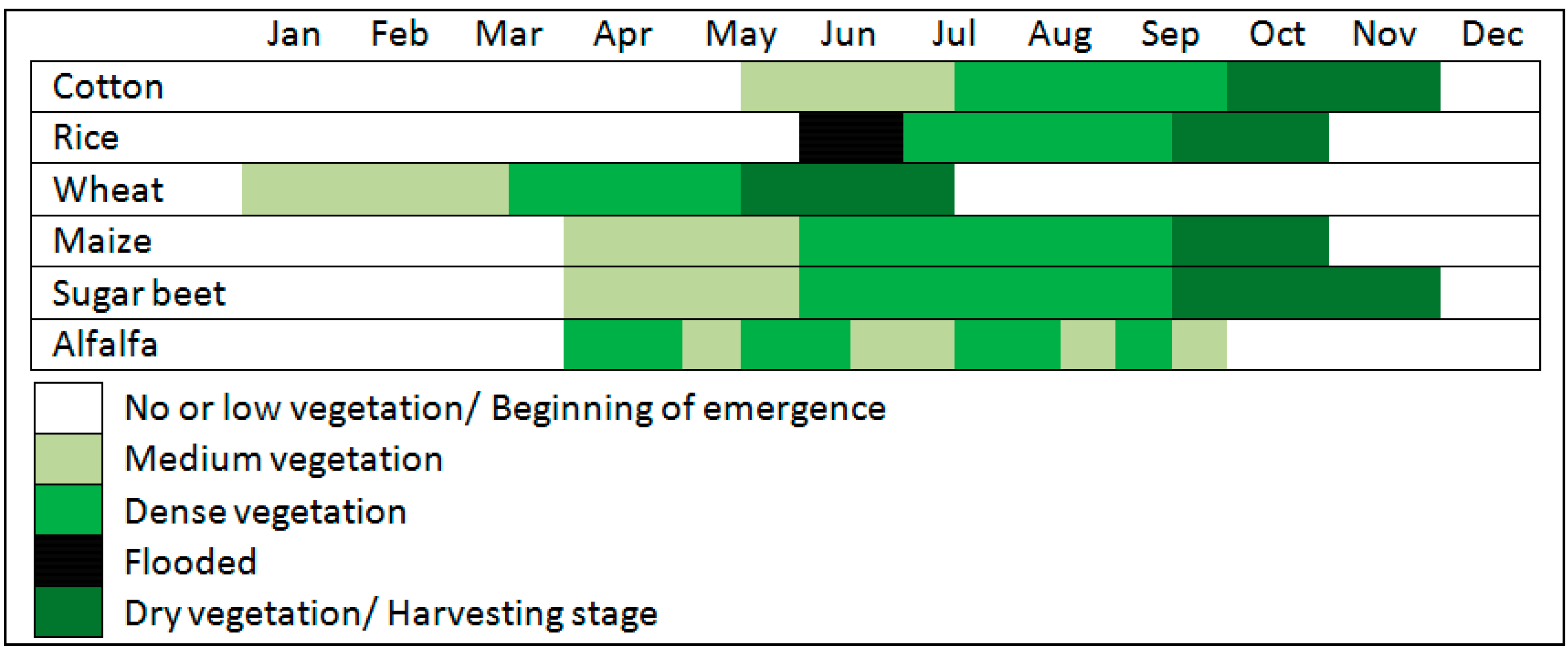
The research site is an irrigated agricultural area, near the city of Thessaloniki, Greece. The study area is dominated by rice and cotton while maize, sugar beet, wheat and alfalfa are planted to a smaller extent. The cropping calendar (planting and harvesting dates) of the area’s crop types is presented in
Figure 1.
Figure 1.
Idealized cropping calendar of the main crop types grown in the study area.
Figure 1.
Idealized cropping calendar of the main crop types grown in the study area.
Rice, cotton, maize and sugar beet are summer crops and those fields are characterized by dense vegetation during summer months. Wheat is harvested before June and is a spring crop. Rice, cotton, maize, sugar beet and wheat are considered annual crops and have a 12-months cycle. Alfalfa on the other hand can have 3–4 cuttings and flowerings per year, usually between May and September. Thus, the cropping pattern of the study area can be considered heterogeneous regarding the dates of planting, emergence, and harvesting. The majority of the parcels are rectangular but small sized. Despite the applied land consolidation the size of the parcels ranges from 0.006 to 10 ha. The terrain across the study area is relatively flat. The average annual temperature of the study area is 15.8 °C. The area is characterized by modest annual rainfall, averaging 441 mm/y.
3. Materials and Methods
3.1. Outline of the Methodology
Originally, the Landsat ETM+ images were registered to the higher resolution RapidEye image, which has been georeferenced using ground control points (GCPs) identified over VHR orthophotographs (
Figure 2) in the same geodetic system with the vector dataset representing field entities of the area (Land Parcel Identification System-LPIS). LPIS was visually corrected for small inconsistencies. The multispectral ETM+ images were pan-sharpened using the panchromatic band and the High Pass Filter (HPF) algorithm. Four synthetic images were produced with a spatial resolution of 15 meters. Nine different classifications experiments were applied on image sequences with variable spatial and temporal characteristics. A common set of training data, derived from the LPIS, was used to estimate the parameters of the crop models. For each HMM, we calculated the probability that the specific set of temporal observations corresponded to a class. Each pixel is assigned to the class whose crop-model emits the maximum probability. The results of the classification tests were evaluated in terms of overall accuracy and kappa coefficients.
Figure 2.
Overall process diagram of this research study.
Figure 2.
Overall process diagram of this research study.
3.2. Satellite Data and Preprocessing
Imagery acquired from sensors with different spectral, spatial and radiometric characteristics was used in the analysis. More specifically, the multispectral (excluding the thermal bands) and panchromatic components of four Landsat ETM+ images (184/32) and one multispectral RapidEye image, all acquired on different dates of 2010 (
Figure 3 and
Figure 4), were employed in this study (
Table 1).
Table 1.
Description of the satellite data used in the study. *: blue; G: green; R: red; NIR: near-infrared; SWIR: shortwave-infrared bands.
Table 1.
Description of the satellite data used in the study. *: blue; G: green; R: red; NIR: near-infrared; SWIR: shortwave-infrared bands.
Time
Step | Sensor | Date of Acquisition | Spatial Resolution Multi/Pan | Radiometric Resolution | Spectral Bands * |
|---|
| t1 | Landsat ETM+ | 07/05/2010 | 30/15 m | 8-bit | B, G, R, NIR, SWIR1, SWIR2 |
| t2 | Landsat ETM+ | 08/06/2010 | 30/15 m | 8-bit | B, G, R, NIR, SWIR1, SWIR2 |
| t3 | RapidEye | 05/08/2010 | 5 m | 16-bit | R, G, B, Red edge, NIR |
| t4 | Landsat ETM+ | 27/08/2010 | 30/15 m | 8-bit | B, G, R, NIR, SWIR1, SWIR2 |
| t5 | Landsat ETM+ | 30/10/2010 | 30/15 m | 8-bit | B, G, R, NIR, SWIR1, SWIR2 |
Landsat ETM + sensor launched in April 1999 has a spatial resolution of 30 meters for the six reflective bands, 60 meters for the thermal band, and 15 meters for the panchromatic (pan) band. On 31 May 2003, the ETM+ Scan Line Corrector (SLC) failed causing the scanning pattern to exhibit wedge‐shaped, scan-to-scan gaps, which are most pronounced along the edge of the scene. The scans give near-contiguous coverage of the surface scanned below the satellite in the center of the image (approximately 22 km wide).
RapidEye is a constellation of 5 multispectral satellite sensors launched in August 2008 with a primary focus on agricultural applications. The RapidEye sensor has a multispectral push broom imager with a spatial resolution of 6.25 meters. It captures data in five spectral bands covering visible–infrared part of the electromagnetic spectrum: blue (440–550 nm), green (520–590 nm), red (630–685 nm), red edge (690–730 nm), and near infrared (760–850 nm). In our study, we used the RapidEye (Level 3A) in which radiometric, sensor, and geometric correction have been applied and resampled to a 5 meters spatial resolution. We georeferenced the RapidEye imagery to the Greek Geodetic Reference System 1987, using ground control points, identified on natural color orthoimages with 50 cm spatial resolution acquired on 2007. Between 20 and 30 ground control points were used to co-register the Landsat scenes to the RapidEye imagery, with a Root Mean Square error (RMS) of less than a pixel. We did not apply any atmospheric correction or radiometric normalization since the adopted classification approach does not employ any direct comparison of pixel DN values between the temporal sequences of images. Instead, the classification scheme assigns pixels to crop classes, according to their similarity of states within each image separately and in a subsequent step the temporal images are linked using statistical relationships. In this context, atmospheric correction was not considered a prerequisite [
32].
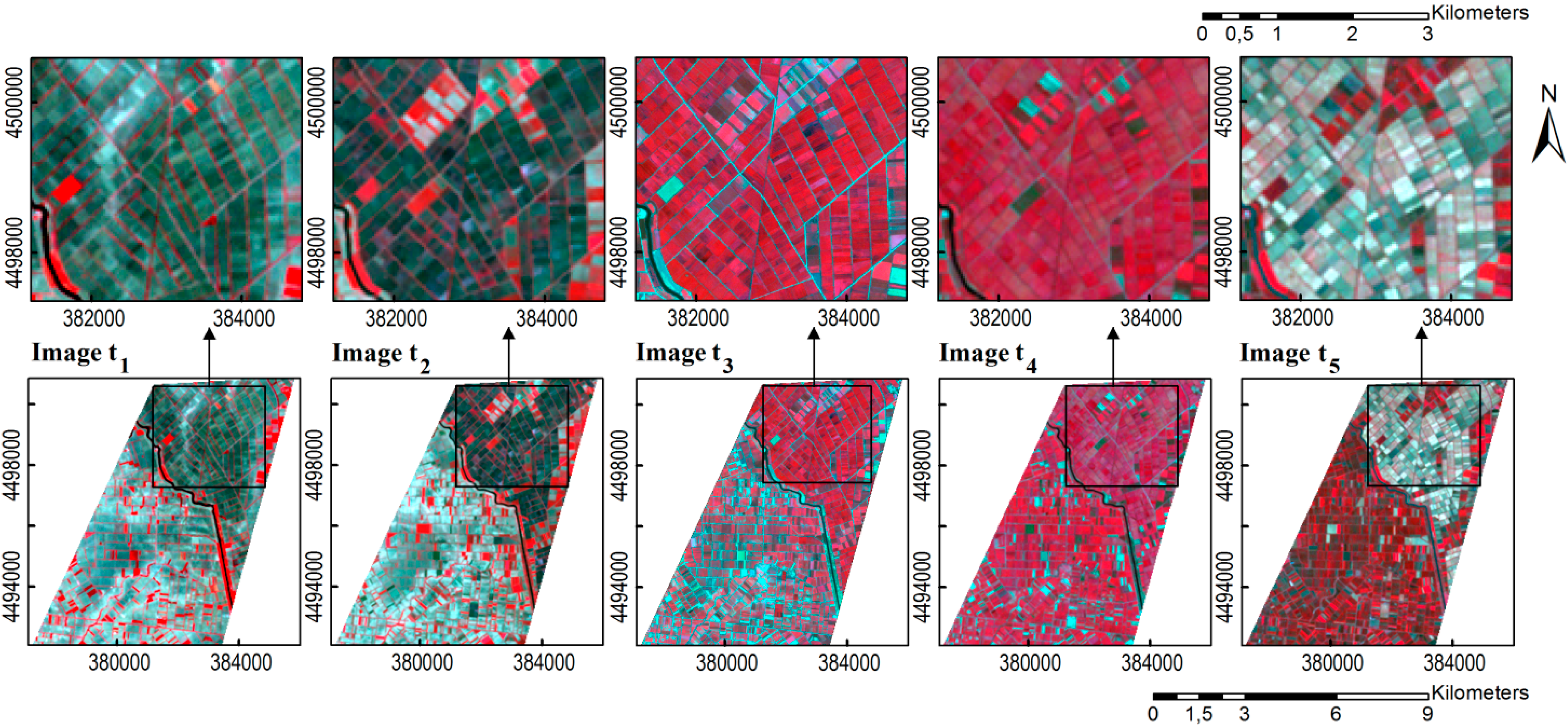
The same geographic subset was identified on every Landsat imagery, with no effective clouds or sensor defects, such as the “SLC-off problem”, covering approximately 7500 ha of cultivated area (1760 by 1710 RapidEye pixels). Additionally, regarding the Landsat images, the panchromatic images were merged with the multispectral ones, using the High Pass Filter (HPF) algorithm and four synthetic images were produced with a spatial resolution of 15 meters [
21]. Finally, in order to achieve spatial correspondence for each pixel, all Landsat ETM+ images (original and pan-sharpened) were re-sampled to 5 meters, using a nearest-neighbor algorithm to match the spatial resolution the RapidEye image (
Figure 3).
Figure 3.
The set of images used included four Landsat ETM+ images (image t1, image t2, image t4, image t5) illustrated in false-color composite (R: NIR, G:Red, B:Green) and one Rapideye image (image t3) in false-color composite (R: NIR, G:Red, B:Green).
Figure 3.
The set of images used included four Landsat ETM+ images (image t1, image t2, image t4, image t5) illustrated in false-color composite (R: NIR, G:Red, B:Green) and one Rapideye image (image t3) in false-color composite (R: NIR, G:Red, B:Green).
Figure 4.
The acquisition dates of the images used in the study.
Figure 4.
The acquisition dates of the images used in the study.
3.3. Reference Data
The Land Parcel Identification System (LPIS) is a fundamental part of the Integrated Administration and Control system that has been developed and adopted in 1992 by the EU as the spatial component for the implementation and supporting of the Common Agricultural Policy (CAP) and land management across Europe [
34]. The main functions of the LPIS are localization, identification and quantification of agricultural land via very detailed geospatial data, in order to spatially represent the activities of farmers on their land and facilitate the geographical identification of the agricultural parcels declared annually to receive funding [
35].
Although the regulatory requirements for the LPIS are uniform across the EU sector, the particular implementations are subject to member states. The Greek GIS-based LPIS integrates information about the crop type, the acreage of a parcel, the identity of the farmer and relates it to a vector layer comprised of the declared parcels. Since the information of this database is gathered from the declaration of the farmers it cannot be considered flawless. In this respect, an expert from “Greek Payment Authority of Common Agricultural Policy Aid Schemes of the Ministry of Rural Development and Food” visually examined and corrected the parcels’ crop type and boundaries manually, taking into account the cropping calendar of the study area and the spectral- temporal profile of each parcel. The detailed delineation of the boundaries was guided mainly by the high resolution RapidEye image. In total, 3319 declared parcels were found in the study area. A set of 55 parcels was used as training data and the rest was used during the accuracy assessment of the classification.
3.4. Description of the Proposed HMMs Classification Algorithm
The temporal evolution of vegetation can be described effectively by the state-oriented approach of Hidden Markov Models (HMMs). Each cultivated parcel has a dynamic behavior that depends on cropping phenology, climatic conditions, drought, water irrigation and chemical nutrients (
Figure 5).
Figure 5.
Temporal sequence of images t1, t2 and t3 covering the same area containing parcels cultivated by various crop types (1 = maize, 2 = rice, 3 = wheat, 4 = alfalfa and 5 = sugarcane). It is indicated that the different phenological states of crops at each time step impose significant variance in the between-class separability.
Figure 6.
Different subsets of satellite images t3 and t4 containing parcels with various crop types (1 = cotton, 2 = alfalfa and 3 = maize). In the left subset it can be observed that certain parcels of cotton and alfalfa may resemble according to their phenological state, while other parcels of the same crops can have distinct spectral properties. This can be also observed in the right subset referring to maize fields with different spectral characteristics.
Furthermore, neighboring parcels of the same crop type, over the same time step, may be at different states of growth due to varying agronomic practices; different planting or harvesting dates and fertilizers can accelerate or restrain the phenological progress (
Figure 6).
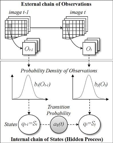
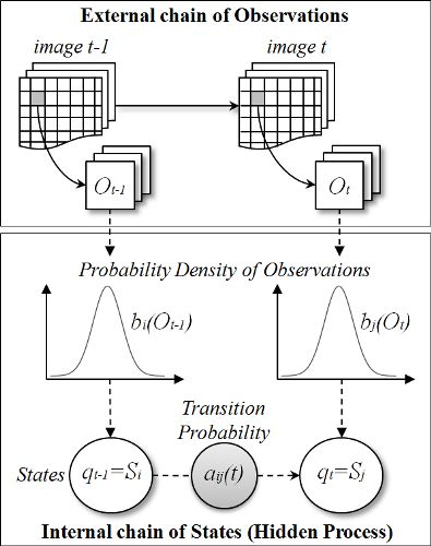
Given that each parcel changes constantly from state to state (
Figure 5) and that each state cannot be directly linked to a remote sensing measurement but to a probability distribution of observations, an HMM can be used to simulate the cycle of vegetation based on statistical relations. In this case, an HMM is a doubly embedded stochastic process comprised by two chains: the external chain of the remote sensing observations and the internal chain of states, which are unknown [
24] (
Figure 7).
Figure 7.
Schematic description of the basic elements of the proposed HMMs.
Figure 7.
Schematic description of the basic elements of the proposed HMMs.
In this study, a crop classification algorithm, based on Markov-chain analysis, was designed and implemented using Matlab®. Accordingly, a model was built describing the phenological states during the dates of the study for each crop type. The sequence of observations consisted of a set of remote sensing measurements O = {Ot1 ,..., Otn}, where t = {t1 ,..., tn} are the acquisition dates of the images. The hidden states correspond to the different phenological states S = {S1 ,..., Sm} of each crop type and Q = {qt1,..., qtn} is the fixed sequence of hidden states. During the acquisition of the satellite data, the identified states of the parcels in the study area were: S1, no vegetation or beginning of emergence, S2, medium vegetation or growth state, S3, dense vegetation or flowering and S4, dry vegetation or harvesting state.
An HMM is characterized by the following elements:
The state transition probability matrix A, where a
i,j(t) = P[q
t = S
j |q
t-1 = S
i], denotes the transition probability from state S
i to state S
j at time t. The emission probability matrix B, defines the probability that O
t is emitted by state S
j,
i.e., b
j(O
t) = P[O
t | q
t = S
j ]. In order to estimate the symbol probability distributions B, a multivariate Gaussian distribution is assumed for the observed spectral data. The mean vector
and the covariance matrix
were calculated by the training data for each crop type, for each state and for every image by the equation,
The initial probability π
i is the probability of being in state Si at time t1,
i.e., π
i = P[q
t1 = S
i]. The parameters A, B and π
i were estimated by the set of training data. The set of training samples was selected and defined according to our knowledge of local agronomic practices and the cropping calendar of the district. To ensure classification success, all classes need to be described by representative training samples. The samples define the different states of crop types according to their different spectral attributes. The set of the training data was evenly distributed in the study area, located in homogenous fields and not in boundary mixed pixels. It should also be noted that in each image, fields of the same crop type may be in different states; usually a state before or a state after (
Figure 6). Judging by the cropping calendar and the dates of the used images, not all transitions between states are possible in this case study. Once we have estimated the parameters A, B, π
i of each model λ and given the sequence of observations O for each pixel, the probability that the sequence O was generated by these models λ is defined by:
Detailed mathematical explanation of HMMs has been reported in previous studies [
24,
36] which propose the implementation of the Forward algorithm to simplify computations of Equation (2).
In this study, five models were built (one for each crop class), and five measurements of probability were estimated for each pixel (Equation (2)). Let us consider a temporal spectral sequence of pixel
x belonging to l
m, the most probable crop, where L = {l
1,..., l
k} is the set of possible crop classes. For each pixel
x, the most likely crop-class is determined by the following rule:
Finally, nine different HMM models were developed in order to evaluate the role of the temporal resolution and extent of the image sequence used, in relation to the phenological cycle of each crop type, as well as to assess the utility of the pan-sharpening procedure in terms of classification accuracy (
Table 2).
Table 2.
Selections of different images included in the evaluation of our proposed methodology.
Table 2.
Selections of different images included in the evaluation of our proposed methodology.
| | Imagery Employed | Rationale of the Classification Experiment |
|---|
| | t1 | t2 | t4 | t5 | t1 | t2 | t4 | t5 | t3 |
|---|
| Original ETM+ | Pan-Sharpened ETM+ | RapidEye |
|---|
| HMM-1 | Χ | Χ | Χ | Χ | | | | | Χ | Assessment of the HMMs approach |
| HMM-2 | | | | | Χ | Χ | Χ | Χ | Χ | Influence of pan-sharpening |
| HMM-3 | | | | | Χ | Χ | Χ | Χ | | Influence of spatial resolution-RapidEye |
| HMM-4 | | | | | Χ | Χ | | | Χ | Influence of temporal extent and resolution |
| HMM-5 | | | | | | Χ | | Χ | Χ | Influence of temporal extent and resolution |
| HMM-6 | | | | | | Χ | Χ | | Χ | Influence of temporal extent and resolution |
| HMM-7 | | | | | Χ | | | | Χ | Influence of temporal extent and resolution |
| HMM-8 | | | | | Χ | | Χ | | | Influence of temporal extent and resolution |
| HMM-9 | | | | | | Χ | Χ | | | Influence of temporal extent and resolution |
3.5. Accuracy Assessment
Each classification test was evaluated in terms of overall accuracy (OA) and Kappa coefficient, by comparing the reference data with the classified images, pixel by pixel. Overall accuracy represents the proportion of the correctly classified pixels relative to the total number of validation pixels. Kappa coefficient takes into account all the elements of the error matrix and is a measure of the proportional improvement by the classifier over a purely random assignment to classes [
37]. Despite the fact that both the OA and Kappa coefficient measure the agreement between the classified map and the reference data, Kappa is often considered a better indicator of classification performance because it excludes chance agreement [
38]. Finally, the conditional Kappa coefficient was used for assessing the agreement for the individual crop categories of the maps.
5. Conclusions
In this study, the classification approach was directed to meet the needs of a Mediterranean agricultural area. The approach integrated the following ideas: (a) the theory of HMMs to describe the dynamics of vegetation, (b) the combination of multi-sensor data and (c) the implementation of image enhancement techniques.
The challenge of crop mapping stems from the variety of cropping systems, distinct climate settings and cultivation practices. By using Hidden Markov Models we were able to set a dynamic model per crop type to represent the biophysical processes of agricultural land. Due to the high fragmentation of the land a multi-resolution approach was introduced. Experimental results demonstrated that the integration of even one very high resolution image and pan-sharpening of the set of Landsat images improved the overall classification accuracy by 1.2% and 5% respectively. Spatial explicit classification errors demonstrated that our methodology succeeded in mapping even small-sized fields enhancing classification even on the boundaries of different crop fields. It is worth mentioning that our approach can incorporate and process different satellite data without the implementation of atmospheric correction because the covariance matrix and the mean vector are computed by the samples for each image separately.
However, an evident shortcoming is that models cannot be directly transferred to another year or a different region. This can be attributed to two factors: the inter-annual variation of climate conditions and the heterogeneity of cropping patterns of distinct territories. Even within similar agricultural areas, crops may grow in a different rate depending on the soil or irrigation system. To this end, the algorithm can be extended to integrate weather information and improve the estimation of the transition probabilities. Another drawback is that ground reference data are required each year and over the specific study area to train the classifier. In this paper, to avoid time consuming and costly on-the-field visits, we proposed the use of the ancillary crop maps.
Depending on the application and the investigated crop types, different sets of temporal images may be used. If we are interested in mapping only “summer” or “winter” crops a set of only two images may provide adequate classification results. However, it has been shown that for more complex agricultural landscapes a robust classification scheme requires at least 4–5 images to achieve a kappa index per class above 0.70.
The increased availability of imagery by recent and up-coming satellite missions (i.e., Landsat-8 and Sentinel-2) will offer a more dense set of observations and will broaden the mapping capabilities of the proposed technique. Additionally, further research may explore the integration of vegetation indices (VIs) to examine the impact on the classification performance. Considering the computational complexity of the algorithm, a reduction in the dimension of the input data by using VIs will improve the efficiency of the processing. In the future, classification errors could be eliminated by extending the model to incorporate contextual knowledge and accounting for possible interactions of neighboring pixels.


