Article

Can Airborne Laser Scanning (ALS) and Forest Estimates Derived from Satellite Images Be Used to Predict Abundance and Species Richness of Birds and Beetles in Boreal Forest?

1
Department of Geodesy and Geoinformation, Vienna University of Technology, Research Groups Photogrammetry and Remote Sensing, Gußhausstraße 27–29, 1040 Vienna, Austria
2
Department of Forest Resource Management, Swedish University of Agricultural Sciences (SLU), 901 83 Umeå, Sweden
3
Department of Wildlife, Fish, and Environmental Studies, Swedish University of Agricultural Sciences (SLU), 901 83 Umeå, Sweden
*
Author to whom correspondence should be addressed.
Remote Sens. 2015, 7(4), 4233-4252; https://doi.org/10.3390/rs70404233
Submission received: 10 December 2014 / Revised: 22 March 2015 / Accepted: 1 April 2015 / Published: 9 April 2015
(This article belongs to the Special Issue Remote Sensing and GIS for Habitat Quality Monitoring)

Abstract

:
In managed landscapes, conservation planning requires effective methods to identify high-biodiversity areas. The objective of this study was to evaluate the potential of airborne laser scanning (ALS) and forest estimates derived from satellite images extracted at two spatial scales for predicting the stand-scale abundance and species richness of birds and beetles in a managed boreal forest landscape. Multiple regression models based on forest data from a 50-m radius (i.e., corresponding to a homogenous forest stand) had better explanatory power than those based on a 200-m radius (i.e., including also parts of adjacent stands). Bird abundance and species richness were best explained by the ALS variables “maximum vegetation height” and “vegetation cover between 0.5 and 3 m” (both positive). Flying beetle abundance and species richness, as well as epigaeic (i.e., ground-living) beetle richness were best explained by a model including the ALS variable “maximum vegetation height” (positive) and the satellite-derived variable “proportion of pine” (negative). Epigaeic beetle abundance was best explained by “maximum vegetation height” at 50 m (positive) and “stem volume” at 200 m (positive). Our results show that forest estimates derived from satellite images and ALS data provide complementary information for explaining forest biodiversity patterns. We conclude that these types of remote sensing data may provide an efficient tool for conservation planning in managed boreal landscapes.

Graphical Abstract

1. Introduction

Anthropogenic disturbance has altered ecosystems worldwide, resulting in habitat loss, species population declines and extinctions over a wide range of biomes (e.g., [1,2]). In forested landscapes, modern management practices, including clear-felling, plantation, thinning and fire protection programs, have replaced large areas of naturally-regenerated old-growth stands with monospecific, even-aged stands [3,4]. This has led to habitat fragmentation and declines in habitat quality for many forest species [4,5,6,7,8,9]. In recent decades, this problem has become increasingly acknowledged, and a wide range of measures have been introduced to improve biodiversity conservation in forestry (e.g., [10,11,12,13]).
Planning and management of forests for biodiversity conservation require knowledge about the habitat requirements of forest-dwelling species. Important habitat factors include local stand conditions, such as forest structure and tree species composition, as well as the amount and distribution of suitable habitat in the surrounding landscape [14,15]. Field inventories can provide information about forest characteristics of importance to biodiversity in selected sites. However, to collect habitat data across whole landscapes with traditional field inventories is extremely resource demanding. A more feasible method is to obtain this information through remote sensing (e.g., [16]).
Satellite images can be combined with data from forest inventories to estimate wall-to-wall forest data. The forest data are estimated for each raster cell (i.e., pixel) of the satellite images using models derived from those raster cells where forest inventory plots are located. Satellite images have the advantage over aerial images that each image covers a much larger area and usually a larger number of field plots, which means that forest data can be estimated with an automated process [17]. Satellite images provide information on land cover and plant species composition, but less details about vegetation structure. Here, airborne laser scanning (ALS) data can potentially be used to improve habitat analysis [18,19].
Data from laser scanning consist of 3D coordinate measurements of light reflections from the ground and objects above the ground, such as vegetation [20]. ALS systems have proven useful for describing the ground topography, as well as the height and density of the vegetation [21,22]. Even below a tree canopy, ALS data usually include some measurements of the ground [23] and understory vegetation [24]. In recent years, data from ALS have become a major data source for estimation of topography and forest characteristics [25,26]. Most commercial laser scanning systems deliver discrete returns, also known as point laser data. With the development of sensors and electronics, waveform laser data have also become available. Waveform laser data are intensity values of the reflected laser light measured at short, regular intervals, which enables the extraction of returns after the data acquisition using more advanced algorithms [27]. This offers the potential to derive more information about tree crowns [28,29] and fallen trees [30] below the top-most canopy and allows for an even better characterization of the canopy layers [31].
Many forest-dwelling species with specialized habitat requirements are influenced by the structure of forest vegetation within stands (e.g., [15,32,33,34,35]). Here, remote sensing offers new possibilities to efficiently measure internal forest structure across large areas. ALS and satellite image data on forest age, species composition, height, foliage density and vertical distribution of vegetation have proven useful for predicting species richness and composition in a range of taxonomic groups (e.g., [36,37]). The spectral values of satellite images, which are related to key vegetation properties, have been used successfully to predict the species richness of birds [38,39,40]. The Normalized Differenced Vegetation Index (NDVI) derived from satellite images is related to chlorophyll content and cell structure and has been found valuable for habitat analysis of birds [41,42]. The texture derived from satellite images has also been shown to provide useful information for habitat analysis [43,44,45]. As for ALS data, they have proven especially useful for providing information about fine-scale habitat heterogeneity and structure, a fundamental correlate of species diversity (e.g., [46,47]). The habitat analysis can be done by deriving information about known habitat requirements or by relating metrics from the ALS data to field observations of species distribution [48]. Information relevant for habitat studies that can be derived from ALS data includes canopy openness and foliage height diversity, as well as the height and species of individual trees [49]. The influence of the local surroundings on bird species richness has been studied by deriving the horizontal heterogeneity of the canopy top height at different scales using ALS [50]. ALS data can also be combined with satellite images [51] or aerial images [52,53], providing a better description of the tree species composition. To further improve the analysis, the raw remotely-sensed data can be replaced with forest estimates from a combination of remotely-sensed data and forest field inventories [54,55,56,57].
To date, most of the studies evaluating the usefulness of ALS data for the assessment of species habitat and forest conservation values have been performed in temperate or sub-tropical forests. Very few studies have assessed the utility of such data in boreal forest landscapes (but, see [52]), which differ from more southerly forest ecosystems, both in terms of forest structure and species assemblages [3].
The objective of this study is to evaluate the potential of ALS data and nationally available forest estimates derived from satellite images for predicting the abundance and species richness of birds and beetles (Coleoptera) in a managed boreal forest landscape. To test this, we use multiple regression models with field observations of birds and beetles as response variables and forest vegetation measures derived from the remotely-sensed data as explanatory variables.
We addressed the following questions: (1) Can ALS and satellite-derived data products be used to identify species richness and abundance hotspots for beetles and birds in managed boreal forest? (2) Do the models perform better when the explanatory variables are derived at the scale of homogenous forest stands or at a scale including also parts of adjacent stands? (3) Do ALS and satellite-derived data products provide complementary types of information for predicting biodiversity patterns? (4) Which specific variables derived from these two remote sensing sources can best explain biodiversity patterns for beetle and birds species in managed boreal forests?

2. Material and Methods

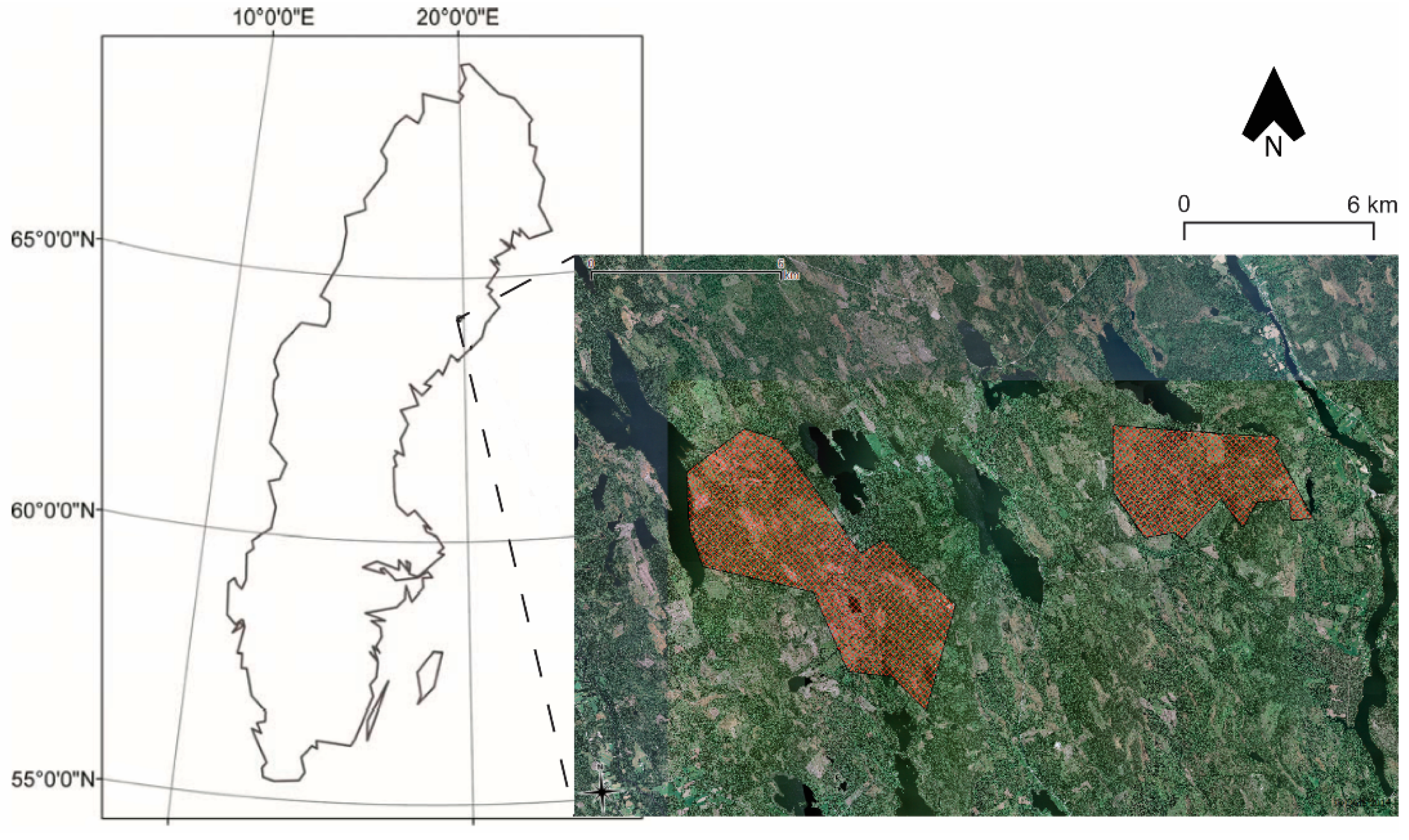
2.1. Study Area and Design

We sampled laser-scanned forest stands (33 for beetles and 47 for birds; see below) ranging in age from 8–130 years and located in a 30 km × 40 km large forest landscape in the middle boreal zone [58] of northern Sweden (64°05′–64°10′N, 19°05′–19°30′E; Figure 1).
Figure 1. The location of the study area in Sweden and an orthophoto with the laser-scanned areas drawn in red.
Remotesensing 07 04233 g001
Slightly more than two-thirds of the study stands were younger than 60 years. These originated from clear cutting and have been regenerated predominantly with two conifers: Scots pine (Pinus sylvestris) and Norway spruce (Picea abies). Among these stands, those established in the 1950s–1960s included the oldest available stands originating from past clear-cutting. Older stands included in the study have never been clear-cut, but they have been subjected to selective felling and thinning. All study sites were separated by at least 500 m, and stands of different ages were spatially interspersed. Mean stand size was 18 ha (range 4–35 ha), and birds and beetles were surveyed within a circle with a 50-m radius in each stand (see below), placed within each stand in such a way as to cover a homogenous forest area.
The dominant forest site types [59] in the stands were of mesic and moist dwarf-shrub type, both with Vaccinium myrtillus L. as the dominant species in the field layer and the more productive herb dwarf-shrub type with some meadow herbs (Geranium silvaticum, Oxalis acetosella) and grasses. The tree layer was dominated by a mixture of Scots pine and Norway spruce with a minor component of birch (Betula pubescens and B. pendula), Eurasian aspen (Populus tremula), goat willow (Salix caprea) and grey alder (Alnus incana). The management histories of the stand types were reflected in a gradually decreasing proportion of the early-successional Scots pine from younger to older stands. Deciduous trees were most abundant in young stands, reflecting the fact that the deciduous species found in the study area are all shade-intolerant pioneers. The late-successional Norway spruce showed the opposite pattern, being most abundant in older stands.

2.2. Beetle Sampling

We sampled beetles in a total of 42 stands, of which 9 lay outside of the ALS-scanned area, yielding a final set of 33 study stands with both beetle and ALS data. All analyses based on the beetle data (involving ALS and/or kNN variables; see below) were based on these 33 stands. In each study stand, we deployed 10 pitfall traps between 14 June and 5 August 2009 and three IBL2® window (i.e., flight interception) traps between 14 June and 16 September 2009. The pitfall traps consisted of a 150-mL plastic container (ø 65 mm) buried so that the edge was level with the ground. To prevent rain water from flooding the traps, we placed a metal roof five cm above each trap. In each of the stands, pitfall traps were placed with one trap at the center of the survey circle and the rest in three transects comprising three traps each, heading north, southwest and southeast from the center. The between-trap distance along the transects was 15 m.
In each site, the three IBL2® window traps, each with a flight intercept surface of 0.35 m2, were placed at a height of 1.5–2 m, 50 m from each other in a triangle centered on the stand’s midpoint to cover different flight directions. The insect traps were filled with 70% propylene glycol to preserve the insects and some detergent to reduce surface tension [60]. All beetles were sent to an expert taxonomist for determination. Nomenclature and taxonomy of beetles follow Silfverberg [61].

2.3. Bird Sampling

We surveyed birds in a total of 62 stands, of which 15 lay outside of the ALS-scanned area, yielding a final set of 47 study stands with both bird and ALS data. All analyses based on the bird data (involving ALS and/or kNN variables; see below) were based on these 47 stands, of which 33 were also used for the beetle models. We used point counts with a fixed radius of 50 m and an observation time of 7.5 min per visit. Each point count station was visited 6 times in total, in mornings with favorable weather conditions (i.e., no strong wind or rain), three times during the early spring (1 April–7 May 2010; from 05:30 to 10:30 a.m.) and three times during the late spring (25 May to 20 June 2009; from 04:00 to 09:00 a.m.). We recorded all bird individuals heard or seen within the 50-m observation radius, except birds flying over the plot without landing. Based on the data from all six visits for resident species and the three late-spring visits for migrants, we estimated the number of breeding pairs for each species at each point count station.

2.4. Forest Estimates Derived from Satellite Images

We extracted data from kNN-Sweden 2010, which provides estimates of forest age, basal area-weighted tree height, total stem volume and the proportions of different tree species in a raster with a resolution of 25 m × 25 m [62]. The forest estimates are based on forest data from the Swedish National Forest Inventory (NFI) combined with satellite images from SPOT 4 and SPOT 5 [17]. The estimation is done with k nearest neighbors (kNN) imputation from the digital numbers of the satellite images. The estimates are most accurate for stem volume and slightly less accurate for tree species and tree height in middle-aged and old forest [17].
Variables describing the forest conditions were derived as mean values across all 25 m × 25-m raster cells within circles of a 50-m radius (i.e., within a homogenous forest stand) and a 200-m radius (i.e., including also parts of adjacent stands) with the same center as the survey circles (Table 1). A given raster cell was included if its center fell inside the circle.
Table 1. Summary description of the initial set of variables derived from kNN and ALS. All variables depict the mean value (and standard deviation in the case of ALS_MaxHsd) calculated across all raster cells encompassed by the study plot. Each variable exists in two variants corresponding to the two radii where the explanatory variables were extracted from the initial raster: 50 and 200 m. Elsewhere in the article, the radius is specified by adding a suffix to the variable name (e.g., kNN_Age50).
VariableDescriptionInitial Raster Cell Size (m × m)
kNN-Based Variables
kNN_AgeMean estimated forest age25 × 25
kNN_HeightMean estimated tree height25 × 25
kNN_PineMean estimated proportion of Scots pine stem volume25 × 25
kNN_SpruceMean estimated proportion of Norway spruce stem volume25 × 25
kNN_DeciduousMean estimated proportion of deciduous (i.e., broadleaved) tree stem volume25 × 25
kNN_VolumeMean estimated total stem volume25 × 25
ALS-Based Variables
ALS_95HeightMean of the 95th percentile of height above the ground10 × 10
ALS_HighVegMean of the fraction of returns ≥ 3 m above the ground of all returns10 × 10
ALS_LowVegMean of the fraction of returns ≥ 0.5 m above the ground of all returns ≤ 3 m above the ground10 × 10
ALS_ShanHMean of Shannon’s diversity index for height10 × 10
ALS_MaxHMean of the maximum height1 × 1
ALS_MaxHsdStandard deviation of the maximum height1 × 1

2.5. ALS Data

The ALS data were acquired on 3 and 5 August 2008, using a TopEye system S/N 425 with a wavelength of 1064 nm and a flying altitude of 500 m above the ground. The first and last returns were saved for each laser pulse, and the average density of returns was 5 m−2. Laser returns were classified as ground or non-ground, and the ground returns were used to derive a digital elevation model (DEM) with 0.5-m raster cells. The height above the ground was calculated for each laser return by subtracting the height of the DEM.
The following metrics were calculated from the ALS data including all returns for each 10 m × 10 m raster cell (i.e., large enough to contain several trees per cell) within the study radius:
  • The 95th percentile of vegetation height above the ground (95Height). This variable depicts a general measure of the canopy height.
  • The fraction of returns ≥ 3 m above the ground of all returns (HighVeg). This represents a general measure of higher-level foliage density, i.e., excluding vegetation below 3 m.
  • The fraction of returns ≥ 0.5 m above the ground of all returns ≤ 3 m above the ground (LowVeg). This represents a general measure of lower-level foliage density below 3.0 m.
  • Shannon’s diversity index for the proportion of returns in height intervals 0.5–3 m, 3–10 m and 10–35 m above the ground within each raster cell (ShanH). This provides an index of foliage height diversity (sensu [63]).
In addition to the above-mentioned variables, we derived maximum vegetation height (MaxH) for 1 m × 1 m cells (i.e., to capture the variation at the tree level). We then calculated the mean value of ALS_MaxH across all 1 m × 1 m raster cells in the 50-m and 200-m circles. Here, we also calculated the standard variation across cells to provide an index of the fine-scale variation in the height of the top of the forest canopy. The ALS variables were derived as mean values across all 10 m × 10 m or 1 m × 1 m raster cells in circles with a 50-m and 200-m radius centered on the study stands (Table 1), which is similar to methods used in earlier studies (e.g., [52,64,65,66,67]).

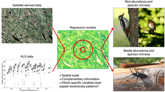
2.6. Regression Models

To test if ALS data or satellite-derived data products, or a combination of the two, can be used to identify important habitats for forest-dwelling beetles and birds in boreal forests, linear regression models with log-log transformations were fitted for the species richness and abundance of birds, beetles caught in the flight interception traps (“flying beetles”) and beetles caught in the pitfall traps (“epigaeic beetles”), respectively, as functions of the forest structure variables derived from kNN and ALS. We chose to use linear regression, because this is a parametric model that allows a biological interpretation of the results. The log-log transformations were based on the assumption of a multiplicative relationship between the response variables and the explanatory variables. The explanatory variables were transformed with the logarithm of the variable plus two, and the response variable was transformed with the logarithm of the variable plus one with the assumption that multiplicative models would fit best. To avoid issues of multicollinearity, only explanatory variables with a Pearson correlation coefficient ≤ 0.6 were retained for the analyses (Table 2) [68]. To achieve that, we removed the variables that were correlated with the highest number of other variables. The variables ALS_MaxH and kNN_Volume were strongly correlated with each other, but not with other variables. Considering the potential ecological importance of these two variables representing the ALS and kNN data, respectively, we included each of them separately in the model selection process. Hence, for each response variable and radius, we used one set of candidate explanatory variables including ALS_MaxH and another including kNN_Volume. Separate models were created for the 50-m and 200-m radius. For each response variable and radius, the best model was selected based on the Akaike information criterion corrected for finite sample sizes (AICc) [68].
To study the ability of the models to predict species richness and abundance in the whole study area, we also performed leave-one-out cross-validation [69]: one field plot was excluded from the dataset; the models were estimated based on the remaining field plots; and the resulting model was used to estimate the species richness and abundance of the excluded field plot. The root mean squared error (RMSE) and bias were calculated from the results of Equations (1) and (2).
R M S E = i = 1 n ( Y ^ i Y i ) 2 n
B i a s = i = 1 n ( Y ^ i Y i ) n
where Yi is the field-observed species richness or abundance, Y ^ i is the estimated value in plot i and n is the total number of plots. The RMSE is a measure of the error of the estimated species richness and abundance.
Table 2. Final set of candidate explanatory variables used for model selection (see Table 1 for variable descriptions). For each of the two radii, model selection was performed separately for one set of candidate variables including ALS_MaxH and for another including kNN_Volume.
50-m Radius200-m Radius
ALS_ShanH 50ALS_ShanH 200
ALS_LowVeg 50ALS_LowVeg 200
ALS_MaxH 50 or kNN_Volume 50ALS_MaxH 200 or kNN_Volume 200
kNN_Deciduous 50kNN_Height 200
kNN_Pine 50kNN_Deciduous 200
kNN_Pine 200
To summarize the amount of evidence for each of the explanatory variables and, hence, to identify the variables that best explained species richness and the abundance of birds and beetles, we calculated the sum of AICc model weights for each variable across all models [68], separately for the sets of models with ALS_MaxH and those with kNN_Volume. As the models at the 50-m radius consistently performed better than the 200-m radius (see the Results Section), we only calculated the AICc weights for the models at 50 m.

3. Results

Both the kNN and ALS variables could explain a large proportion of the variation in species richness for birds and beetles. The explanatory power (i.e., adjusted R-squared) of the lowest-AICc models was relatively high, and it was higher for abundance and species richness of beetles than birds (Table 3). The highest explanatory power was found for species richness of epigaeic beetles (adj. R2 = 0.59). For each of the six response variables, the most parsimonious model based on variables derived within the 50-m radius had lower AICc and better explanatory power than the one based on the 200-m radius. The RMSE calculated with leave-one-out cross-validation followed the same pattern: the RMSE was lower for the 50-m radius than for the 200-m radius. For the epigaeic and flying beetles, the bias was close to zero. For the birds, the bias was rather large and negative, although it was similar for the two radii.
For the 50-m radius, the models based on the set of candidate variables including ALS_MaxH50 performed better based on AICc than the ones including kNN_Volume50 in all cases. For the 200-m radius, the models including ALS_MaxH200 had a lower AICc than those including kNN_Volume200 in all cases, except one (i.e., epigaeic beetle abundance).
Table 3. Models with the lowest corrected AIC (AICc) based on all possible combinations of the explanatory variables listed in Table 2 for each of the two radii.
50 m Radius200 m Radius
Regression ModelAdjusted R2AICcRMSE (Cross-Validation)Bias (Cross-Validation)Regression ModelAdjusted R2AICcRMSE (Cross-Validation)Bias (Cross-Validation)
Bird abundance+ALS_LowVeg50 ***
+ALS_MaxH50 ***
0.4233.635.8%−16.7%+ALS_LowVeg200 *
+ALS_MaxH200 ***
0.2148.037.9%−16.7%
Bird species richness+ALS_LowVeg50 **
+ALS_MaxH50 ***
0.4129.634.8%−17.4%+ALS_LowVeg200 *
+ALS_MaxH200 **
0.2044.136.8%−17.5%
Flying beetle abundance−kNN_Pine50 *
+ALS_MaxH50 ***
0.5333.139.6%−0.2%−kNN_Pine200 *
+ ALS_MaxH200 **
0.3842.645.7%0.0%
Flying beetle species richness−kNN_Pine50 *
+ALS_MaxH50 ***
0.476.223.5%−0.6%−kNN_Pine200 ns
+ALS_MaxH200 **
0.2816.226.9%−0.7%
Epigaeic beetle abundance+ALS_MaxH50 ***0.5373.977.5%−0.5%+kNN_Volume200 ***0.4578.983.0%−0.5%
Epigaeic beetle species richness−kNN_Pine50 *
+ALS_MaxH50 ***
0.5929.532.9%−1.2%−kNN_Pine200 **
+ ALS_MaxH200 ***
0.5730.336.5%−0.8%
*** p < 0.001; ** p < 0.01; * p < 0.05; ns p > 0.1.
For all six response variables, the variables ALS_MaxH50 and kNN_Volume50 had the highest sum of AICc model weights among all predictors in their respective sets of models (50-m radius; Table 4 and Table 5). The sign of these two variables was positive. For bird abundance and species richness, the variable ALS_LowVeg50 had the second highest sum of AICc model weights with a positive sign. For flying and epigaeic beetle abundance and richness, the variable kNN_Pine50 had the second highest sum of AICc model weights with a negative sign for four response variables where ALS_MaxH50 was included as a candidate variable (Table 4).
Table 4. Explanatory variables with the sum of AICc model weights and their signs for models at the 50-m radius including ALS_MaxH50.
kNN_Deciduous50kNN_Pine50ALS_MaxH50ALS_LowVeg50ALS_ShanH50
Bird abundance0.26 (−)0.27 (−)1.00 (+)0.99 (+)0.22 (−)
Bird species richness0.27 (−)0.23 (−)1.00 (+)0.98 (+)0.22 (−)
Flying beetle abundance0.23 (+)0.89 (−)0.99 (+)0.43 (−)0.23 (+)
Flying beetle species richness0.21 (+)0.72 (−)0.99 (+)0.24 (−)0.22 (−)
Epigaeic beetle abundance0.26 (+)0.34 (−)1.00 (+)0.25 (+)0.23 (−)
Epigaeic beetle species richness0.22 (+)0.91 (−)0.99 (+)0.22 (+)0.70 (−)
Table 5. Explanatory variables with the sum of AICc model weights and their signs for models at the 50-m radius including kNN_Volume50.
kNN_Deciduous50kNN_Pine50kNN_Volume50ALS_LowVeg50ALS_ShanH50
Bird abundance0.30 (−)0.23 (−)1.00 (+)0.73 (+)0.23 (+)
Bird species richness0.31 (−)0.22 (+)1.00 (+)0.68 (+)0.23 (−)
Flying beetle abundance0.21 (+)0.71 (−)0.92 (+)0.84 (−)0.27 (+)
Flying beetle species richness0.23 (−)0.55 (−)0.84 (+)0.54 (−)0.32 (−)
Epigaeic beetle abundance0.20 (+)0.22 (−)1.00 (+)0.25 (−)0.21 (−)
Epigaeic beetle species richness0.20 (+)0.46 (−)0.98 (+)0.24 (−)0.31 (−)

4. Discussion

4.1. Can ALS and Satellite-Derived Data Products Be Used to Identify Species Richness and Abundance Hotspots for Beetles and Birds in Managed Boreal Forest?

The facts that the best regression models based on ALS and satellite-derived data products were statistically significant and had relatively high explanatory power suggest that relatively simple models containing one or two ALS or satellite-derived variables have potential for being used to identify patches with high species richness or abundance of birds and beetles in boreal forest landscapes. Our findings are in accordance with the results of studies performed in temperate forests [50,51,66,67,70], as well as with a recent study linking ALS data and bird species richness at boreal latitudes [52]. Hence, the fine-grained quantification of habitat structure allowed by ALS data can be useful for predicting species richness patterns in birds [50].
The satellite-derived data products were forest estimates based on forest data from the Swedish NFI combined with satellite images. Alternatively, the models could also have been defined as functions of information derived directly from the satellite images, for example NDVI. This would require either a thorough analysis of the mathematical relation between the response and explanatory variables or the use of non-parametric models. One advantage of using the forest estimates as explanatory variables is that a biological interpretation of the models is possible, in particular with parametric models, such as linear regression.

4.2. Do the Models Perform Better When the Explanatory Variables Are Derived at the Scale of Homogenous Forest Stands or at a Scale Including Also Parts of Adjacent Stands?

The superior performance of models based on vegetation data from a 50-m radius compared to a 200-m radius suggests that birds and beetles are most strongly influenced by forest structure in the immediate vicinity of the sampling site. Ranius et al. [71] found that the spatial scale at which beetle and bug (Hemiptera) species on average had their strongest response to habitat characteristics was 93 m. However, a recent review of how habitat characteristics at different scales influence species richness in saproxylic species reports large variation in patterns between taxonomic groups [72]. Our results indicate that a radius of 200 m encompasses a too large of an area to detect a strong relation between forest structure and bird/beetle species richness. This is probably a consequence of the rather fine spatial grain of our study landscape: the area encompassed by a radius of 50 m was always confined to a forest patch with rather homogenous characteristics, whereas a radius of 200 m typically included forest whose age, height and vegetation structure may have differed widely from the area where the bird/beetle data were collected. Other bird studies indicate that local stand variables are important predictors of bird species richness, although some also highlight the importance of the broader landscape context [50,73]. As such, our results do not contradict previous findings, highlighting the importance of the landscape context for explaining local biodiversity patterns (e.g., [14,74]), because we did not specifically evaluate additional effects of the landscape context after accounting for local-scale conditions. Additionally, although 50 m performed better, it is not necessarily the optimal radius, and more research would be needed to determine the best radius. Still, our results highlight the importance of matching the scale of the data with that of the ecological response.

4.3. Do ALS and Satellite-Derived Data Products Provide Complementary Types of Information for Predicting Biodiversity Patterns?

The fact that all best models for a 50-m radius (and all but one at the 200-m radius) contained ALS variables suggests that ALS data can improve our ability to predict species richness and abundance of birds and beetles substantially compared to commonly-used satellite-derived data products. For birds, the best models contained ALS-derived variables only. Studies from North America also indicate that ALS is very useful for explaining pattern of species richness in birds [50]. For beetles, our results indicate that a combination of ALS data about forest height and satellite-derived data products depicting tree species composition would provide the best explanatory power. This is consistent with past findings that tree species composition is an important predictor of species richness in beetles [75]. Hence, ALS and the satellite-derived data products may provide largely complementary information of value for describing forest habitats, with ALS providing fine-resolution data about vertical forest structure and the satellite-derived data products providing information about tree species composition, which is harder to derive from ALS (e.g., [76,77]).

4.4. Which Specific Variables Derived from These Two Remote Sensing Sources Can Best Explain Biodiversity Patterns for Beetle and Bird Species in Managed Boreal Forests?

The approach to calculate the sum of AICc model weights for each variable across all models meant that all possible combinations of explanatory variables were included: ALS only, satellite-derived only and combinations of ALS and satellite-derived variables. For a radius of 50 m, the best model for all six response variables contained the variable ALS_MaxH, and this variable had the highest sum of AICc weights across models. Similarly, kNN_Volume had the highest sum of AICc weights for all models where it was used instead of ALS_MaxH. ALS_MaxH describes the mean height of the forest, whereas kNN_Volume describes the mean stem volume, both of which generally increase with the age of the forest. The higher sum of AICc weights for the models where ALS_MaxH was used can be related to the higher accuracy of that variable compared to kNN_Volume. One possible explanation for the positive relationship between the forest height or volume and species richness is that tall or high-volume forest is expected to hold larger amounts of green biomass and, hence, provide more productive energy for birds and insects, which, in turn, may result in larger numbers of individuals and higher species richness [78]. Moreover, older forest usually contains higher abundances of rare substrates, such as dead wood and dying trees [34], which are important for many boreal beetle and bird species [79,80,81]. In a study from Canada, Janssen et al. [82] found that the species richness of flying beetles increased with the basal area of large trees, the amount of dead wood and the heterogeneity of the tree species composition. Overall, our findings are in accordance with previous studies showing a positive correlation between forest age and the species richness of beetles [23,24], birds [83] and other taxonomic groups [15].
The importance and positive sign of the variable ALS_LowVeg for abundance and species richness of birds suggests that a high density of low vegetation benefits bird diversity. This is consistent with previous studies showing that many boreal forest bird species perform better in layered stands [33]. Previous studies including ALS data have also found a positive correlation between bird species richness and the density of low vegetation [51], as well as canopy and midstory height and midstory density [84], although different bird guilds seem to benefit from different forest structures [19,51,84,85].
The negative sign of the variable kNN_Pine for flying and epigaeic beetle abundance and richness suggests that a smaller proportion of pine benefits those species. This is consistent with existing knowledge about the habitat needs of these species. For example, the number of wood-living species associated with Scots pine is lower than for Norway spruce in Fennoscandia [86]. Furthermore, pine is usually associated with sites of lower productivity than spruce, which might also contribute to lower numbers of species and individuals in pine-dominated sites [87]. The negative relationship could also be related to the lower proportion of pine in older forest stands in the study area. However, the dependence on the age and size of the trees was accounted for, since the models also included ALS_MaxH or kNN_Volume.
The regression models included only a subset of the original variables derived from the remotely-sensed data since some variables were removed to avoid multicollinearity issues. All removed variables had a strong positive correlation with ALS_MaxH and kNN_Volume. The removed variables were related to forest height and forest age, but also to the proportion of Norway spruce and the density of vegetation ≥ 3 m above the ground. Since ALS_MaxH and kNN_Volume were the most important explanatory variables based on AICc, the biodiversity patterns may alternatively be explained by forest age, the proportion of Norway spruce and the density of vegetation ≥ 3 m above the ground.
A recent review of ecosystem mapping from ALS data found that increased structural heterogeneity in the canopy layer favored most flying vertebrate species, while canopy height and cover and the density of understory vegetation showed mixed results for bird and bat diversity, although several studies reported that bird diversity and individual bird species increased with increasing understory plant density [19], which is consistent with our results. The same review found that the most important property for beetle biodiversity was variability in the canopy height. In our study, the explanatory variable expressing this, ALS_MaxHsd, was removed due to its high correlation with ALS_MaxH, which was the most important variable in the models. Our study included both ALS data and forest estimates derived from satellite images, which enabled comparison of the data sources, as well as a biological interpretation of the satellite-derived variables.

5. Conclusions

Information derived from remotely-sensed data (ALS data and satellite-derived data products) can clearly be used to identify habitats associated with high species richness and abundance of forest-dwelling beetles and birds in boreal forest.
Satellite-derived data products and ALS data provide useful information for explaining stand-scale biodiversity patterns in beetles (R2 = 0.47–0.59) and to a somewhat lesser extent in birds (R2 = 0.41–0.42). Mean canopy height and total stem volume, which are largely indicative of forest age, were positively related to bird and insect species richness. A likely explanation is that older forests usually hold larger amounts of critical resources for bird and beetle species, especially if they have never been clear-felled. The models based on variables derived within the 50-m radius had lower AICc (average 26%–29%) and better explanatory power (average 57%–91%) than those based on the 200-m radius.
For the 50-m radius, the mean canopy height derived from ALS data performed better based on AICc than the mean total stem volume from kNN (average 17%).
For birds, the second highest sum of AICc model weights was found for the density of low vegetation derived from ALS data (0.98–0.99 and 0.68–0.73) with a positive sign. This suggests that denser low vegetation benefits bird species richness and abundance. For flying beetles and epigaeic beetles, the second highest sum of AICc model weights was found for the estimated proportion of pine from kNN (0.72–0.91 and 0.46–0.71) with a negative sign in three models. This suggests that a smaller proportion of pine benefits those species. In our models, ALS data contributed mostly with information about the structure and height of the forest vegetation, while the satellite-derived data products contributed with information about the tree species composition of importance for beetles.
Based on our findings, we encourage researchers and managers to utilize remotely-sensed data to identify potential biodiversity hotspots across boreal landscapes. Combining ALS data with satellite images could provide an effective tool for identifying areas that should be prioritized as set-asides or core areas in forest conservation planning.

Acknowledgments

This study was funded by The Swedish Research Council for Environment, Agricultural Sciences and Spatial Planning (FORMAS, Eva Lindberg), Future Forests (Joakim Hjältén and Jean-Michel Roberge), the Swedish Energy Agency (Therese Johansson) and the Swedish Governmental Agency for Innovation Systems (VINNOVA, Therese Johansson). Stig Lundberg and Jacek Hilszczanski determined the beetles. Aron Sandling, Antoine Bos, Oskar Söderback, Alexander Hjältén, Adrian Hjältén, Caroline Letzner, Fredrik Stenbacka and Nina Stenbacka helped out in the field. We thank Sveaskog for providing field sites and Tomas Hörnlund for maps and stand database information. We also thank Stiftelsen Gunnar och Birgitta Nordins fond for supporting the project (The Royal Swedish Academy of Agriculture and Forestry, Grant Number H14-0081-GBN).

Author Contributions

JMR, TJ and JH collected the field data. EL, JMR, TJ and JH designed the research, analyzed the data and wrote the paper. All authors read and approved the final manuscript.

Conflicts of Interest

The authors declare no conflict of interest.

References

  1. Harrison, S.; Bruna, E. Habitat fragmentation and large-scale conservation: What do we know for sure? Ecography 1999, 22, 225–232. [Google Scholar] [CrossRef]
  2. Pimm, S.L.; Jenkins, C.N.; Abell, R.; Brooks, T.M.; Gittleman, J.L.; Joppa, L.N.; Raven, P.H.; Roberts, C.M.; Sexton, J.O. The biodiversity of species and their rates of extinction, distribution, and protection. Science 2014, 344. [Google Scholar] [CrossRef]
  3. Esseen, P.-A.; Ehnström, B.; Ericson, L.; Sjöberg, K. Boreal forests. In Ecological Bulletins, Boreal Ecosystems and Landscapes: Structures, Processes and Conservation of Biodiversity; Hansson, L., Ed.; Oikos Editorial Office: Lund, Sweden, 1997; Volume 46, pp. 16–47. [Google Scholar]
  4. Linder, P.; Östlund, L. Structural changes in three mid-boreal Swedish forest landscapes, 1885–1996. Biol. Conserv. 1998, 85, 9–19. [Google Scholar] [CrossRef]
  5. Siitonen, J. Forest management, coarse woody debris and saproxylic organisms: Fennoscandian boreal forest as an example. Ecol. Bull. 2001, 49, 11–41. [Google Scholar]
  6. Gibb, H.; Ball, J.P.; Johansson, T.; Atlegrim, O.; Hjältén, J.; Danell, K. Effects of management on coarse woody debris volume and composition in boreal forests in northern Sweden. Scand. J. For. Res. 2005, 20, 213–222. [Google Scholar] [CrossRef]
  7. Grove, S.J. Saproxylic insect ecology and the sustainable management of forests. In Annual Review of Ecology and Systematics; Futuyma, D.J., Ed.; Annual Reviews: Palo Alto, CA, USA, 2002; Volume 33, pp. 1–23. [Google Scholar]
  8. Harmon, M.E.; Franklin, J.F.; Swanson, F.J.; Sollins, P.; Gregory, S.V.; Lattin, J.D.; Anderson, N.H.; Cline, S.P.; Aumen, N.G.; Sedell, J.R.; et al. Ecology of coarse woody debris in temperate ecosystems. Adv. Ecol. Res. 1986, 15, 133–302. [Google Scholar]
  9. Niklasson, M.; Granström, A. Numbers and sizes of fires: Long-term spatially explicit fire history in a Swedish boreal landscape. Ecology 2000, 81, 1484–1499. [Google Scholar] [CrossRef]
  10. Larsson, S.; Danell, K. Science and the management of boreal forest biodiversity—Preface. Scand. J. For. Res. 2001, 16, 5–9. [Google Scholar] [CrossRef]
  11. Angelstam, P.; Roberge, J.M.; Ek, T.; Laestadius, L. Data and tools for conservation, management, and restoration of northern forest ecosystems at multiple scales. In Restoration of Boreal and Temperate Forests; Stanturf, J., Madsen, P., Eds.; CRC Press: Boca Raton, FL, USA, 2005; Volume 3, pp. 269–283. [Google Scholar]
  12. Lindenmayer, D.B.; Franklin, J.F.; Fischer, J. General management principles and a checklist of strategies to guide forest biodiversity conservation. Biol. Conserv. 2006, 131, 433–445. [Google Scholar] [CrossRef]
  13. Johansson, T.; Hjältén, J.; de Jong, J.; von Stedingk, H. Environmental considerations from legislation and certification in managed forest stands: A review of their importance for biodiversity. For. Ecol. Manag. 2013, 303, 98–112. [Google Scholar] [CrossRef]
  14. Gibb, H.; Hjältén, J.; Ball, J.P.; Atlegrim, O.; Pettersson, R.B.; Hilszczanski, J.; Johansson, T.; Danell, K. Effects of landscape composition and substrate availability on saproxylic beetles in boreal forests: A study using experimental logs for monitoring assemblages. Ecography 2006, 29, 191–204. [Google Scholar] [CrossRef]
  15. Paillet, Y.; Berges, L.; Hjältén, J.; Odor, P.; Avon, C.; Bernhardt-Roemermann, M.; Bijlsma, R.-J.; de Bruyn, L.; Fuhr, M.; Grandin, U.; et al. Biodiversity differences between managed and unmanaged forests: Meta-analysis of species richness in Europe. Conserv. Biol. 2010, 24, 101–112. [Google Scholar] [CrossRef] [PubMed]
  16. Stighäll, K.; Roberge, J.-M.; Andersson, K.; Angelstam, P. Usefulness of biophysical proxy data for modelling habitat of an endangered forest species: The white-backed woodpecker dendrocopos leucotos. Scand. J. For. Res. 2011, 26, 576–585. [Google Scholar] [CrossRef]
  17. Reese, H.; Nilsson, M.; Pahen, T.G.; Hagner, O.; Joyce, S.; Tingelof, U.; Egberth, M.; Olsson, H. Countrywide estimates of forest variables using satellite data and field data from the national forest inventory. Ambio 2003, 32, 542–548. [Google Scholar] [PubMed]
  18. Martinuzzi, S.; Vierling, L.A.; Gould, W.A.; Vierling, K.T. Improving the characterization and mapping of wildlife habitats with lidar data: Measurement priorities for the inland northwest, USA. Gap Anal. Bull. 2009, 16, 1–8. [Google Scholar]
  19. Davies, A.B.; Asner, G.P. Advances in animal ecology from 3D-LiDAR ecosystem mapping. Trends Ecol. Evolut. 2014, 29, 681–691. [Google Scholar] [CrossRef]
  20. Shan, J.; Toth, C. Topographic Laser Ranging and Scanning: Principles and Processing; CRC Press/Taylor & Francis Group: Boca Raton, FL, USA, 2009. [Google Scholar]
  21. Wulder, M.A.; White, J.C.; Nelson, R.F.; Næsset, E.; Orka, H.O.; Coops, N.C.; Hilker, T.; Bater, C.W.; Gobakken, T. LiDAR sampling for large-area forest characterization: A review. Remote Sens. Environ. 2012, 121, 196–209. [Google Scholar] [CrossRef]
  22. Ussyshkin, V.; Theriault, L. Airborne LiDAR: Advances in discrete return technology for 3D vegetation mapping. Remote Sens. 2011, 3, 416–434. [Google Scholar] [CrossRef]
  23. Kraus, K.; Pfeifer, N. Determination of terrain models in wooded areas with airborne laser scanner data. ISPRS J. Photogram. Remote Sens. 1998, 53, 193–203. [Google Scholar] [CrossRef]
  24. Martinuzzi, S.; Vierling, L.A.; Gould, W.A.; Falkowski, M.J.; Evans, J.S.; Hudak, A.T.; Vierling, K.T. Mapping snags and understory shrubs for a LiDAR-based assessment of wildlife habitat suitability. Remote Sens. Environ. 2009, 113, 2533–2546. [Google Scholar] [CrossRef]
  25. Hyyppä, J.; Hyyppä, H.; Leckie, D.; Gougeon, F.; Yu, X.; Maltamo, M. Review of methods of small-footprint airborne laser scanning for extracting forest inventory data in boreal forests. Int. J. Remote Sens. 2008, 29, 1339–1366. [Google Scholar] [CrossRef]
  26. Hudak, A.T.; Evans, J.S.; Smith, A.M.S. LiDAR utility for natural resource managers. Remote Sens. 2009, 1, 934–951. [Google Scholar] [CrossRef]
  27. Stilla, U.; Jutzi, B. Waveform Analysis for Small-Footprint Pulsed Laser Systems. In Topographic Laser Ranging and Scanning: Principles and Processing; Shan, J., Toth, C., Eds.; CRC Press/Taylor & Francis Group: Boca Raton, FL, USA, 2009. [Google Scholar]
  28. Reitberger, J.; Schnorr, C.; Krzystek, P.; Stilla, U. 3D segmentation of single trees exploiting full waveform lidar data. ISPRS J. Photogram. Remote Sens. 2009, 64, 561–574. [Google Scholar] [CrossRef]
  29. Lindberg, E.; Eysn, L.; Hollaus, M.; Holmgren, J.; Pfeifer, N. Delineation of tree crowns and tree species classification from full-waveform airborne laser scanning data using 3-D ellipsoidal clustering. IEEE J. Sel. Top. Appl. Earth Observ. Remote Sens. 2014, 7, 3174–3181. [Google Scholar] [CrossRef]
  30. Polewski, P.; Yao, W.; Heurich, M.; Krzystek, P.; Stilla, U. Detection of Fallen Trees in als Point Clouds by Learning the Normalized Cut Similarity Function from Simulated Samples. ISPRS Ann. Photogramm. Remote Sens. Spatial Inf. Sci. 2014, II-3, 111–118. [Google Scholar] [CrossRef]
  31. Whitehurst, A.S.; Swatantran, A.; Blair, J.B.; Hofton, M.A.; Dubayah, R. Characterization of canopy layering in forested ecosystems using full waveform LiDAR. Remote Sens. 2013, 5, 2014–2036. [Google Scholar] [CrossRef]
  32. Camprodon, J.; Brotons, L. Effects of undergrowth clearing on the bird communities of the northwestern mediterranean coppice holm oak forests. For. Ecol. Manag. 2006, 221, 72–82. [Google Scholar] [CrossRef]
  33. Eggers, S.; Low, M. Differential demographic responses of sympatric parids to vegetation management in boreal forest. For. Ecol. Manag. 2014, 319, 169–175. [Google Scholar] [CrossRef]
  34. Stenbacka, F.; Hjältén, J.; Hilszczanski, J.; Dynesius, M. Saproxylic and non-saproxylic beetle assemblages in boreal spruce forests of different age and forestry intensity. Ecol. Appl. 2010, 20, 2310–2321. [Google Scholar] [CrossRef] [PubMed]
  35. Niemelä, J.; Haila, Y.; Punttila, P. The importance of small-scale heterogeneity in boreal forests: Variation in diversity in forest-floor invertebrates across the succession gradient. Ecography 1996, 19, 352–368. [Google Scholar] [CrossRef]
  36. Seavy, N.E.; Viers, J.H.; Wood, J.K. Riparian bird response to vegetation structure: A multiscale analysis using LiDAR measurements of canopy height. Ecol. Appl. 2009, 19, 1848–1857. [Google Scholar] [CrossRef] [PubMed]
  37. Zellweger, F.; Braunisch, V.; Baltensweiler, A.; Bollmann, K. Remotely sensed forest structural complexity predicts multi species occurrence at the landscape scale. For. Ecol. Manag. 2013, 307, 303–312. [Google Scholar] [CrossRef]
  38. Coops, N.C.; Waring, R.H.; Wulder, M.A.; Pidgeon, A.M.; Radeloff, V.C. Bird diversity: A predictable function of satellite-derived estimates of seasonal variation in canopy light absorbance across the United States. J. Biogeogr. 2009, 36, 905–918. [Google Scholar] [CrossRef]
  39. Coops, N.C.; Wulder, M.A.; Iwanicka, D. Exploring the relative importance of satellite-derived descriptors of production, topography and land cover for predicting breeding bird species richness over Ontario, Canada. Remote Sens. Environ. 2009, 113, 668–679. [Google Scholar] [CrossRef]
  40. Goetz, S.J.; Sun, M.; Zolkos, S.; Hansen, A.; Dubayah, R. The relative importance of climate and vegetation properties on patterns of north American breeding bird species richness. Environ. Res. Lett. 2014, 9. [Google Scholar] [CrossRef]
  41. Sheeren, D.; Bonthoux, S.; Balent, G. Modeling bird communities using unclassified remote sensing imagery: Effects of the spatial resolution and data period. Ecol. Indic. 2014, 43, 69–82. [Google Scholar] [CrossRef]
  42. Shirley, S.M.; Yang, Z.; Hutchinson, R.A.; Alexander, J.D.; McGarigal, K.; Betts, M.G. Species distribution modelling for the people: Unclassified landsat tm imagery predicts bird occurrence at fine resolutions. Divers. Distrib. 2013, 19, 855–866. [Google Scholar] [CrossRef]
  43. Culbert, P.D.; Radeloff, V.C.; St-Louis, V.; Flather, C.H.; Rittenhouse, C.D.; Albright, T.P.; Pidgeon, A.M. Modeling broad-scale patterns of avian species richness across the midwestern United States with measures of satellite image texture. Remote Sens. Environ. 2012, 118, 140–150. [Google Scholar] [CrossRef]
  44. St-Louis, V.; Pidgeon, A.M.; Kuemmerle, T.; Sonnenschein, R.; Radeloff, V.C.; Clayton, M.K.; Locke, B.A.; Bash, D.; Hostert, P. Modelling avian biodiversity using raw, unclassified satellite imagery. Philos. Trans. R. Soc. B-Biol. Sci. 2014, 369. [Google Scholar] [CrossRef]
  45. Wood, E.M.; Pidgeon, A.M.; Radeloff, V.C.; Keuler, N.S. Image texture predicts avian density and species richness. PLoS ONE 2013, 8. [Google Scholar] [CrossRef] [PubMed]
  46. Goetz, S.; Steinberg, D.; Dubayah, R.; Blair, B. Laser remote sensing of canopy habitat heterogeneity as a predictor of bird species richness in an eastern temperate forest, USA. Remote Sens. Environ. 2007, 108, 254–263. [Google Scholar] [CrossRef]
  47. Simonson, W.D.; Allen, H.D.; Coomes, D.A. Applications of airborne lidar for the assessment of animal species diversity. Methods Ecol. Evol. 2014, 5, 719–729. [Google Scholar] [CrossRef]
  48. Hill, R.A.; Hinsley, S.A.; Broughton, R.K. Assessing habitats and organism-habitat relationships by airborne laser scanning. In Forestry Applications of Airborne Laser Scanning: Concepts and Case Studies; Maltamo, M., Naesset, E., Vauhkonen, J., Eds.; Springer: Dordrecht, The Netherlands, 2014; Volume 27, pp. 335–356. [Google Scholar]
  49. Müller, J.; Vierling, K. Assessing biodiversity by airborne laser scanning. In Forestry Applications of Airborne Laser Scanning: Concepts and Case Studies; Maltamo, M., Naesset, E., Vauhkonen, J., Eds.; Springer: Dordrecht, The Netherlands, 2014; Volume 27, pp. 357–374. [Google Scholar]
  50. Weisberg, P.J.; Dilts, T.E.; Becker, M.E.; Young, J.S.; Wong-Kone, D.C.; Newton, W.E.; Ammon, E.M. Guild-specific responses of avian species richness to lidar-derived habitat heterogeneity. Acta Oecol. 2014, 59, 72–83. [Google Scholar] [CrossRef]
  51. Vogeler, J.C.; Hudak, A.T.; Vierling, L.A.; Evans, J.; Green, P.; Vierling, K.I.T. Terrain and vegetation structural influences on local avian species richness in two mixed-conifer forests. Remote Sens. Environ. 2014, 147, 13–22. [Google Scholar] [CrossRef]
  52. Eldegard, K.; Dirksen, J.W.; Ørka, H.O.; Halvorsen, R.; Næsset, E.; Gobakken, T.; Ohlson, M. Modelling bird richness and bird species presence in a boreal forest reserve using airborne laser-scanning and aerial images. Bird Study 2014, 61, 204–219. [Google Scholar] [CrossRef]
  53. Müller, J.; Moning, C.; Bässler, C.; Heurich, M.; Brandl, R. Using airborne laser scanning to model potential abundance and assemblages of forest passerines. Basic Appl. Ecol. 2009, 10, 671–681. [Google Scholar] [CrossRef]
  54. Culbert, P.D.; Radeloff, V.C.; Flather, C.H.; Kellndorfer, J.M.; Rittenhouse, C.D.; Pidgeon, A.M. The influence of vertical and horizontal habitat structure on nationwide patterns of avian biodiversity. Auk 2013, 130, 656–665. [Google Scholar] [CrossRef]
  55. Muukkonen, P.; Angervuori, A.; Virtanen, T.; Kuparinen, A.; Merila, J. Loss and fragmentation of siberian jay (perisoreus infaustus) habitats. Boreal Environ. Res. 2012, 17, 59–71. [Google Scholar]
  56. Sirkia, S.; Helle, P.; Linden, H.; Nikula, A.; Norrdahl, K.; Suorsa, P.; Valkeajarvi, P. Persistence of capercaillie (tetrao urogallus) lekking areas depends on forest cover and fine-grain fragmentation of boreal forest landscapes. Ornis Fenn. 2011, 88, 14–29. [Google Scholar]
  57. Huang, Q.; Swatantran, A.; Dubayah, R.; Goetz, S.J. The influence of vegetation height heterogeneity on forest and woodland bird species richness across the United States. PLoS ONE 2014, 9. [Google Scholar] [CrossRef] [PubMed]
  58. Ahti, T.; Hämet-Ahti, L.; Jalas, J. Vegetation zones and their sections in northwestern Europe. Ann. Bot. Fenn. 1968, 5, 169–211. [Google Scholar]
  59. Arnborg, T. Forest types of northern Sweden. Vegetatio 1990, 90, 1–13. [Google Scholar] [CrossRef]
  60. Johansson, T.; Andersson, J.; Hjältén, J.; Dynesius, M.; Ecke, F. Short-term responses of beetle assemblages to wildfire in a region with more than 100 years of fire suppression. Insect Conserv. Divers. 2011, 4, 142–151. [Google Scholar] [CrossRef]
  61. Silfverberg, H. Enumeratio nova Coleopterorum Fennoscandiae, Daniae et Baltiae. Sahlbergia 2004, 9, 1–111, in English. [Google Scholar]
  62. Egberth, M.; Nilsson, M.; Axensten, P. kNN-Sweden—Current map data on forest land. Available online: http://skogskarta.slu.se/index.cfm?eng=1 (accessed on 21 January 2014).
  63. MacArthur, R.; MacArthur, J.W. On bird species diversity. Ecology 1961, 42, 594–598. [Google Scholar] [CrossRef]
  64. Bellamy, P.E.; Hill, R.A.; Rothery, P.; Hinsley, S.A.; Fuller, R.J.; Broughton, R.K. Willow warbler phylloscopus trochilus habitat in woods with different structure and management in southern England. Bird Study 2009, 56, 338–348. [Google Scholar] [CrossRef]
  65. Hinsley, S.A.; Hill, R.A.; Bellamy, P.E.; Harrison, N.M.; Speakman, J.R.; Wilson, A.K.; Ferns, P.N. Effects of structural and functional habitat gaps on breeding woodland birds: Working harder for less. Landsc. Ecol. 2008, 23, 615–626. [Google Scholar] [CrossRef] [Green Version]
  66. Müller, J.; Brandl, R. Assessing biodiversity by remote sensing in mountainous terrain: The potential of lidar to predict forest beetle assemblages. J. Appl. Ecol. 2009, 46, 897–905. [Google Scholar] [CrossRef]
  67. Müller, J.; Stadler, J.; Brandl, R. Composition versus physiognomy of vegetation as predictors of bird assemblages: The role of lidar. Remote Sens. Environ. 2010, 114, 490–495. [Google Scholar] [CrossRef]
  68. Burnham, K.P.; Anderson, D.R. Model Selection and Multimodel Inference: A Practical Information-Theoretic Approach; Springer: New York, NY, USA, 2002; p. 488. [Google Scholar]
  69. Geisser, S. Predictive Inference: An Introduction; Chapman & Hall: New York, NY, USA, 1993. [Google Scholar]
  70. Clawges, R.; Vierling, K.; Vierling, L.; Rowell, E. The use of airborne lidar to assess avian species diversity, density, and occurrence in a pine/aspen forest. Remote Sens. Environ. 2008, 112, 2064–2073. [Google Scholar] [CrossRef]
  71. Ranius, T.; Martikainen, P.; Kouki, J. Colonisation of ephemeral forest habitats by specialised species: Beetles and bugs associated with recently dead aspen wood. Biodivers. Conserv. 2011, 20, 2903–2915. [Google Scholar] [CrossRef]
  72. Sverdrup-Thygeson, A.; Gustafsson, L.; Kouki, J. Spatial and temporal scales relevant for conservation of dead-wood associated species: Current status and perspectives. Biodivers. Conserv. 2014, 23, 513–535. [Google Scholar] [CrossRef]
  73. Wells, K.; Boehm, S.M.; Boch, S.; Fischer, M.; Kalko, E.K.V. Local and landscape-scale forest attributes differ in their impact on bird assemblages across years in forest production landscapes. Basic Appl. Ecol. 2011, 12, 97–106. [Google Scholar] [CrossRef]
  74. Andersson, J.; Hjältén, J.; Dynesius, M. Long-term effects of stump harvesting and landscape composition on beetle assemblages in the hemiboreal forest of Sweden. For. Ecol. Manag. 2012, 271, 75–80. [Google Scholar] [CrossRef]
  75. Azeria, E.T.; Fortin, D.; Hebert, C.; Peres-Neto, P.; Pothier, D.; Ruel, J.-C. Using null model analysis of species co-occurrences to deconstruct biodiversity patterns and select indicator species. Divers. Distrib. 2009, 15, 958–971. [Google Scholar] [CrossRef]
  76. Törmä, M. Estimation of tree Species Proportions of Forest Stands Using Laser Scanning. ISPRS Int. Arch. Photogramm. Remote Sens. Spatial Inf. Sci. 2000, XXXIII((Part B7)), 1524–1531. [Google Scholar]
  77. Packalén, P.; Maltamo, M. The k-msn method for the prediction of species-specific stand attributes using airborne laser scanning and aerial photographs. Remote Sens. Environ. 2007, 109, 328–341. [Google Scholar] [CrossRef]
  78. Elo, M.; Roberge, J.-M.; Rajasarkka, A.; Monkkonen, M. Energy density and its variation in space limit species richness of boreal forest birds. J. Biogeogr. 2012, 39, 1462–1472. [Google Scholar] [CrossRef]
  79. Gibb, H.; Johansson, T.; Stenbacka, F.; Hjältén, J. Functional roles affect diversity-succession relationships for boreal beetles. PLoS ONE 2013, 8. [Google Scholar] [CrossRef] [PubMed]
  80. Hjältén, J.; Stenbacka, F.; Pettersson, R.B.; Gibb, H.; Johansson, T.; Danell, K.; Ball, J.P.; Hilszczanski, J. Micro and macro-habitat associations in saproxylic beetles: Implications for biodiversity management. PLoS ONE 2012, 7. [Google Scholar] [CrossRef] [PubMed]
  81. Roberge, J.-M.; Angelstam, P.; Villard, M.-A. Specialised woodpeckers and naturalness in hemiboreal forests—Deriving quantitative targets for conservation planning. Biol. Conserv. 2008, 141, 997–1012. [Google Scholar] [CrossRef]
  82. Janssen, P.; Fortin, D.; Hebert, C. Beetle diversity in a matrix of old-growth boreal forest: Influence of habitat heterogeneity at multiple scales. Ecography 2009, 32, 423–432. [Google Scholar] [CrossRef]
  83. Helle, P. Effects of forest regeneration on the structure of bird communities in northern Finland. Holarct. Ecol. 1985, 8, 120–132. [Google Scholar]
  84. Lesak, A.A.; Radeloff, V.C.; Hawbaker, T.J.; Pidgeon, A.M.; Gobakken, T.; Contrucci, K. Modeling forest songbird species richness using LiDAR-derived measures of forest structure. Remote Sens. Environ. 2011, 115, 2823–2835. [Google Scholar] [CrossRef]
  85. Jones, T.G.; Arcese, P.; Sharma, T.; Coops, N.C. Describing avifaunal richness with functional and structural bioindicators derived from advanced airborne remotely sensed data. Int. J. Remote Sens. 2013, 34, 2689–2713. [Google Scholar] [CrossRef]
  86. Dahlberg, A.; Stokland, J.N. Vedlevande Arters Krav på Substrat—en Sammanställning Och Analys av 3600 Arter (in Swedish with English summary: Substrate Requirements of Wood-Inhabiting Species—A Synthesis and Analysis of 3600 Species); Skogsstyrelsen: Jönköping, Sweden, 2004. [Google Scholar]
  87. Bernes, C. Biologisk Mångfald i Sverige. Monitor 22 (Biodiversity in Sweden. Monitor 22); Naturvårdsverket/The Swedish Environment Protection Agency: Stockholm, Sweden, 2011. [Google Scholar]

