Using Optical Satellite Data and Airborne Lidar Data for a Nationwide Sampling Survey

Abstract

A workflow for combining airborne lidar, optical satellite data and National Forest Inventory (NFI) plots for cost efficient operational mapping of a nationwide sample of 5 × 5 km squares in the National Inventory of Landscapes in Sweden (NILS) landscape inventory in Sweden is presented. Since the areas where both satellite data and lidar data have a common data quality are limited, and impose a constraint on the number of available NFI plots, it is not feasible to perform classifications in a single step. Instead a stratified approach where canopy cover and canopy height are first predicted from lidar data trained with NFI plots is proposed. From the lidar predictions a forest stratum is defined as grid cells with more than 3 m mean tree height and more than 10% vertical canopy cover, the remaining grid cells are defined as open land. Both forest and open land are then classified into broad vegetation classes using optical satellite data. The classification of open land is trained with aerial photo interpretation and the classification of the forest stratum is trained with a new set of NFI plots. The result is a rational procedure for nationwide sample based vegetation characterization.

1. Introduction

The National Inventory of Landscapes in Sweden (NILS) is a sample based nationwide landscape inventory [1,2]. The aim of NILS is to be a data source for monitoring the fulfilment of some of the Swedish national environmental objectives [3], as well as for international habitat reporting and for research. The NILS program is carried out by the Swedish University of Agricultural Sciences (SLU) on behalf of the Swedish Environmental Protection Agency.

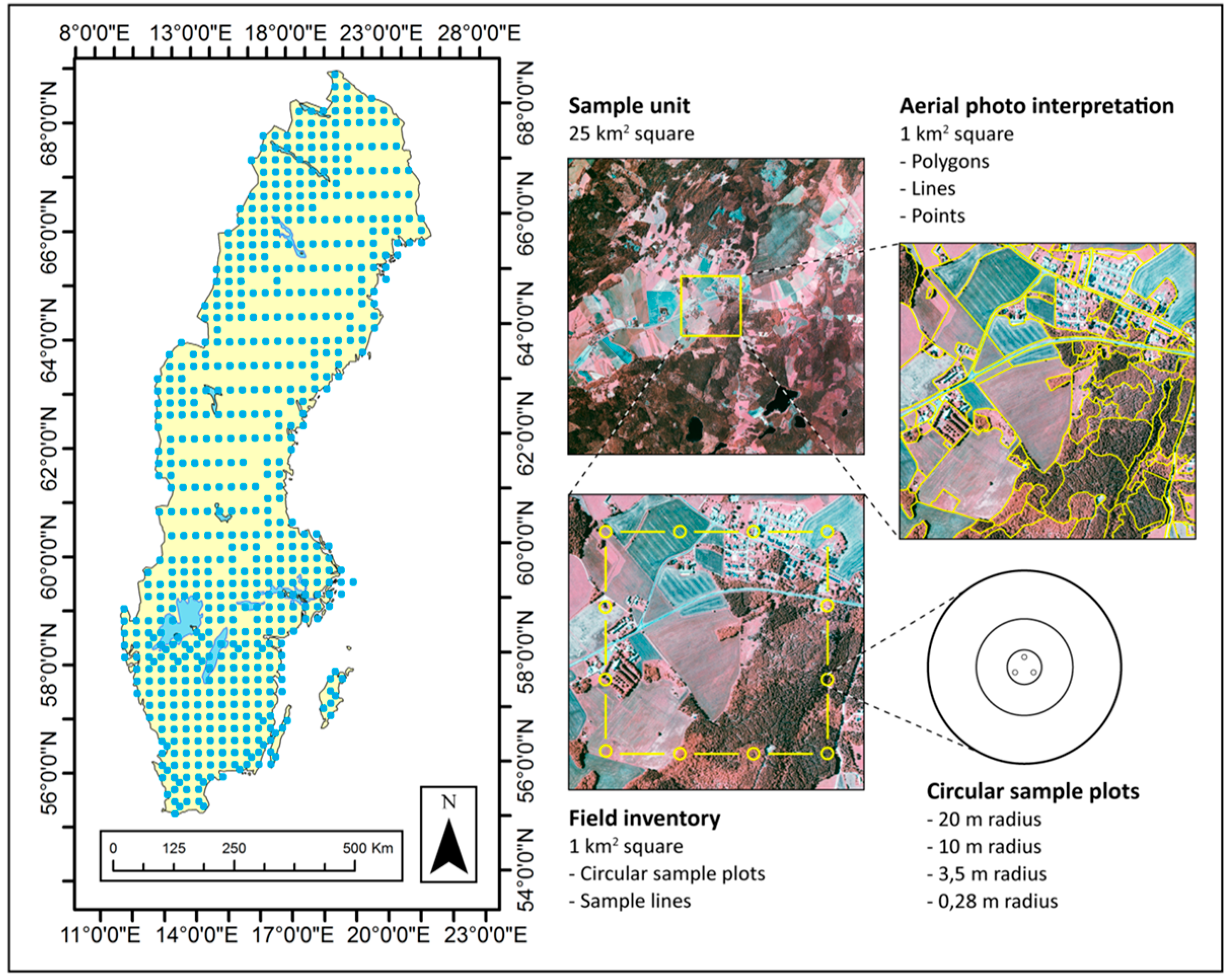
NILS data are collected from a stratified sample of 631 clusters. Each cluster contains 12 field surveyed sample plots within a 1 × 1 km square that is photo interpreted. Data interpreted include tree height; canopy cover above 3 m; canopy cover of bushes and small trees below 3 m; ground vegetation classes, and many more variables, for example, site moisture, tree species, spatial distribution of trees (clustered or spread out), coverage of water vegetation, aiming to describe the potential for biodiversity. The 1 × 1 km square is surrounded by a 5 × 5 km square (Figure 1). This larger square has so far mainly been used as a sampling frame for special inventories. The original ambition was, however, to also do a photo interpretation of the 5 × 5 km square, in order to obtain data that could be used for providing the landscape context to the data collected in the field and in the inner square. Visual interpretation of the 5 × 5 km squares has however proved to be too time consuming and thus costly. There is therefore a need to evaluate more automated and cost efficient methods for mapping the nationwide sample of the 5 × 5 km squares. One potential data source is optical imagery from earth observation satellites such as SPOT or Landsat, which have been much used for land cover classifications in the past [4,5,6,7,8].

Figure 1. Illustration of the National Inventory of Landscapes in Sweden (NILS) design. The 631 clusters are systematically sampled with different densities in 10 different strata. For each cluster 12 sample plots are visited in situ and a central 1 × 1 km square is photo interpreted. An outer 5 × 5 km square is supposed to contribute with data about the surrounding landscape. No coordinates are shown here as the position of individual NILS squares are confidential to assure that the permanent sample sites are not intentionally tampered with in any way.

Figure 1. Illustration of the National Inventory of Landscapes in Sweden (NILS) design. The 631 clusters are systematically sampled with different densities in 10 different strata. For each cluster 12 sample plots are visited in situ and a central 1 × 1 km square is photo interpreted. An outer 5 × 5 km square is supposed to contribute with data about the surrounding landscape. No coordinates are shown here as the position of individual NILS squares are confidential to assure that the permanent sample sites are not intentionally tampered with in any way.

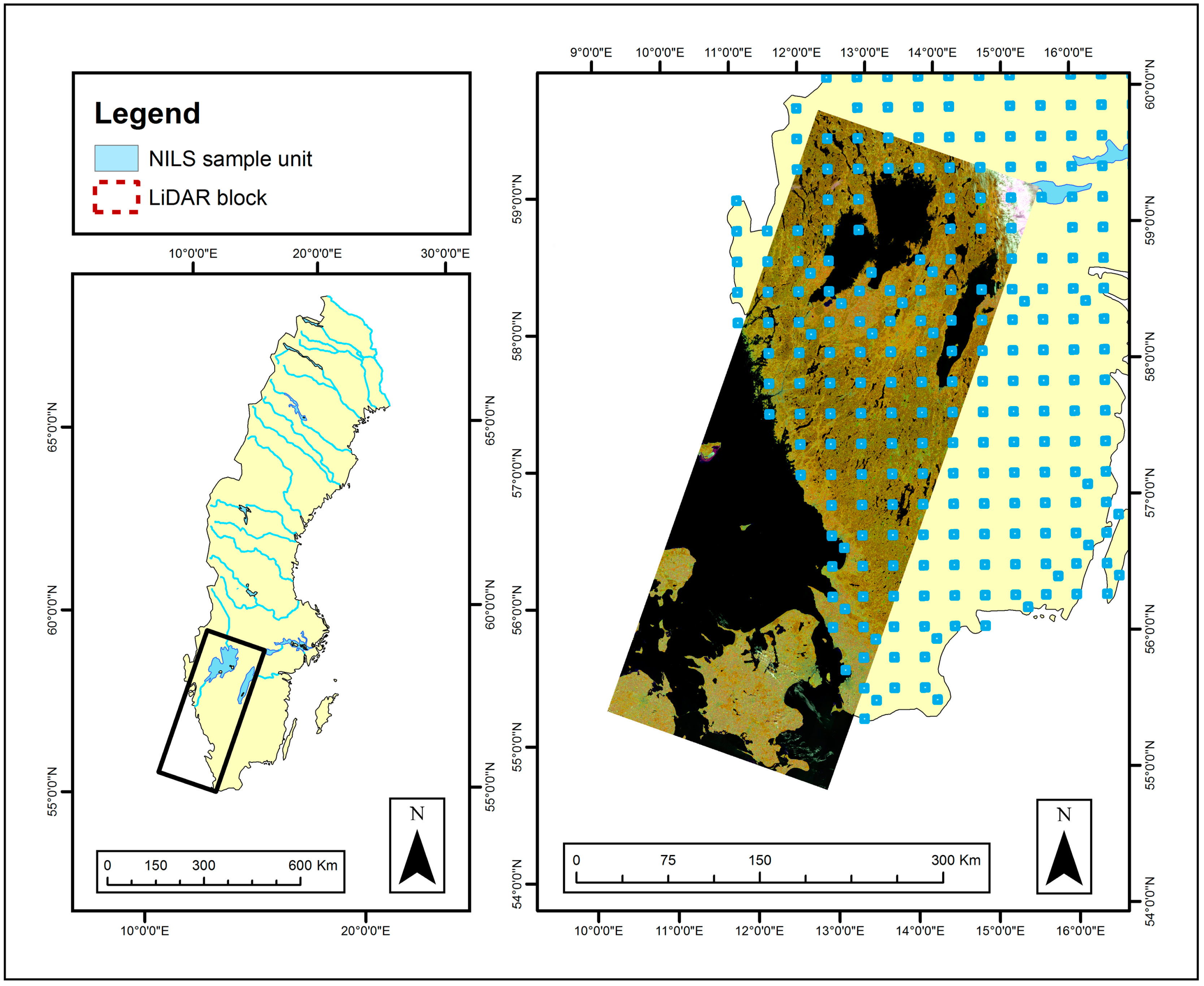
A nationwide scanning with airborne lidar is currently being carried out in Sweden [9]. Although primarily collected for the purpose of constructing a new national terrain model (or digital elevation model; DEM), the collected lidar data is also used by SLU on behalf of the Swedish Forest Agency for constructing a nationwide forest database [10]. Furthermore, it has been shown in earlier studies that lidar data is an excellent complement to optical satellite data for land cover classification, especially for the characterization of tree vegetation [11,12].

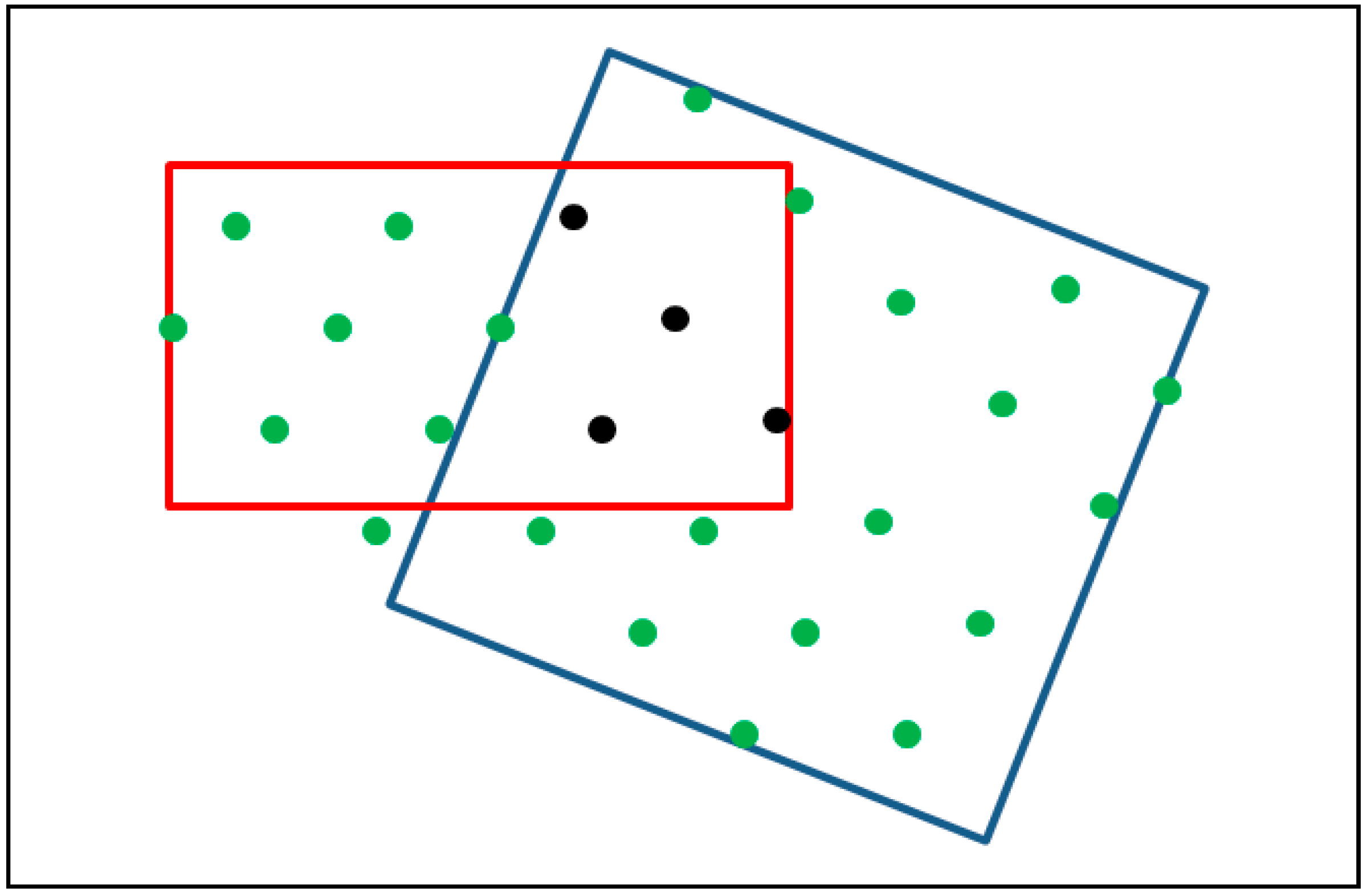
In order to minimize the need for new field reference plots, existing plots should be used as much as possible; in order to obtain enough plots as reference data, gathering plot data over large areas must often be done. It has been demonstrated in previous studies that metrics derived from different lidar scanners, and acquisitions from seasons may have differing properties [13,14]. However, the areas where satellite data have been acquired under homogeneous conditions (same sensor, acquisition date and atmospheric conditions) which overlap with lidar data acquired under homogenous conditions (e.g., same scanner and season) tends to be too small for obtaining enough existing ground reference plots (Figure 2). It may, therefore, be necessary to investigate a stratified approach where laser scanner data are used first for estimation of canopy cover and tree height, and then satellite data are used for classification of vegetation types within different the strata defined from the laser data based predictions.

Figure 2. Schematic illustration of the stratified approach for best utilization of existing field data and remote sensing data in large area operational studies. The blue rectangle represents a satellite data scene, the red rectangle is the area with laser scanner data acquired with the same sensor and during the same season and the dots represent clusters with existing field reference plots. When the lidar and satellite data are analyzed together, the plots marked in black show the field reference plots that could be used, whereas all plots covered by the respective data sets (black and green) could be used in the stratified approach where the data sets are analyzed in sequence.

Figure 2. Schematic illustration of the stratified approach for best utilization of existing field data and remote sensing data in large area operational studies. The blue rectangle represents a satellite data scene, the red rectangle is the area with laser scanner data acquired with the same sensor and during the same season and the dots represent clusters with existing field reference plots. When the lidar and satellite data are analyzed together, the plots marked in black show the field reference plots that could be used, whereas all plots covered by the respective data sets (black and green) could be used in the stratified approach where the data sets are analyzed in sequence.

The aim of the present study is to develop and evaluate a cost efficient method for semi-automated mapping of the nationwide sample (n = 631) of NILS 5 × 5 km squares by using the combination of airborne lidar data and optical satellite data (Landsat 8 and SPOT 5). Variables of interest are height and coverage of trees and bushes as well as broad vegetation types such as graminoids, dwarf shrubs and ground lichen dominated areas. Among the factors that need to be handled in this study are that different satellite scenes usually have an individual radiometric scaling and that the national set of lidar data are acquired with different scanners and during different seasons. Furthermore, in order to make upscaling to the national level economically feasible, existing field data should be used as much as possible and additional manual collection of reference data must be kept to a minimum. Thus, for classification of a given grid cell, reference data must be acquired either in the often limited area where both the used data sets overlap, or in a sequence, using a stratified approach.

2. Material

2.1. Study Area

The study area is located in the southwest of Sweden and is defined by three contiguous Landsat 8 Operational Land Imager (OLI) scenes acquired on the 23 July 2013 (Figure 3). This is done to simulate the approximate area covered by a future scene from the upcoming Sentinel-2 satellite which will have a scene size of 290 km by 290 km [15]. The area is large enough to contain various types of landscapes, such as coastal areas, and areas dominated by forest or agriculture. The forest is mainly dominated by managed coniferous forest of Norway spruce (Picea abies) the second frequent species is Scots Pine (Pinus sylvestris), but areas with broadleaved species forest are also present and of interest for biodiversity. In the open landscape ploughed fields dominate, and less intensively exploited open land is less frequent.

Figure 3. The study area in southwestern Sweden, defined by the extent of three contiguous Landsat 8 images. The lidar blocks are marked in red and the NILS squares are marked in blue.

Figure 3. The study area in southwestern Sweden, defined by the extent of three contiguous Landsat 8 images. The lidar blocks are marked in red and the NILS squares are marked in blue.

There are 106 NILS squares partly or completely within the Landsat scenes, of which two consisted of only a small proportion of land and were therefore not included in study. After removing NILS 5 × 5 km squares not completely covered by the Landsat scenes (5 squares), squares covered by clouds in the Landsat scenes (7 squares), squares scanned with more than one type of laser scanner, and squares acquired during different seasons or the laser data not delivered yet (22 squares), 68 squares remained. The above mentioned special cases (36 squares) will need to be handled in a future operational phase, but were left out during the method development phase.

2.2. Field Plots from the NFI and NILS within the Study Area

Two nationwide sample based inventories gather field plot data over the Swedish landscape: The Swedish National Forest Inventory (NFI) [16] and the National Inventory of the Landscapes in Sweden (NILS). The NFI plots are placed in rectangular clusters of two types: permanent clusters with 10 m radius plots revisited every 5 years and temporary clusters with 7 m radius plots. In total over 10,000 plots are surveyed annually by the NFI. While NILS focuses more on potential for biodiversity, the NFI is mainly focused on productive forests and does not cover the mountainous areas in the northwest of Sweden. An initial sample of 4117 NFI plots was selected from within the study area. Of these 2518 were temporary plots with 7 m radius and 1536 were permanent plots with 10 m radius and each tree positioned relative to the plot center. The coordinates for the center of the plots are positioned with GPS having about 1 m horizontal accuracy for most of the permanent plots and about 5 m horizontal accuracy for most of the temporary plots. The NFI is focused on obtaining measurements for trees, and could be used as field reference for tree height, canopy cover and tree species classification. Only a proportion of the permanent NFI plots contain detailed data about the field layer vegetation, with a total of 604 for the test area. In the open land, NFI plots with detailed ground vegetation data were available for only 22 mire plots. Thus, the NFI plots were considered suitable for estimation of canopy cover, tree height and classification of the forest strata, but not for classification of the open land strata.

The total number of NILS squares in the test area was 104, which in total contained 1248 plots. Some plots had however not been visited in the field, such as gardens and areas with growing crops. Furthermore, plots split by different types of land cover were not used, because the remote sensing signatures are expected to be a mix of different classes. Parts of the NILS squares in the area were also covered by clouds and had to be removed from the test. Possible training data left from NILS was then 587 plots of which 85 had canopy cover of less than 10% (from subjective field estimates). Plots on ploughed fields could not be used because of the rapid changes (i.e., seasonal planting and growth) of the vegetation. Clear-cuts are best mapped from multi-temporal images, which was done using visual interpretation as reference data. Plots on clear-felled areas were therefore not included as reference data. After removing clear-cuts and ploughed fields the total number of remaining plots suitable for use as reference data in the classification of open land was only 58, which was considered too limited a sample.

2.3. Satellite Data

The satellites scenes used in the project were geometrically precision corrected optical images from the Swedish satellite data archive SACCESS [17] (Table 1). No atmospheric correction to reflectance was done on the Landsat-8 images since the satellite data used were acquired on the same date. To perform change detection, histogram-matching of the SWIR band from the SPOT-5 scenes acquired on multiple date was used to account for radiometric differences. This was followed by subtraction of the earlier date image band from the later date and applying a threshold to detect clear-cuts.

Table 1. Satellite scenes used in the development project.

Satellite and Sensor	Path/Row	Date	Pixel Size	Used for
Landsat 8 OLI	195/19-21	2013 July 23	30 m	Tree species classification
SPOT 5 HRG	054/235	2005 June 29	10 m	Change detection
SPOT 5 HRG	053/234	2011 June 29	10 m	Open land classification and change detection

Table 1. Satellite scenes used in the development project.

Satellite and Sensor	Path/Row	Date	Pixel Size	Used for
Landsat 8 OLI	195/19-21	2013 July 23	30 m	Tree species classification
SPOT 5 HRG	054/235	2005 June 29	10 m	Change detection
SPOT 5 HRG	053/234	2011 June 29	10 m	Open land classification and change detection

2.4. Lidar Data

The lidar data used in the project were acquired by the Swedish National Land Survey [9], primarily for construction of a new national DEM. This national scanning started 2009 and is scheduled to conclude in 2015. The maximum scan angle is 20 degrees and the average number of return pulses is commonly around 0.7 returns per square meter. The scanning is done in blocks with the nominal size of 25 × 50 km. The aim (when possible) has been to scan each block with the same scanner, during as short a time period as possible. The different blocks are however acquired with different scanners and during different seasons and years. Most of the scannings in the study area were made with Leica scanners, but also Optech scanners were sometimes used. Within the study area there are 59 lidar scanning blocks, with the data being acquired mainly during 2010 and some during 2011 and 2012. Scanning during both leaf-on and leaf-off conditions and with different scanner types are present in the area.

In-house developed programs were used to pre-process the lidar point cloud. Scans from different flight strips overlap and only data from the strip with the lowest scanning angle were selected for each pixel. Height above ground was calculated for each point and the DEM created by the Swedish National Land Survey was used as ground references. The FUSION software [18] was used to compute metrics for the laser points above the ground elevation model for 12.5 m by 12.5 m grid cells. Metrics used were height percentiles and ratios of number of returns above a specified height.

2.5. Digital Aerial Photos and Map Masks

Sweden is being covered with digital aerial photos on a regular basis, with an average of every second year for Southern Sweden. Color infrared photos acquired by the Swedish National Land Survey [9] were used for interpretation of subjectively located training areas for open land. The photos were taken with the Z/I DMC camera at 4800 m above ground used, resulting in a pixel size of 0.5 m for the panchromatic band. In addition, map masks from the Swedish National Land Survey were used for delineation of urban areas and arable land. The map used was the Swedish property map, made for viewing at a scale of 1:10,000 showing detailed information of property borders and the landscape. The map masks were checked and adjusted by stereo air photo interpretation.

3. Methods

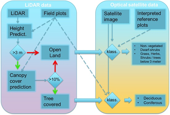
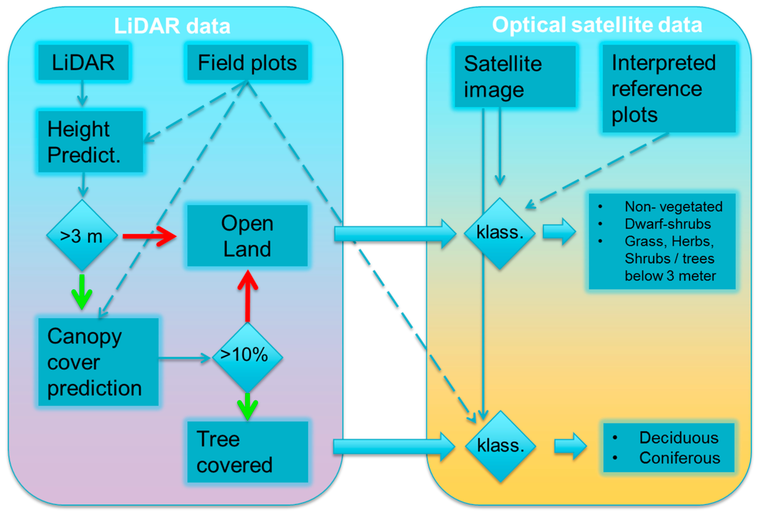
The method used for classification of the NILS square follows a stratified approach (Figure 4). Laser scanning data were used in a first stage to make predictions of height and canopy cover for laser scanning blocks. Predictions were then used to separate open land from tree-covered strata, then classify both separately using different training data sets.

Figure 4. Proposed workflow to classify a group of NILS 5 × 5 km squares. Left box contains the workflow for lidar predictions which uses only existing field data from NFI and NILS. Right box contains the workflow for predictions from optical satellite data. Red arrow indicates negative answers and green positive.

Figure 4. Proposed workflow to classify a group of NILS 5 × 5 km squares. Left box contains the workflow for lidar predictions which uses only existing field data from NFI and NILS. Right box contains the workflow for predictions from optical satellite data. Red arrow indicates negative answers and green positive.

3.1. Prediction of Tree Heights and Canopy Cover from Lidar Data Trained with NFI Field Plots

In the NILS design, mean tree height and canopy closure are key variables controlling workflow and variables acquired. The proposed automated workflow in the 5 × 5 km square follows the same structure. In NILS’ interpretation of the 1 × 1 km sample frame, canopy cover is defined as canopy cover ignoring within crown gaps, and tree height is defined as basal area weighted mean tree height. From the 59 lidar blocks within the test area all blocks that were scanned during more than one season or with more than one scanner brand or to a greater extent covered by clouds in the optical image were excluded from the analysis, leaving 41 blocks to predict. For each block, regression models for prediction of canopy closure and mean tree height were estimated using NFI plots as reference data and lidar metrics as independent variables. The aim was to gather at least 250 sample plots from the NFI for the training of each regression model. To cover a large enough area, adjacent blocks scanned in the same season (leaf-off or leaf-on season) with a scanner from the same manufacturer (Leica or Optech) were also used. Primarily, blocks within as near a distance as possible were selected, and the distance from the plots used to the center of the predicted block seldom exceeded 150 km. If the maximum distance exceeded 100 km, both permanent and temporary plots were used; otherwise, just permanent plots were used. From these selected blocks, plots which were field inventoried within a maximum of 5 years from each block’s scanning date were used to build the regression models. Forecast models for forest growth implemented in the Heureka forest planning system [19] were used to calculate the state of the forest at the respective year of the scanning for each plot.

Stem diameter to crown radius relationships using data from the NFI [20] were used together with known tree positions and stem diameters to calculate the proportion of canopy cover on the plots. The proportion of canopy cover was calculated on an inner 7 m radius circle to reduce effects of trees outside the plot with canopy reaching inside it. Small trees (<100 mm dbh) are measured on a smaller plot (3.5 m radius) in the NFI. Thus, the same density and diameter distribution of small trees in the 3.5 m radius plot was assigned to the full 10 m plot. Trees with stem diameter less than 40 mm are only calipered on two 1 m radius sub-plots within each NFI plot. The contribution to the total canopy cover from trees smaller than 40 mm in diameter was considered to be too small and was therefore not used. The method was then used for assigning canopy cover estimates to the NFI plots in the study area.

The canopy cover on the NFI plots is also subjectively estimated by the field personnel. Earlier results [21,22] show a good correlation with proportion of laser returns in the vegetation, and the subjectively estimated reference data were considered less accurate and therefore not used. Instead, the above described procedure with simulated canopy cover based on stem diameters and stem positions were used. Canopy cover and mean tree height for the 12.5 × 12.5 m raster cells within the NILS 5 × 5 km squares in the test area were then predicted using regression analysis.

Lidar data were extracted for each of the NFI plots in the test area. The FUSION software [18] was then used to calculate numerous metrics for each plot. Based on results from previous studies [21,22,23,24] a subset of these metrics was tried in regression analysis. The selected metrics were height percentiles and ratios of returns from vegetation above a specified threshold (vegetation ratios). The same explanatory metrics were selected for model use in all of the blocks, but regression parameters estimated for each block separately. The models of mean tree height used percentile 95 from laser data as an explanatory variable. Vegetation ratio over 1.5 m was chosen for all regressions predicting canopy cover. Vegetation ratios with different thresholds were tested, but because the difference among the ratios using different thresholds was very small selecting one threshold for all blocks seemed sufficient. Regression models were evaluated using leave-one-out cross-validation.

3.2. Classification within Tree Covered Stratum Using Optical Satellite Data

The lidar predictions of tree height and canopy cover were used to stratify the NILS 5 × 5 km squares in the test area into open land and forest areas, where forest was defined as having more than 10% canopy cover and trees over 3 m in height. Built up areas and arable land were separated from forests using map masks from the Swedish National Land Survey in some cases refined by visual interpretation in stereo color infrared aerial photos.

Within the forest stratum, a classification of tree species groups (broadleaved species or coniferous species dominated forest) was done, and for the open land stratum, a classification of ground vegetation was done. Each stratum was classified separately and with different sets of training data.

The tree species-group classification was trained with NFI plots for the whole test area. Plots above the defined thresholds of 10% canopy cover and 3 m tree height were used, and broadleaved vs. coniferous dominated forest was defined as having more than 50% of the total basal area on the plots of that particular class. The training data were first screened for outliers using scatterplots and visual interpretation of orthophotos. The total amount of plots left for classification, after obvious outliers like clear-felled forest and cloud covered areas had been removed, was 1186 of which 191 contained broadleaved species dominated forests.

The classification was done using the Random Forest algorithm, as implemented in the R statistical package [25]. The number of trees in the algorithm was set to 500 and the number of variables to try at each tree varied between 2 and 4. The imbalanced proportions of classes in the training data was handled by down sampling of the coniferous class, and final proportions were set to minimize the imbalance in the errors of omission and commission in the broadleaved species dominated class. No independent evaluation data were available, and because of the scarcity of broadleaved species forest in the training data, the data set could not be split into validation and training data sets. Therefore, the out of bag evaluation of error included in the Random Forest algorithm had to be used. Prediction of tree-species class was done for the 5 × 5 km squares in the test area.

3.3. Classification of the Open Land Stratum Using Optical Satellite Data

Based on the classes used in the manual interpretation of NILS 1 × 1 km squares, a classification system for the open land was developed based on spectral separability. The classes were non-vegetated; dwarf shrubs (mainly Erica spp and Vaccinium); grass/herb/bushes and/or small trees below 3 m; clear cuts; and water. The criterion for the classes were that they should have a dominance (>50%) of the respective vegetation class, except for dwarf shrubs which could be dominated by grass if only at least 25% was covered by dwarf shrubs. Clear cuts were defined as being cut during the last 5 years. Classification of open land was much more time consuming than classification of the tree covered stratum and was thus only tested for a subset of the NILS 5 × 5 km squares in the test area.

For the open land stratum, the availability of existing field plots available for use as reference data was considered to be too few to fully represent all vegetation classes. Stratification on open land would be sub-optimal for other aspects of the NFI or NILS inventory, thus a separate collection of field data for the open land stratum had to be done as part of the satellite image classification effort. Visual air photo interpretation in stereo of subjectively selected reference plots was used for the open land classification. The satellite data used in the test of the open land classification was SPOT 5 HRG images, resembling the spatial resolution of the upcoming Sentinel-2 satellite but having smaller scene extents. At least 10 reference plots for each class were subjectively selected. Each plot was 30 × 30 m, corresponding to nine SPOT 5 pixels.

Map information from the Swedish National Land Survey’s property map was aggregated into groups for the open land strata, such as lakes, arable land, built up areas, wetland, and other open land. Arable land and built up areas were masked from the satellite images and not classified. Some refinement of the map information had to be done using manual photo interpretation, for example, delineation of all built up areas and refinement of the open land was done. For the remainder of the open land stratum, maximum likelihood classification was used. The map stratum of wetland as well as that for other open land was classified separately as a way of incorporating map information into the classification.

Recent clear-cuts are of interest to map due to the different habitat quality they provide, and are best mapped using change detection with multi-temporal satellite images. This was tested using an older SPOT image over one of the test squares where open land classification was done. By subtracting the SWIR band from different images and applying a subjectively selected threshold to the difference, clear cuts and other changes were mapped. After eliminating changes occurring in fields and open wetlands, the remaining changed areas were assessed to be mainly clear-felled areas.

Finally, the classifications of forest and open land, as well as the areas excluded from classification and the detected clear-felled areas were combined for each evaluated NILS 5 × 5 km square. An independent validation of the open land classification was done for one of the NILS squares, using validation data collected by stereo photo interpretation. In this process, 200 plots were allocated systematically. If at least six of the nine SPOT pixels in the plot were of the same vegetation class, the plot was assigned that vegetation class.

4. Results

The accuracies of tree height predictions varied between 10.3% and 15.1%, measured as relative RMSE obtained by cross validation. Evaluations using independent data sets from other parts of Sweden where the same data and code have been used to produce tree height estimates show similar or slightly better results [10]. For heights below 3 m there was a tendency for the percentiles to be close to or at zero meters above ground.

Canopy cover estimates based on stem diameters and tree positions were evaluated for the detailed field material collected in [21]. The results for the test set of 28 plots were an RMSE of 8.2% and a positive bias of 3.9%. The lidar based predictions of canopy cover using NFI plots showed cross validation results between 19.9% and 28% relative RMSE. The worst accuracies were obtained from laser scanning blocks scanned during leaf-off conditions and with a large proportion of broadleaved species dominated plots in the training data. Scatterplots indicated an under-estimation of canopy cover for broadleaved species forest when the scanning was done during leaf-off condition.

The tree-species group classification showed good results. Users and producers accuracies from leave-one-out cross validation were found to be lower in the broadleaved species group as a result of the imbalanced reference data set (Table 2). The different balanced reference data sets showed different results and the sample of 350 coniferous and 170 broadleaved species dominated reference plots was the one with the most balanced errors of omission and commission for the broadleaved species class.

Table 2. Accuracy for Random Forest classification of broadleaved or coniferous species dominated forest in the tree covered stratum, using different independent variables and training data. Sat means optical satellite data, NDVI is Normalized Differential Vegetation Index, and Canopy Cover (CC) is predicted from cross validation in the regression models. The numbers in the variable combination column indicates the number of reference data plots (no. coniferous/no. broadleaved) drawn for each tree in Random Forest classification.

	User’s Accuracy (%)		Producer’s Accuracy (%)		Overall Accuracy (%)
Variable Combination:	Broadleaved forest	Coniferous forest	Broadleaved forest	Coniferous forest
Sat (300/150)	74	97	85	95	93
Sat (250/170)	71	98	89	93	92
Sat + NDVI (250/170)	71	98	88	93	92
Sat + CCpredicted (250/170)	72	98	89	93	93
Sat (350/170)	75	97	84	94	93
Sat + NDVI (350/170)	75	97	82	95	93
Sat + CCpredicted (350/170)	75	97	84	94	93

Table 2. Accuracy for Random Forest classification of broadleaved or coniferous species dominated forest in the tree covered stratum, using different independent variables and training data. Sat means optical satellite data, NDVI is Normalized Differential Vegetation Index, and Canopy Cover (CC) is predicted from cross validation in the regression models. The numbers in the variable combination column indicates the number of reference data plots (no. coniferous/no. broadleaved) drawn for each tree in Random Forest classification.

	User’s Accuracy (%)		Producer’s Accuracy (%)		Overall Accuracy (%)
Variable Combination:	Broadleaved forest	Coniferous forest	Broadleaved forest	Coniferous forest
Sat (300/150)	74	97	85	95	93
Sat (250/170)	71	98	89	93	92
Sat + NDVI (250/170)	71	98	88	93	92
Sat + CCpredicted (250/170)	72	98	89	93	93
Sat (350/170)	75	97	84	94	93
Sat + NDVI (350/170)	75	97	82	95	93
Sat + CCpredicted (350/170)	75	97	84	94	93

A confusion matrix for the classification of the open land stratum together with the tree covered stratum is shown in (Table 3). The tree covered stratum was included as one single class, for evaluation of the possible confusion between the different strata.

Table 3. Evaluation results for a NILS 5 × 5 km square. The tree covered stratum that was separated by threshold in lidar predictions of height and canopy cover is included as a single class.

Reference Data Class
Classification Result	Tree Covered Strata	Grass/Herbs/Shrubs	Dwarf Shrubs	Clear Cuts	Non-Vegetated	Water	Users Accuracy
Tree covered strata	73						100%
Grass/Herbs/Forbs/Shrubs	1	10					91%
Dwarf shrubs		3	11				79%
Clear cuts		1		4			80%
Non- vegetated					0
Water						5	100%
Producers accuracy	99%	71%	100%	100%		100%
Overall accuracy: 103/108 = 95%

Table 3. Evaluation results for a NILS 5 × 5 km square. The tree covered stratum that was separated by threshold in lidar predictions of height and canopy cover is included as a single class.

Reference Data Class
Classification Result	Tree Covered Strata	Grass/Herbs/Shrubs	Dwarf Shrubs	Clear Cuts	Non-Vegetated	Water	Users Accuracy
Tree covered strata	73						100%
Grass/Herbs/Forbs/Shrubs	1	10					91%
Dwarf shrubs		3	11				79%
Clear cuts		1		4			80%
Non- vegetated					0
Water						5	100%
Producers accuracy	99%	71%	100%	100%		100%
Overall accuracy: 103/108 = 95%

5. Discussion

In an operational inventory, cost and time consumption are main constraints to be considered; these are factors which are not always of importance in scientific studies for limited size study areas. By incorporating remote sensing, mapping of the NILS 5 × 5 km squares can be done efficiently. The most time-consuming task is then to gather reference data for the predictions, quality checking and correcting errors, and adding desired data that cannot yet be predicted automatically (for example land use information). The conclusion was that an efficient system had to be built, and as many resources as possible had to be saved for the time consuming yet important tasks of correcting errors and adding necessary additional data. In this project a main aim has therefore been to find existing suitable reference data. At first, the polygons from the NILS 1 km × 1 km squares were tested as training data. It was soon evident that the polygons were not suitable. A minimum mapping unit is used [26], and a portion of the polygons are therefore a mix of different classes causing confusing values in the remote sensing data.

The classification of open land classes showed good accuracies. Although the evaluation data set was very small, it gives an indication. In particular, the tree covered stratum increases the overall accuracy. The stratification into open land and tree covered strata were based on lidar data, which is well known for strength in characterizing the height and density of trees. The stratified approach with separate classifications of the open land and forest strata will allow classification of more classes than described in this paper. In the work done here, a few classes were selected in order to be more accurate and to reduce time consumption in gathering of training data. In the nationwide classification described in [5], a map mask was applied to Landsat data to separate forest from other cover types. The Landsat data in the forest stratum were then classified into coniferous, mixed and broadleaved species dominated forest as well as a number of forest classes based on height. NFI data were also used as reference data in this case, but the classification used spectral models and Maximum Likelihood with prior probabilities rather than the Random Forest algorithm used here. A stratification of forest and non-forest areas was also used in [27], and along with multi-seasonal satellite data, allowed more detailed tree species classification.

There is more information desired by stakeholders to be mapped in the NILS 5 × 5 km squares than can be predicted with the methods used here. Time series of previous remote sensing data can probably also provide information on the history of the different habitat, which in some cases can be important. Potential further development could, for example, be to map clear cuts from optical satellite data available from the 1970s and onward to provide some information on time since disturbance in the forest ecosystem [28].

An interesting phenomenon was found in forest covered pixels at the very edge of some lakes. The prediction of canopy cover was much higher compared to just one pixel further away from the lake. Some values were out of the range for the model and predicted over 100% canopy cover. These pixels were clearly over estimated, but no sufficient amount of evaluation data was available to fully investigate the effect. The effect was only present in some of the laser scanning blocks in the test area. After examining the point cloud a reasonable explanation was found. The point cloud lacked laser returns from the water surface, but not from the vegetation. When the canopy reaches out over the water, returns are registered from the vegetation only; the vegetation ratios were therefore higher than in the rest of the landscape given the same canopy cover. Since the border to water is of special interest for biodiversity and nature conservation, efforts were made to find ways to correct this but with little success.

An initial expectation was to be able to predict presence of lower-growing vegetation such as shrubs and small trees (below 3 m). The shrub/small tree cover from photo interpreted plots on subjectively selected sites in homogenous areas was compared to laser metrics. A very low correlation between presence of shrub/small trees and the laser metrics was found for all test sites, which was surprising given the good results in predicting canopy cover for taller trees. It should be kept in mind that the laser data were acquired with different scanners, and varying results may be due to the scanner that was used. It was seen that dense vegetation resulted in very few returns in the point cloud, giving vegetation ratios near zero. The reason for this might be that returns from low vegetation are mixed with the return from ground. Further studies that have used data from the Swedish national laser scan have shown similar results [10]. The lack of laser data at these lower heights is a likely influence on estimates for vegetation less than 3 m.

Over all, the experiences from this study showed that time efficiency in an operational classification system for a monitoring program like NILS is an essential component. The method developed here (Figure 4), where existing reference data are used as much as possible, seems to fulfill this.

It currently appears that the national laser scanning in Sweden is a one-time effort. NILS is an environmental monitoring program and needs updated predictions. Optical satellite data will be available and in particular Sentinel-2 data seem promising. The Swedish National Land Survey carries out aerial photography missions aiming to cover the entire country with two to six year intervals. During 2015 replacement of the lidar data with 3D point clouds from matched digital aerial photographs will be tested for estimates of height and canopy cover. Earlier studies where the use of photogrammetric point clouds has been evaluated show promising results for tree height predictions [29,30] but somewhat weaker results are expected for canopy cover and variables that depend on the density of the forest, such as basal area. In addition, in 2015, the earlier mentioned Sentinel-2 is expected to be launched, providing a new source of data that should be evaluated.