1. Introduction
Precipitation is a vital element of water cycle in the Earth System, which is closely related to ecological, hydrological, and meteorological processes [
1,
2]. Its spatial and temporal variations generally influence vegetation distribution, soil moisture and surface runoff [
3,
4]. Thus, high-quality of precipitation dataset is needed for the development of ecological and hydrological models at corresponding scales.
Precipitation dataset used in recent ecological and hydrological researches is mainly derived from three sources: (a) outputs from various numerical climate/weather models; (b) rain gauge observations; and (c) estimates from space-based observing systems [
5,
6,
7]. For example, the Global Climate Models (GCMs) can simulate the changes of precipitation at large scales [
5]; the Regional Climate Models (RCMs) can be used to predict the distribution of precipitation at a regional scale [
8]. Neither the GCMs nor the RCMs, however, can provide precipitation fields with higher spatial resolutions reflecting the spatio-temporal variations at small scales [
9]. Since the numerical weather models normally function at a coarse spatial resolution, scientists alternatively use
in situ rain gauge (spatially sparse) or satellite-based observations to build the precipitation dataset. With the help of spatial analysis technique, precipitation data from rain gauge stations can be interpolated and extrapolated over the regions with no data samplings. Daly [
10] has established a statistical regression model known as the Parameter elevation Regressions on Independent Slopes Model (PRISM) to simulate the distribution of precipitation over the Olympic Peninsula, in the northwest corner of Washington State, USA. The DAYMET model uses daily weather observations (1980–1997) to produce climate grids of annual total precipitation and other climatic variables over the continental US [
11]. Still, these rain gauge-based methods are accurate only within the area where rain gauge stations are spatially, densely installed [
12,
13]. Furthermore, weather radars offer an enormous potential to improve the quality of rainfall at high resolution. The wider spatial coverage of weather radars compared to that of a dense network of rain-gauges is an obvious advantage. However, despite the progress in technology and methodology over past decades, radar data are still not used as broadly and efficiently as they should be [
14,
15].
To acquire adequate and reliable spatial representations of precipitation over a broad area, scientists begin to explore novel approaches implementing the recent remote sensing precipitation products [
9,
14,
15,
16,
17,
18,
19]. The National Aeronautics and Space Administration (NASA) and the Japanese space agency (JAXA) launched the Tropical Rainfall Measuring Mission (TRMM) in 1997, which is one of the highest resolution products among all the current satellite precipitation datasets. TRMM has been extensively used for inter-disciplined investigations and applications, such as land surface modeling [
17,
20], climatic prediction [
21], and hydrological simulation [
22]. Nevertheless, the large pixel size (
i.e., 0.25°) of the TRMM precipitation data is too coarse for many regional and continental models, which generally need higher resolution inputs [
23]. The above precipitation products, thus, need to be, first, downscaled to meet the requirement of being in a high spatial resolution.
Statistical downscaling is a recently-developed approach in obtaining high spatial resolution of variables, based on conjugations between the variable at a coarse scale and geospatial predictors at a finer resolution [
24,
25]. This technique has been widely used for downscaling variables, such as land surface temperature [
26,
27], river flow [
28], soil moisture [
29,
30], and vegetation fraction cover [
31]. Specifically, studies of downscaling TRMM precipitation data have been conducted on at a regional scale in arid and humid regions. Fang
et al. [
32] assumed that the spatial variability of precipitation could be well explained by local topography and prestorm meteorological factors, and developed a statistical spatial downscaling scheme to disaggregate the TRMM 3B42 products into a 1 km gridded rainfall field in a mountainous area. An exponential statistical regression model between the Normalized Differential Vegetation Index (NDVI) and precipitation is useful to downscale precipitation from the TRMM monthly product in the Iberian Peninsula [
33]. Based on this downscaling method, Jia
et al. [
34] have developed a statistical regression model by introducing NDVI and elevation, which are seen as the main factors affecting precipitation, and have improved the resolution of the TRMM precipitation from 0.25° to 1 km in the Qaidam Basin. Similar to the examples above, two previous examples of downscaling research, Duan and Bastiaanssen [
24] used an integrated downscaling-calibration procedure of the TRMM 3B43 product with the limited rain gauge data sets to map monthly precipitation data at a higher spatial resolution (1 km) in humid and semi-arid regions.
Those previous approaches in recent literature can effectively downscale precipitation data at a local scale, but we need to explore the applicability of the existing algorithms for a larger spatial extent with complex terrain and different climate zones. Lovejoy
et al.’s [
35,
36] suggested global scaling of TRMM satellite radar data is quite remarkable, and extends from kilometers to the size of the Earth. Kang
et al. [
37] analyzed Next Generation Weather Radar rainfall data and found that rainfall fluctuations at spatial scales smaller than a reference scale exhibit self-similarity and that at scales larger than the reference scale, rainfall fluctuations are scale dependent. A coupled stochastic space-time intermittent random cascade model was then proposed to downscale summer daily rainfall for the Central United States from a scale of 256 km to a scale of 2 km. Chen
et al. [
38] assumed that the rainfall-geospatial factors relationship varies spatially but is similar in a region and constructed geographically weighted regression model for rainfall downscaling in North China. In addition, it is worth testing the validity of the suggested geospatial predictors (e.g., NDVI and elevation) because of certain contradictions in the literature: for instance, one analysis shows there is no clear relationship between precipitation and elevation in the Pangani Basin in Tanzania [
39], while another finds a clear relationship between them in the Qaidam Basin in China [
34]. Moreover, a number of geospatial predictors are still not explicitly examined in current research, and such predictors include geo-locations and topography (slope and aspect) that are associated with solar radiation and moisture conditions, in turn, granting significant impacts on precipitation [
40,
41,
42]. The analysis of the importance of predictors would be useful to investigate the potential of geospatial predictors with regard to downscaling precipitation over complex terrain and climate zones.
The Random Forest (RF) approach is an ensemble, purely statistically-based modeling, which constructs numerous small regression trees that vote on predictions using the random samplings of data and model layers [
43]. Amongst many non-parametric regression approaches, RF is receiving a considerable attention of ecological and other applications [
44,
45,
46]. This is because: (1) the robustness of RF may avoid over-fitting; (2) many different types of input variables can be implemented without variable deletion and regularization; and (3) it has tremendous analytical and operational flexibility. Thus, RF would be useful to build regression models for precipitation in relation to a number of geospatial predictors across different spatial scales, and to downscale the original TRMM 3B43 data to 1 km resolution.
In this study, our main goal is to investigate several downscaling approaches generating annual precipitation with a high spatial resolution over a variety of arid-humid regions in China Mainland. In this ultimate goal, three sub-objectives are: (1) to compare three statistical techniques (multiple linear regression, exponential regression, and RF regression trees) of modeling precipitation for better understanding how the model selection affects the performance of downscaling; (2) to explore the importance of input geospatial predictors in the regression models across different climatic zones; and (3) to generate the annual precipitation map of China mainland at a 1 km resolution, based on the best-performed downscaling approach. We fill the gap between the observation and estimates, and validate the final results with an independent precipitation dataset from 596 meteorological stations in China mainland. This research, in particular, demonstrates a unique application of machine learning technique (i.e., RF) to downscale the coarse TRMM 3B43 product, and, in turn, to provide a contextual framework for interpreting the fine spatial distribution of precipitation at a sub-continental scale. This study can have practical implications, particularly for biological researchers who require annual precipitation estimates at finer resolution as an input of tree height or biomass models over complex terrain, where they are characterized by the sparseness of in situ networks for precipitation measurement.
3. Dataset and Methodology
3.1. Dataset
3.1.1. Tropical Rainfall Measuring Mission
NASA and JAXA launched a joint project called the Tropical Rainfall Measuring Mission (TRMM) on 27 November 1997. TRMM aims to measure the intensity and area coverage of rainfall around the tropical and semi-tropical area where two thirds of the world’s rainfall happens [
50,
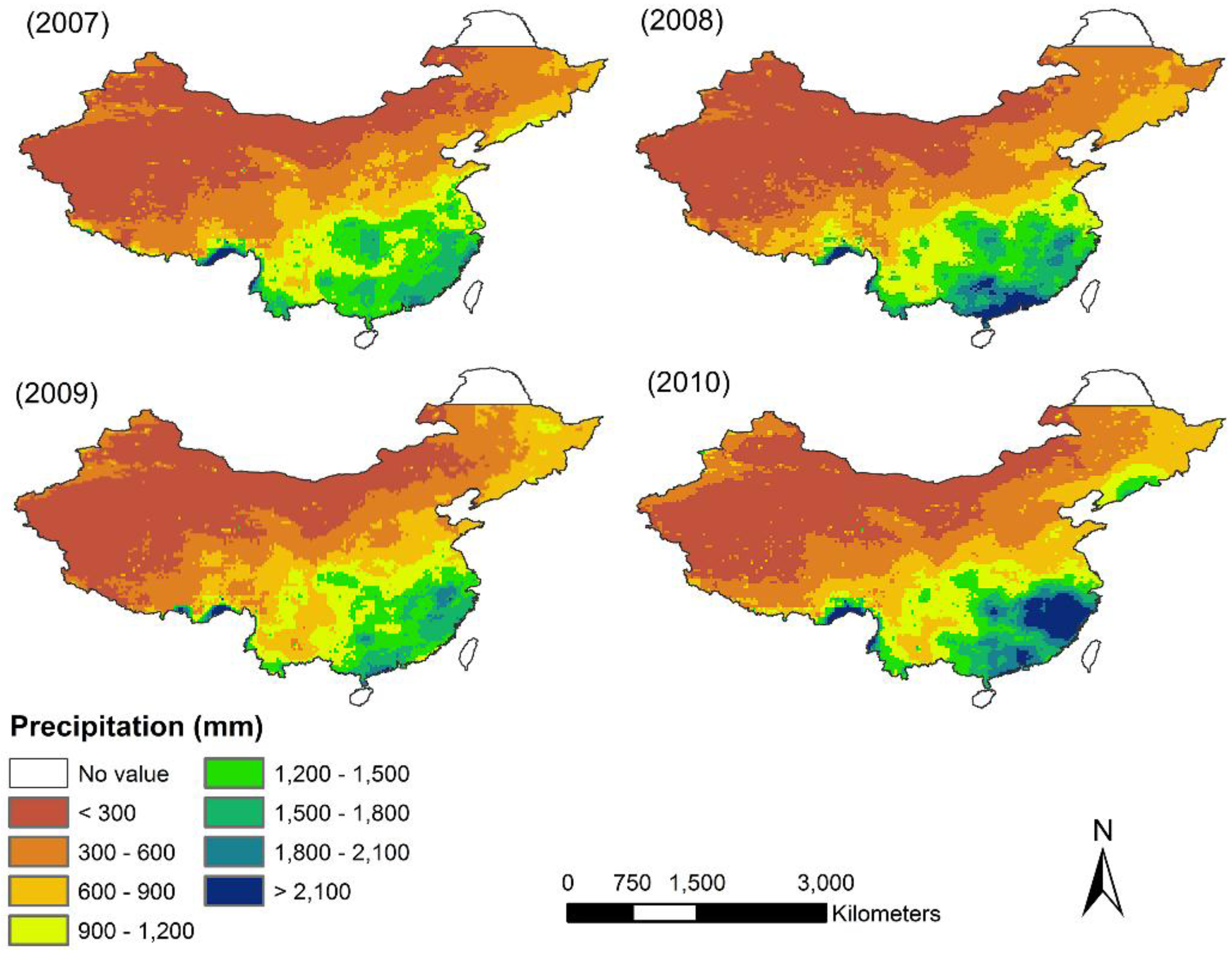
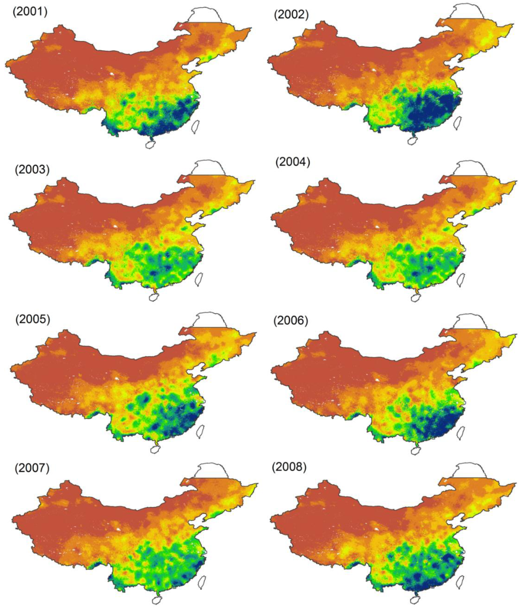
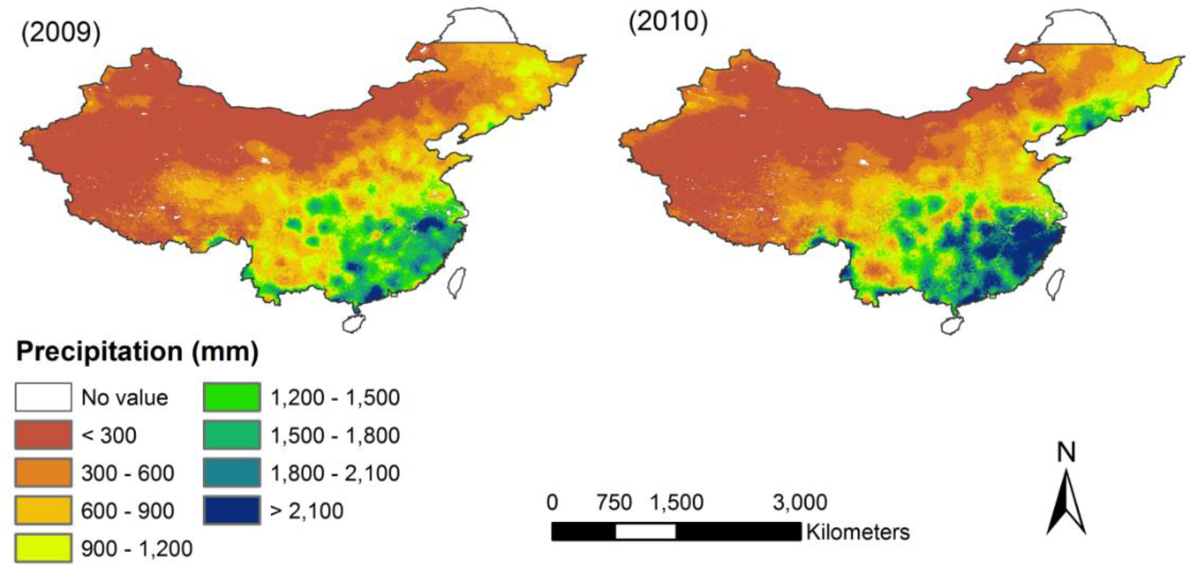
51]. TRMM can provide accurate precipitation data between latitude 50°N and latitude 50°S at the resolution of 0.25° × 0.25° (approx. 28 km × 28 km), which is high compared to other satellite-based products. There are two TRMM precipitation products commonly used, namely TRMM 3B42 and TRMM 3B43 datasets. TRMM 3B42 provides three-hour averaged precipitation values. It is converted into monthly TRMM 3B43 precipitation data, which was used in this study. We aggregated the TRMM 3B43 monthly product of Mainland China (12 months) into annual total precipitation of 2001 or 2010 at a spatial resolution of 0.25° (
Figure A1). The equation deriving annual total precipitation is as follows (Equation (1)):
where P
TRMM, i is the i-th annual precipitation of Mainland China from 2001 or 2010, P
TRMM_monthly, j is the monthly TRMM 3B43 precipitation product for j-th month (m = 12). The TRMM 3B43 dataset used in this study was provided by the International Scientific and Technical Data Mirror Site, Computer Network Information Center, Chinese Academy of Sciences (
http://www.gscloud.cn). The annual total precipitation in China from 2001 to 2010 is illustrated below (
Figure A1). We compared the scatterplots between annual rain gauge precipitation from rain gauge stations and the products from original annual TRMM 3B43 precipitation for 2001 and 2010 over Mainland China. We found original TRMM precipitation is in agreement with measured rain gauge data (R
2 = 0.92, RMSE = 176 mm, MAE = 108 mm, Bias = 0.05 for the year 2001, and R
2 = 0.94, RMSE = 157 mm, MAE = 52 mm, Bias = 0.06 for the year 2010).
3.1.2. Normalized Difference Vegetation Index
Based on differences in pigment absorption features in the red (~0.660 µm) and near-infrared (~0.860 µm) band, Rous
et al. (1974) proposed an vegetation index, called Normalized Distribution Vegetation Index (NDVI) [
52] (Equation (2)).
NDVI can be effective in responding to changes in the amount of green biomass, chlorophyll content, and canopy water stress, and have been widely used in various applications since it was proposed. Several investigations have indicated that there exists a strong positive correlation between precipitation and NDVI [
53,
54,
55]. In this study we chose the MODIS NDVI products as a geospatial predictor for the downscaling of TRMM precipitation. The characters of the MODIS NDVI products, MOD13A3, are listed in the
Table 1. We aggregated the MODIS monthly products, MOD13A3 (12 months), into the annual average NDVI of Mainland China for 2001 and 2010 at a spatial resolution of 250 m. We also generated the annual maximum, minimum, and range NDVI (maximum NDVI minus minimum NDVI) of Mainland China. Then, we resampled those products at a spatial resolution of 1 km by applying the nearest neighbor resize method. The equation deriving the annual average NDVI is as follows (Equation (3)):
where NDVI
avg.,i is the i-th annual average NDVI of Mainland China for 2001 to 2010, NDVI
monthly, j is the monthly maximum NDVI product for j-th month (
n = 12). We analyzed the NDVI trends during the research period and found the NDVI trends for all growing seasons increased moderately, except for NDVI values during the period of research years. This is consistent with the research conducted by Li
et al. [
56]. The MOD13A3 dataset used in this study is provided by the International Scientific and Technical Data Mirror Site, Computer Network Information Center, Chinese Academy of Sciences (
http://globalchange.nsdc.cn).
3.1.3. ASTER Global Digital Elevation Model
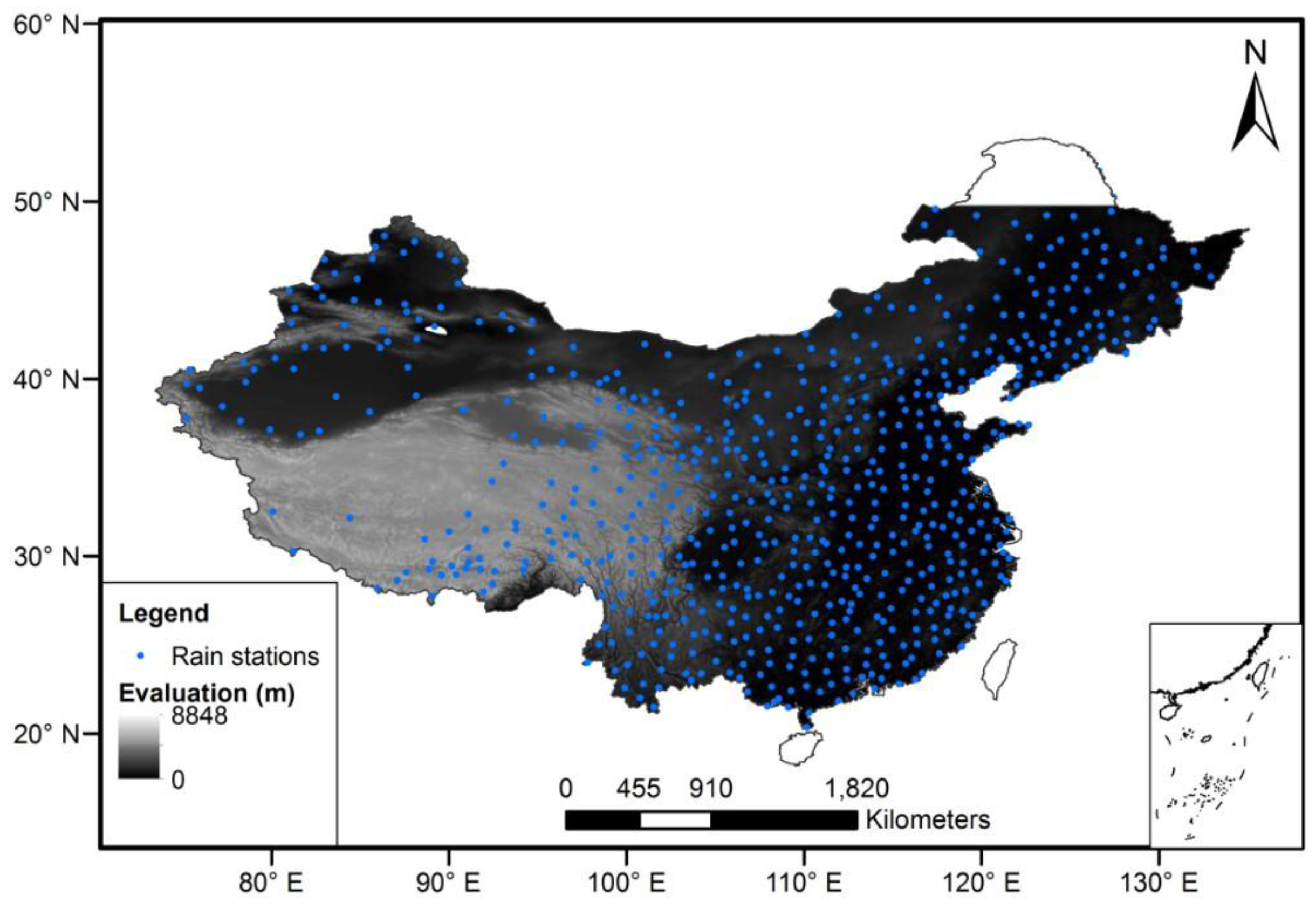
ASTER GDEM was released by the Ministry of Economy, Trade, and Industry (METI) of Japan and the United States National Aeronautics and Space Administration (NASA). ASTER GDEM covers land surface between latitude 83°N and 83°S of the Earth, which includes the entire area of Mainland China. GDEM version 2, with a resolution of one arc-second (roughly 30 m), was used in this study to analyze the influence of topography on precipitation (
Figure 1). In addition to the elevation data, two terrain attributions, slope and aspect, were derived from ASTER GDEM. The ASTER GDEM data was downloaded from the website,
http://gdem.ersdac.jspacesystems.or.jp/.
3.1.4. Rain Gauge Data
Monthly total precipitation datasets for 2001 and 2010 were used in this study to independently validate the final downscaled precipitation product. Those data were downloaded from the website,
http://cdc.cma.gov.cn. The precipitation values have been measured from 596 rain gauges of the national weather stations of Mainland China, which are distributed in a relatively sparse network. Most of the meteorological stations are mainly located in Eastern China, and few cover Western and Northwestern China (
Figure 1). Those monthly data were used to calculate the annual total precipitation of China over ten years. Our analysis indicates that the annual total precipitation for the period of 2001 and 2010 varied from 0 to 2672 mm/yr.
Table 1 lists datasets that were used in this study to build the statistical regression models and to downscale the precipitation.
Table 1.
Variables used in this study to construct the statistical regression models and to downscale the TRMM 3B43 precipitation product.
Table 1.
Variables used in this study to construct the statistical regression models and to downscale the TRMM 3B43 precipitation product.
| Variables | Dataset | Year | Resolution |
|---|
| Precipitation (mm) | TRMM3B43 | 2001, 2010 | Monthly, 0.25° |
| NDVI | MOD13A3 | 2001, 2010 | Monthly, 1000 m |
| Max_NDVI | MOD13A3 | 2001, 2010 | Annual, 1000 m |
| Min_NDVI | MOD13A3 | 2001, 2010 | Annual, 1000 m |
| Range_NDVI | MOD13A3 | 2001, 2010 | Annual, 1000 m |
| Elevation (m) | GDEM | 2010 | -, 30 m |
| Slope | GDEM | 2010 | -, 30 m |
| Aspect | GDEM | 2010 | -, 30 m |
| Latitude | - | - | -, - |
| Longitude | - | - | -, - |
3.2. Methodology
Statistical downscaling methods recently developed at regional scales were employed to downscale the TRMM dataset of Mainland China. The algorithms have successfully predicted variables at finer scales mainly based on the relationships between variables (such as land surface temperature and precipitation) and geospatial predictors (such as NDVI and elevation) [
24,
26,
34]. Commonly used regression models are the multiple linear and exponential models. The two models have generally performed well, using several combinations of different predictors at a regional scale in humid and arid areas. In addition to the above two regression models, RF may be also useful to construct the relationships between precipitation and geospatial predictors. In this study, we compared these three statistical techniques for modeling precipitation, and examined how the model selection affects the prediction accuracy (
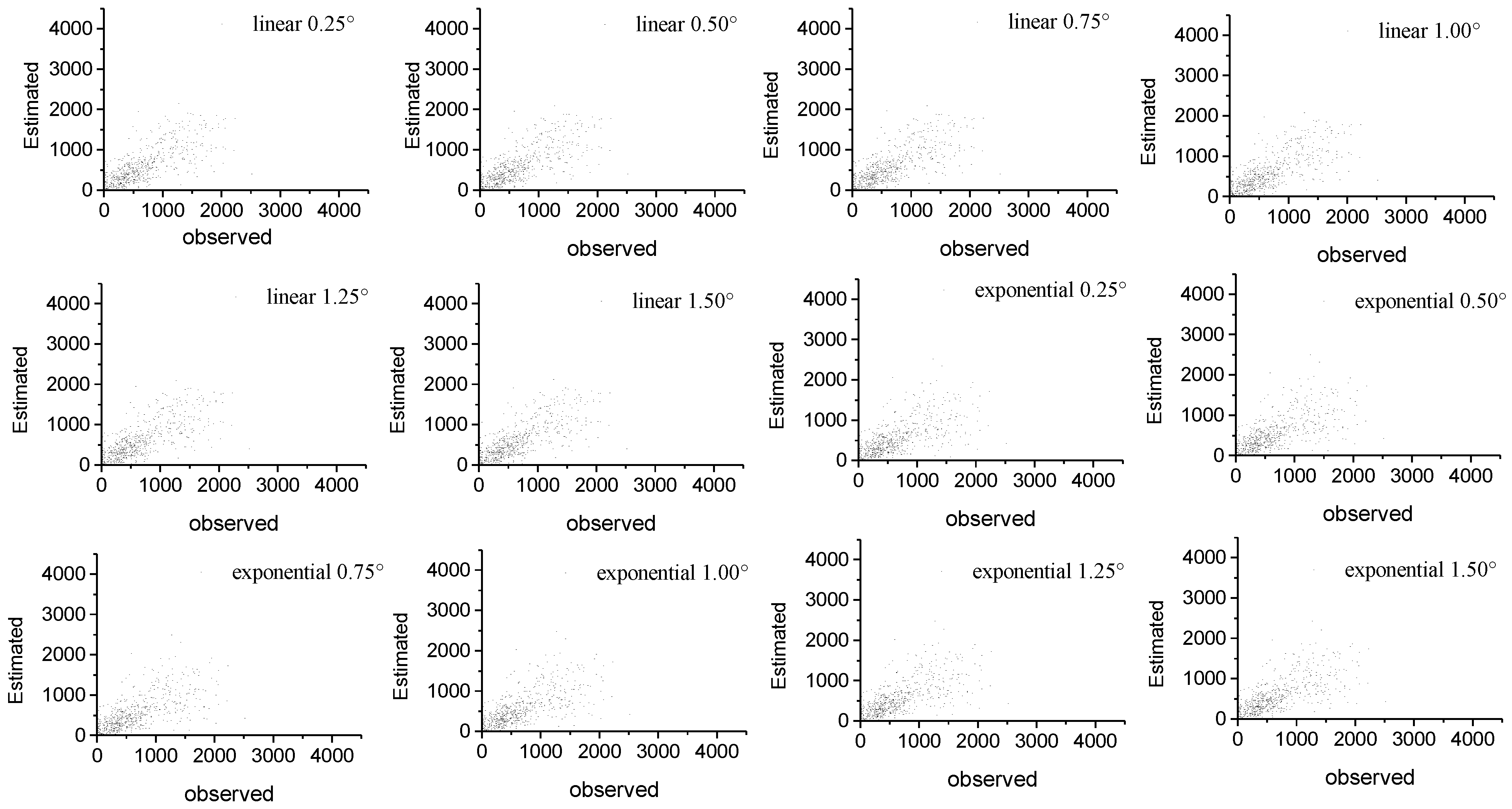
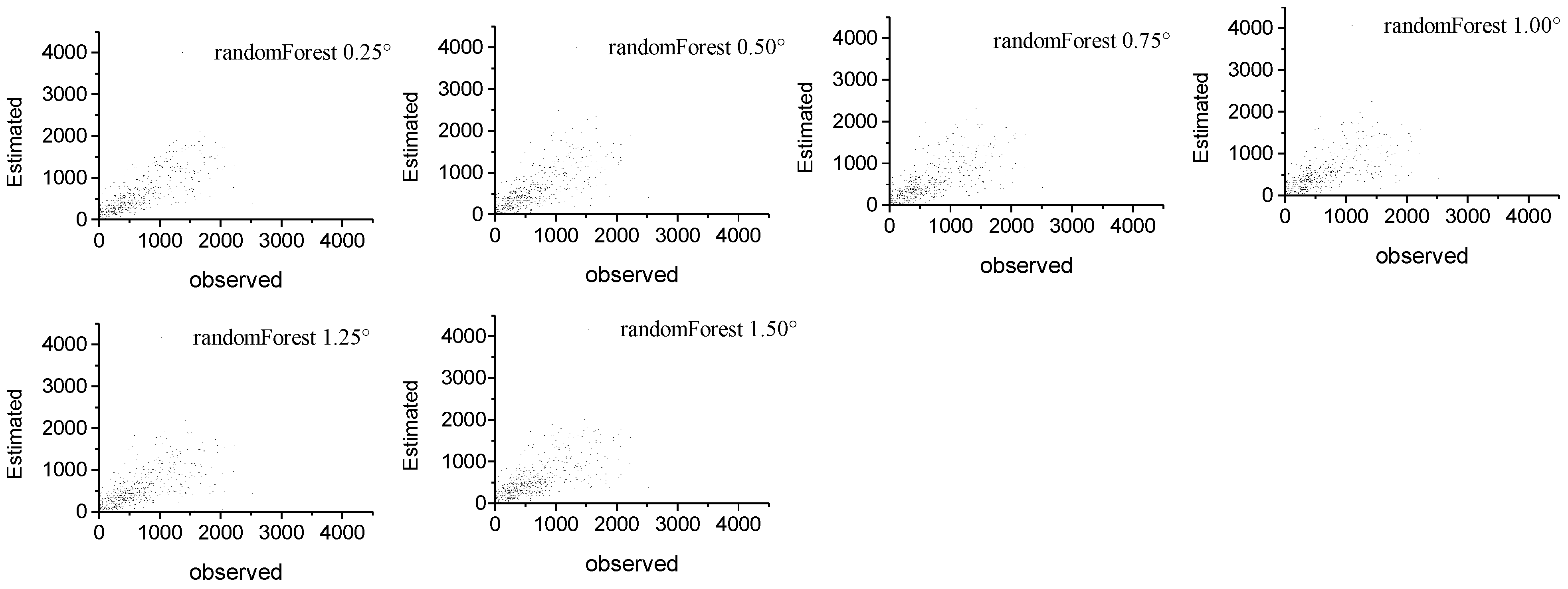
Figure A2,
Figure A3 and
Figure A4). Pre-processing has been used to model precipitation. The predictors have been centered and scaled, and transformed to a smaller sub-space with principal component analysis (PCA), where the new predictors are uncorrelated with one another. PCA transforming, centering and scaling of predictors were performed using in-house routines developed for R statistical software [
57,
58] and its caret package [
59]. Finally, the pre-processing progress changes the column names to PC1, PC2,
etc.
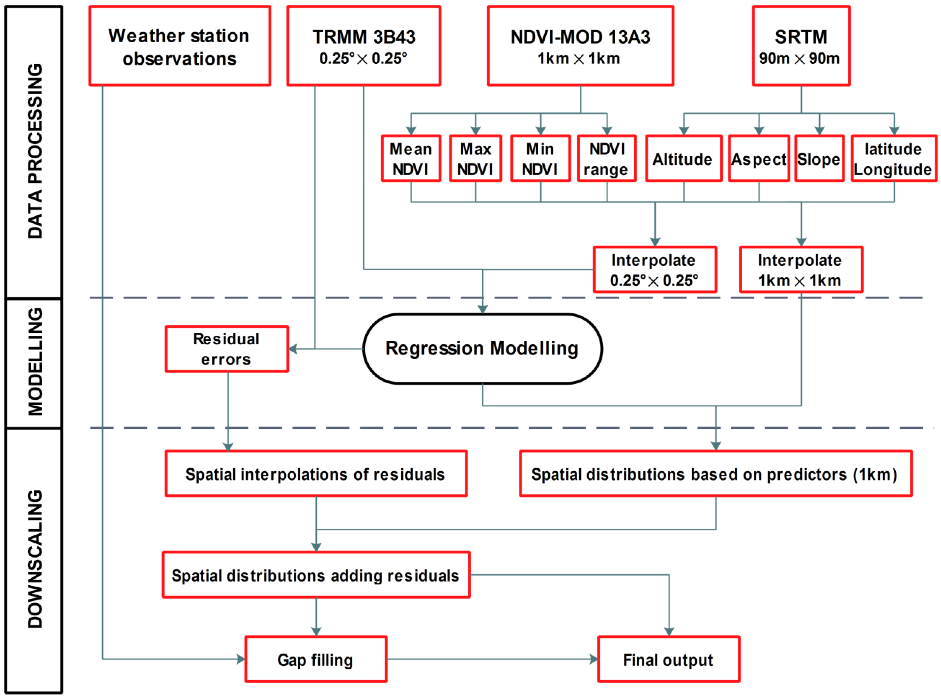
Similar to the processes proposed by Immerzeel [
33] and by Jia
et al. [
34], we designed the aggregation procedure in which several pre-processing steps also had to be carried out, as explained in the following section (
Figure 2).
Figure 2.
Flow chart of the downscaling algorithm used in the study.
Figure 2.
Flow chart of the downscaling algorithm used in the study.
(1) Pre-processing of the DEM and NDVI related datasets
Elevation, slope, and aspect at the 30 m resolution were extracted from the DEM of Mainland China and resized into a 1 km resolution by applying the pixel averaging technique. NDVI and NDVI related variables also are resized to a 1 km resolution by applying pixel averaging. Additionally, we extracted the annual average NDVI, annual maximum NDVI, annual minimum NDVI, and annual range of NDVI, TRMM 3B43-derived annual precipitation, elevation, slope, aspect, and latitude and longitude at 0.25° resolution by pixel averaging, respectively.
Regression modeling and prediction
Three statistical regression models (multiple linear, exponential, and RF) were then respectively constructed and tested at 0.25° scales. Here, independent predictors of the three models were annual average NDVI, annual maximum NDVI, annual minimum NDVI, annual range of NDVI, elevation, slope, aspect, latitude, and longitude. We then predicted the annual precipitation fields at a 1 km resolution by implementing the optimal coefficients of three statistical models to the geospatial predictors at a 1 km resolution (Pprt.).
(2) Generating final precipitation estimates
Part of the precipitation variability cannot be explained by the regression models. Those parts were generated by computing the difference between the predicted values at the 0.25° scale and the original TRMM 3B43, and then spatially interpolated into the residual (Pres.) maps at a 1 km resolution using a simple spline tense technique. Because of that, the residual data are regular-spaced and the spline technology is usually used for this type of data [
33], and the initial testing analysis shown that this kind interpolator performed better than other interpolators. The final precipitation estimates (P) of Mainland China at a 1 km resolution was obtained by adding the residual terms to the predicted terms (Equation (4)).
It should be noted that we excluded the precipitation values over water bodies and urban areas in the downscaling processes, because the three regression models generally produced no significant relationships between precipitation and geospatial predictors over water bodies and urban areas.
The gaps between final precipitation estimates (P) and measured precipitation at each rain gauge were filled by calculating the difference between them. The difference was summarized as follows [
24,
25,
60,
61]:
3.2.1. Linear Regression Model
Jia
et al. [
34] investigated valid relationships of precipitation with NDVI and elevation in a semi-arid area of Qilian Mountain, China, in the process of downscaling the TRMM 3B43 product. Similar to their work, we constructed multiple linear regression models at different scales and applied them to the downscaling process over the continental area of China. The regression linear model is written as follows (Equation (6)):
where a
1, a
2, …, a
n are the linear regression coefficients.
3.2.2. Exponential Regression Model
Immerzeel [
33] shows a strong coefficient of the correlation between NDVI and TRMM precipitation in Iberian Peninsula. Based on the Immerzeel’s method, we built an exponential regression model to downscale the TRMM 3B43 data of Mainland China (Equation (7)).
where a, b, c are the fitting coefficients of the regression model.
3.2.3. Random Forest Model
We employed RF to downscale the TRMM 3B43 precipitation at six different scales using geospatial predictors, including DEM, NDVI related variables, latitude, longitude, aspect, and slope at a 1 km resolution.
Random Forest (RF) is developed by Breiman [
43], based on the classification and regression trees (CART) algorithm. For regression in CART, vector Y represents the response values for each observation in variable matrix X [
19]. The matrix X and vector Y can be split into different subsets to regress a tree with a certain number of nodes. In each of the terminal nodes of the tree, a simple and accurate model is built to explain the relationship of X and Y. If the regression tree is built with sampled data, the tree then is able to predict another Y.
Splitting in regression trees is made in accordance with squared residuals minimization algorithm, which implies that expected sum variances for two resulting nodes should be minimized [
19] (Equation (8)).
where
,
are probabilities of left and right nodes;
,
are response vectors for corresponding left and right child nodes;
is optimal splitting satisfying the condition.
Averaging estimates is one way to reduce the variance of an estimate [
62] (Equation (9)).
where
is the m
th tree. This is called bagging [
43], which stands for the procedure of bootstrap aggregating.
However, simply re-running the same learning algorithm on different subsets of the data can result in highly correlated predictors. This may limit the amount of variance reduction that is possible. Thus, Breiman [
43] proposed a new technique called Random Forest (RF) to decorrelate the base predictors by learning trees on a randomly chosen subset of input variables.
The RF regression algorithm performs as follows [
63]: firstly,
ntree bootstrap samples X
i (i is bootstrap iteration) were randomly draw with replacement from the training dataset. The elements not included in X
i are referred to as out-of-bag data (OOB) for that bootstrap sample; then, for each bootstrap sample, an un-pruned regression tree was grown with the modification that at each node,
mtry of the predictors, were randomly sampled and the best split from among those variables chosen. Finally, new data (out-of-bag elements) were predicted by averaging predictions of the
ntree trees. The out-of-bag (OOB) samples in the training data were used to estimate prediction error, in which, the OOB samples were predicted by the respective trees and by aggregating the predictions. The out-of-bag (OOB) estimate of the error rate (ERROOB), were calculated as [
64]:
where
is the out-of-bag prediction observation i.
The orderings of the variable importance is an important issue in problems selecting variable by interpretation issues. The RF algorithm can also provide a measurement of variable importance by looking at how much the prediction error increases when left-out OOB data for that specific predictor variable is permuted while keeping the values of other predictors unchanged. These variable importance values are then used to rank orderings of those independent variables in term of their contributions to the regression model.
Here we used the R package of RF to model precipitation with geospatial predictors [
58]. Since precipitation is the continuous value, the RF regression tree approach was implemented in the study. We established “RF models” with the original TRMM 3B43 and other predictor data at six different scales in order to choose the best-performed RF model. In each RF model construction, the tree number of each “RF forest” was set as 500, and we conducted an iterative sampling process where each observation in the input dataset has an equal chance to be selected. A total of six geospatial predictors (NDVI, elevation, slope, aspect, latitude, and longitude) were used to grow “RF trees”.
In this study, the RF regression models were developed for both sub-regions and the entire study area. Annual precipitation at a 1 km resolution for the period 2001–2010, for the entire study area, was obtained by implementing the nation-wide RF model. On the other hand, we divided the whole study area into four zones: arid, semi-arid, semi-humid, and humid zones, depending on annual precipitation in the past regionalization studies of Mainland China [
65,
66]. The reasons for developing the sub-regional regression models were two-fold. First was to eliminate, as far as possible, the uncertainty caused by the nation-wide RF model when applied to each sub-region. The second reason was to analyze the importance of input predictor variables in the downscaling procedures across different regions.
3.3. Validation
Evaluations of the models and downscaling algorithms were divided into two parts: (a) the two-fold cross validation approach was implemented to investigate the performance of the three statistical models, respectively, and (b) the final downscaled precipitation products were validated by an independent precipitation dataset. The dataset provides the monthly precipitation measures from 596 meteorological stations over Mainland China in the period 2001–2010.
3.3.1. Two-Fold cross Validation
In the two-fold cross validation, we randomly divided the original input data into two sample sets at different scales. The first half data was used to train the models at each scale, while exploring the stability of model performances using the independent test sets (the second half data). For the purpose of model evaluations, we used the R
2 and RMSE. The R
2 between the modeled and TRMM estimates and RMSE at six different scales were calculated using Equations (11) and (12).
where O
i is the TRMM precipitation and P
i is the modeled precipitation of the i-th pixel, n is the total number of the TRMM precipitation pixel at each scale, and are the value of the TRMM precipitation and the modeled precipitation, respectively.
3.3.2. Validation with Ground Observations
The two-fold cross validation was only used to select the best-performed model at a certain scale to downscale the TRMM 3B43 precipitation. The accuracy of the final downscaled products should be further validated against the
in situ measurements from the rain gauge stations, based on the R
2, RMSE, mean absolute error (MAE), and bias. Here, we assume that the ground-measured precipitation could well represent the regional precipitation at a scale of 1 km. The MAE and bias were defined as follows (Equations (13) and (14)):
where O
i indicates the observed annual precipitation from the i-th rain gauge stations and P
i is the downscaled annual precipitation extracted at the location of the ith meteorological stations, n is the total number of the meteorological stations (
n = 596), and are the value of the observed and the downscaled precipitation, respectively. Several studies [
2,
3] demonstrated that the R
2 value is not enough to evaluate the prediction accuracy. Thus, in this study, we gave more weight to the MAE and bias in the evaluations.
4. Results and Validation
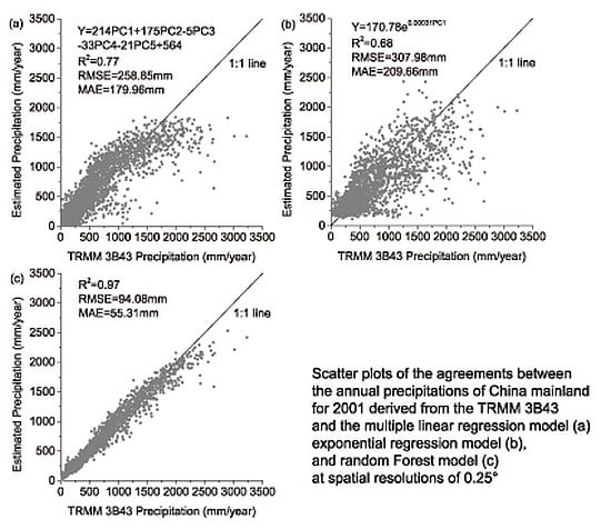
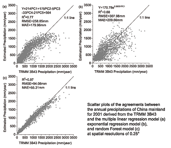
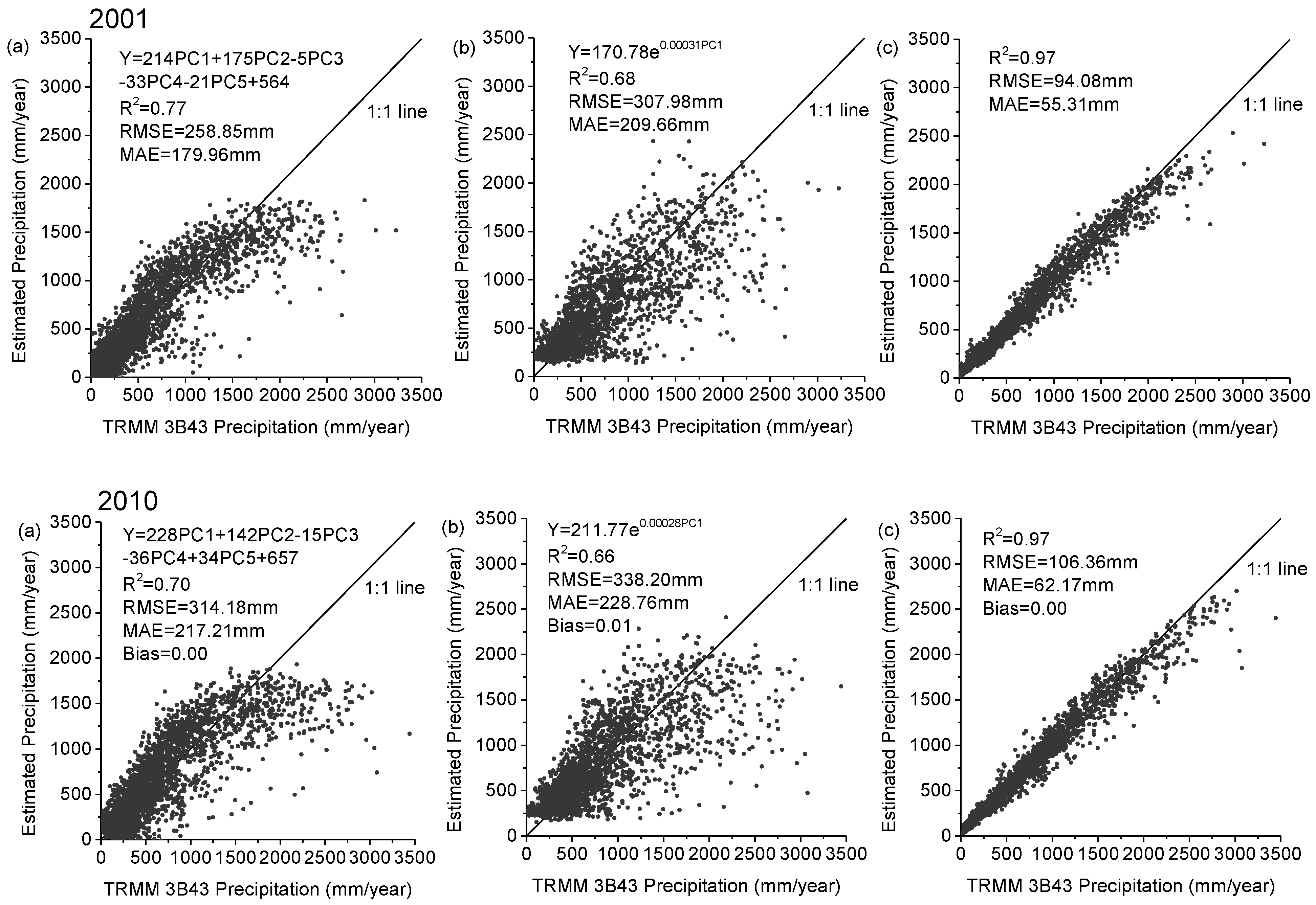
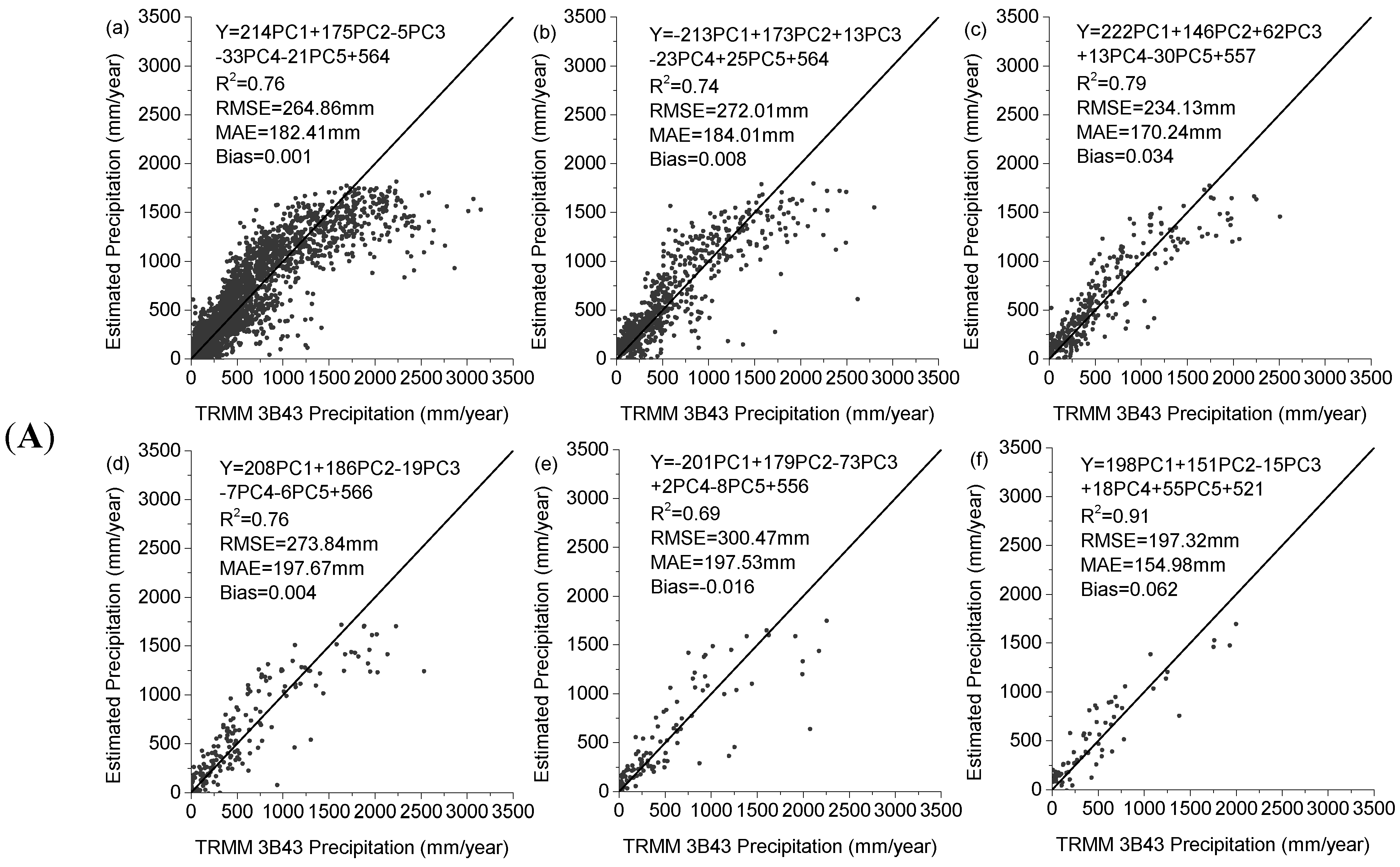
Figure 3 demonstrates the scatter diagrams for the annual precipitation derived from TRMM 3B43 and the predicted precipitation with the multiple linear, exponential, and RF models at 0.25° scale for 2001 and 2010. All the models qualified the significance test (all the
p values < 0.007 and all the R
2 > 0.66). However, for the linear model the underestimations were found where the TRMM precipitation was over 1200 mm/year in 2001 and 2010. For the remaining two models, the underestimations were also observed where the TRMM precipitation was over 2000 mm/yr in 2001 and 2010. All the models seem to dampen potential extremes; a possible reason is that the predictors used in the models, such as NDVI, elevation, are not so sensitive to the extreme rainfall. Extreme rainfall normally occurs in humid area; in this case, the NDVI value will not greatly change with increasing amounts of precipitation as vegetation can only absorb a certain amount of rain water. As shown in
Figure 3, the RF model performed best in terms of the R
2, RMSE, and MAE in 2001 and 2010, when compared to the two previous models.
Figure 3.
Scatter plots of the agreements between the annual precipitations of China mainland for the year of 2001 and 2010 derived from the TRMM 3B43 and (a) the multiple linear regression model, (b) exponential regression model, and (c) random Forest model at spatial resolutions of 0.25°, respectively.
The residual of the regression model was generated by subtracting the predictive value from the original TRMM 3B43, which represented the amount of precipitation that could not be explained by the regression model. The performance of the regress models, thus, would impact on the residual value. We calculated the relative weight of the predicted and residual rainfall fields in terms of the following equation:
The results for the three techniques are listed in the following table (
Table 2).
Table 2 implies the predicted rainfall derived with the RF method is very close to the final results. The addition of the residual term seems not to greatly improve the prediction accuracy of the results of the RF downscaling approach for the RF method. However, substantial residuals are found for the linear and exponential models, the ignorance of those residual values would finally reduce the accuracy of downscaling.
Table 2.
The relative weight of the predicted and residual annual rainfall fields for the three techniques for the year of 2001 and 2010 over Mainland China.
Table 2.
The relative weight of the predicted and residual annual rainfall fields for the three techniques for the year of 2001 and 2010 over Mainland China.
| | | Linear Regression | Exponential Regression | RF Regression |
|---|
| 2001 | RW_prd. | 2.16 | 3.44 | 1.14 |
| RW_res. | −1.17 | −2.44 | −0.14 |
| 2010 | RW_prd. | 2.14 | 2.01 | 1.07 |
| RW_res. | −1.14 | −1.01 | −0.07 |
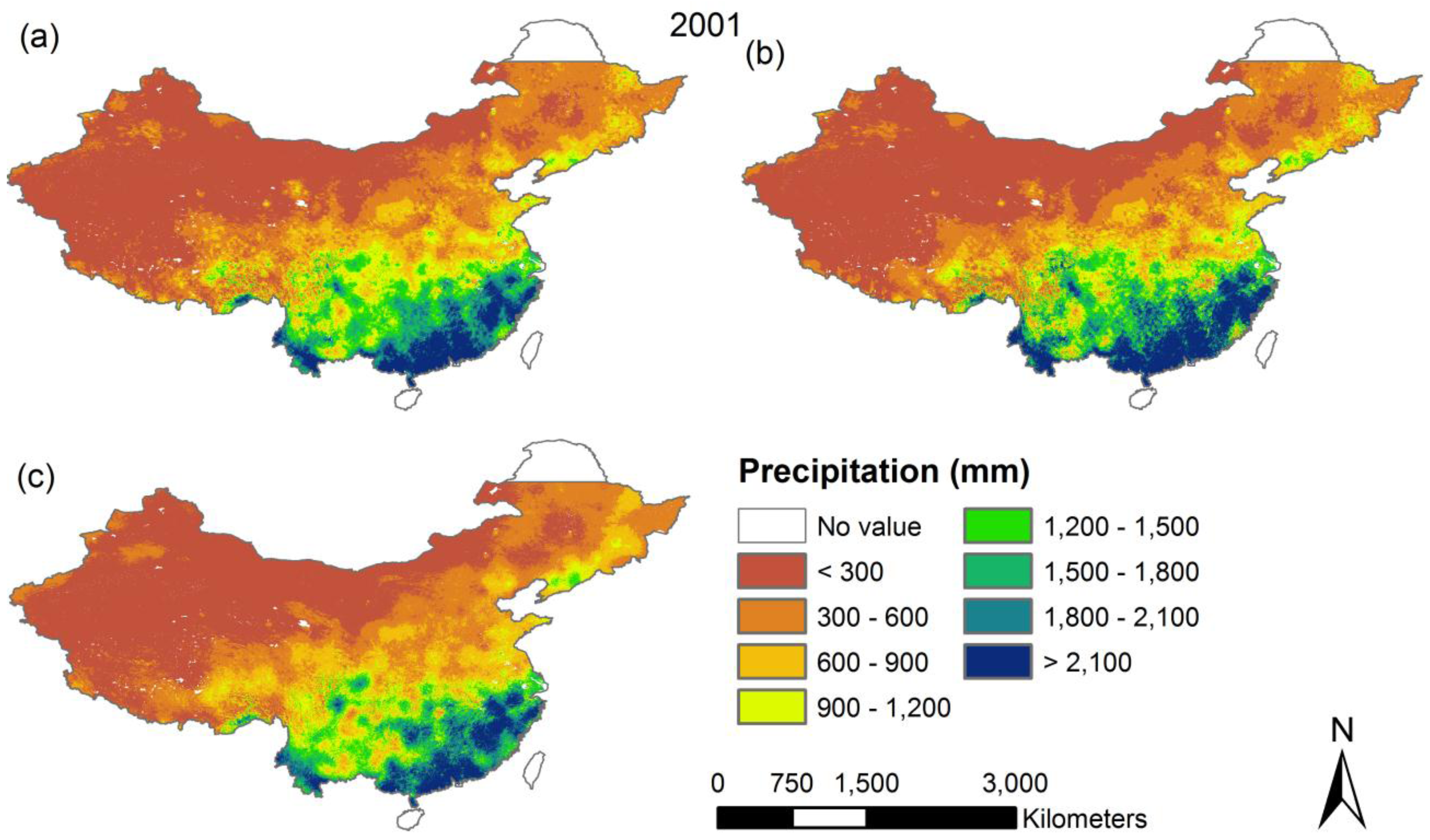
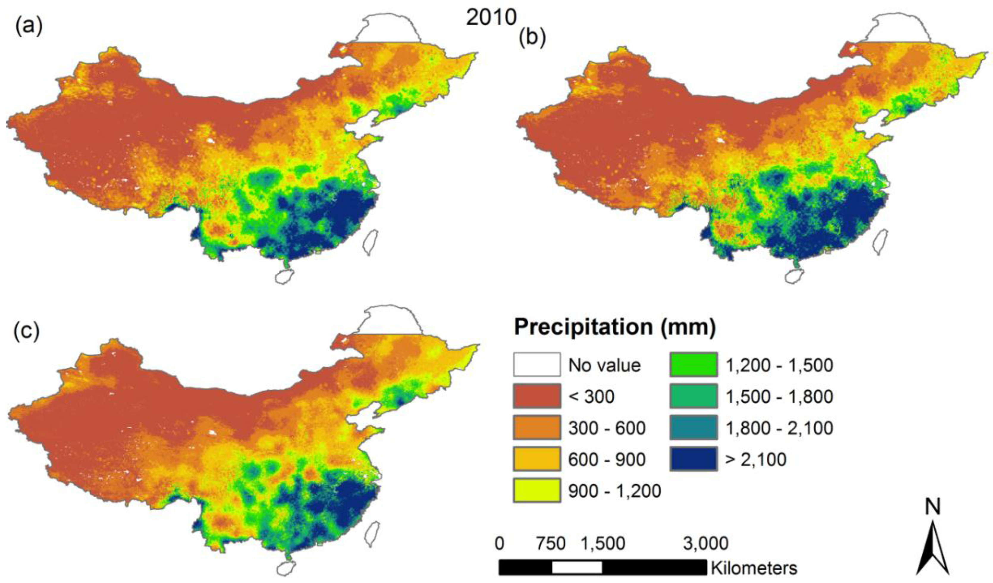
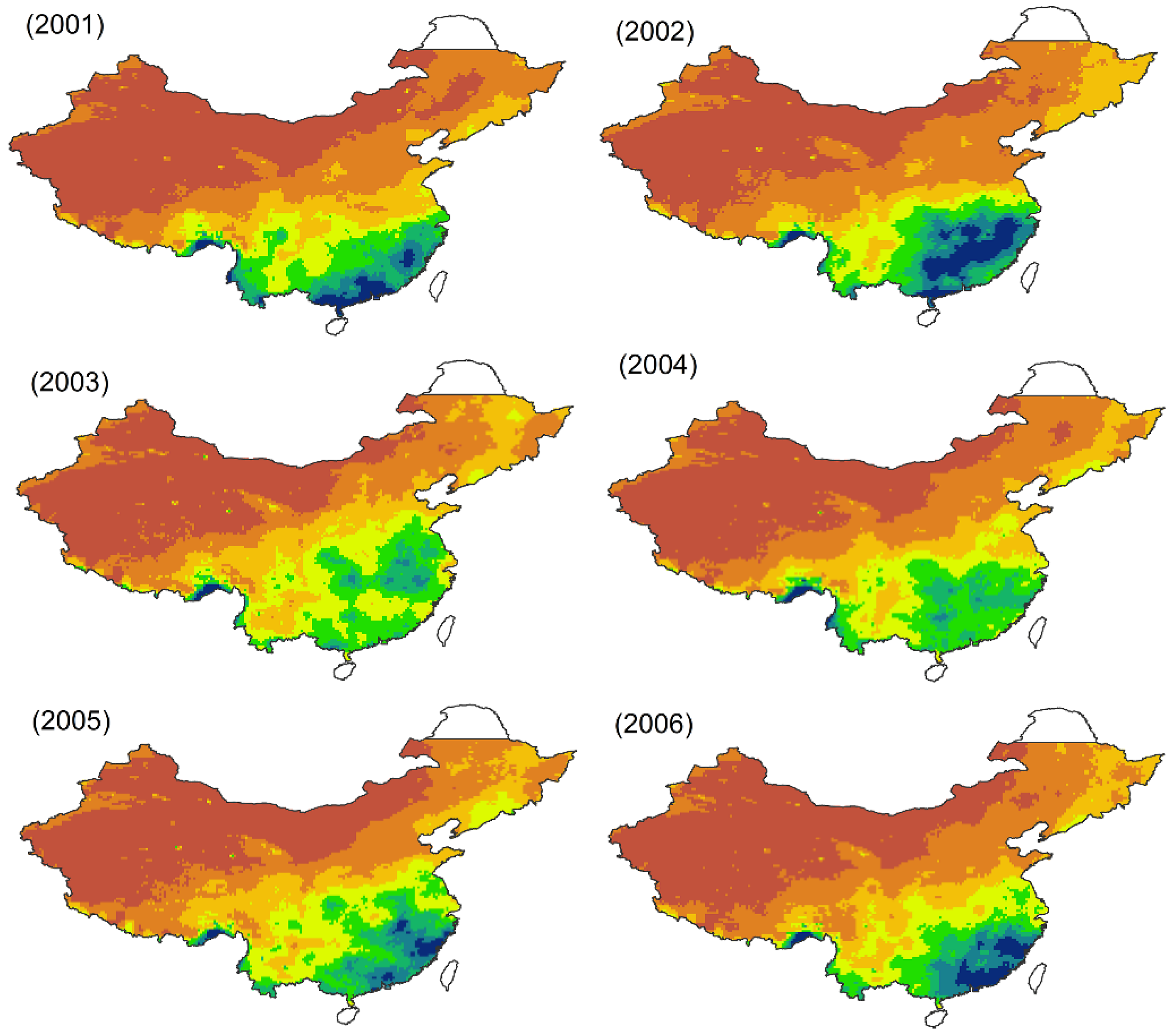
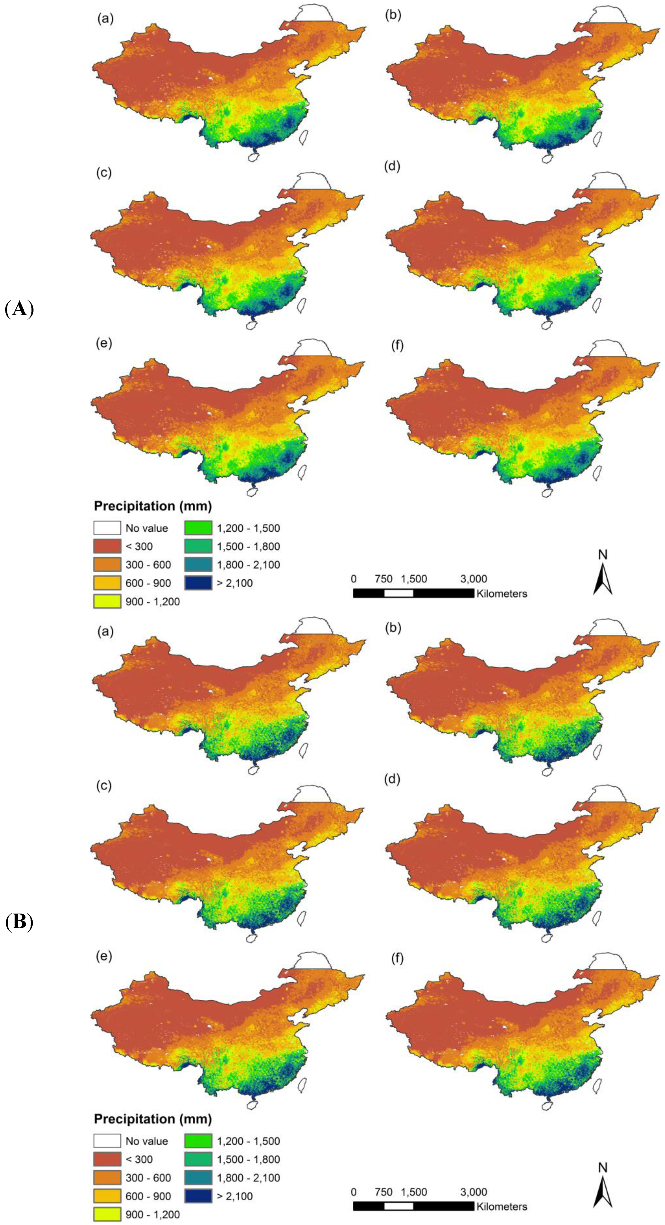
The three models’ coefficients were then employed to produce annual precipitation of Mainland China at a 1 km resolution. Here, we also produced the residual map at a 1 km resolution by interpolating residuals using a simple spline tension interpolator, which is the difference between the original TRMM 3B43 and the predicted precipitation at the resolution of 0.25°. The final downscaled product was obtained by combining the predicted values of annual precipitation and the residuals of precipitation at a 1 km resolution (
Figure 4). From the final map of downscaled precipitation derived from the three models, we noticed that the distribution of annual precipitation for the period of 2001 and 2010 over Mainland China reflects a strong gradient from the northwest to southeast.
Figure 4 reveals that in the wet year and dry year, the exponential method generates more extremes of high precipitation in humid areas, with a significantly larger standard deviation. The probable explanation for this is that the exponential method is markedly more sensitive to predictors of high value in humid areas. The RF method produces the least extremes of high precipitation. Furthermore, the RF downscaling product shows a smoothed pattern and did not present heterogeneous patches when compared to the final products derived from the other two models. The likely explanation is that many more decision trees built in the RF algorithm minimize changes in gradients, giving rise to smoother transitions in surface values across the research area.
Figure 4.
The final predicted annual precipitation of Mainland China at a 1 km resolution for the years of 2001 and 2010, using (a) the multiple linear; (b) exponential; (c) Random Forest and regression model, respectively.
Figure 4.
The final predicted annual precipitation of Mainland China at a 1 km resolution for the years of 2001 and 2010, using (a) the multiple linear; (b) exponential; (c) Random Forest and regression model, respectively.
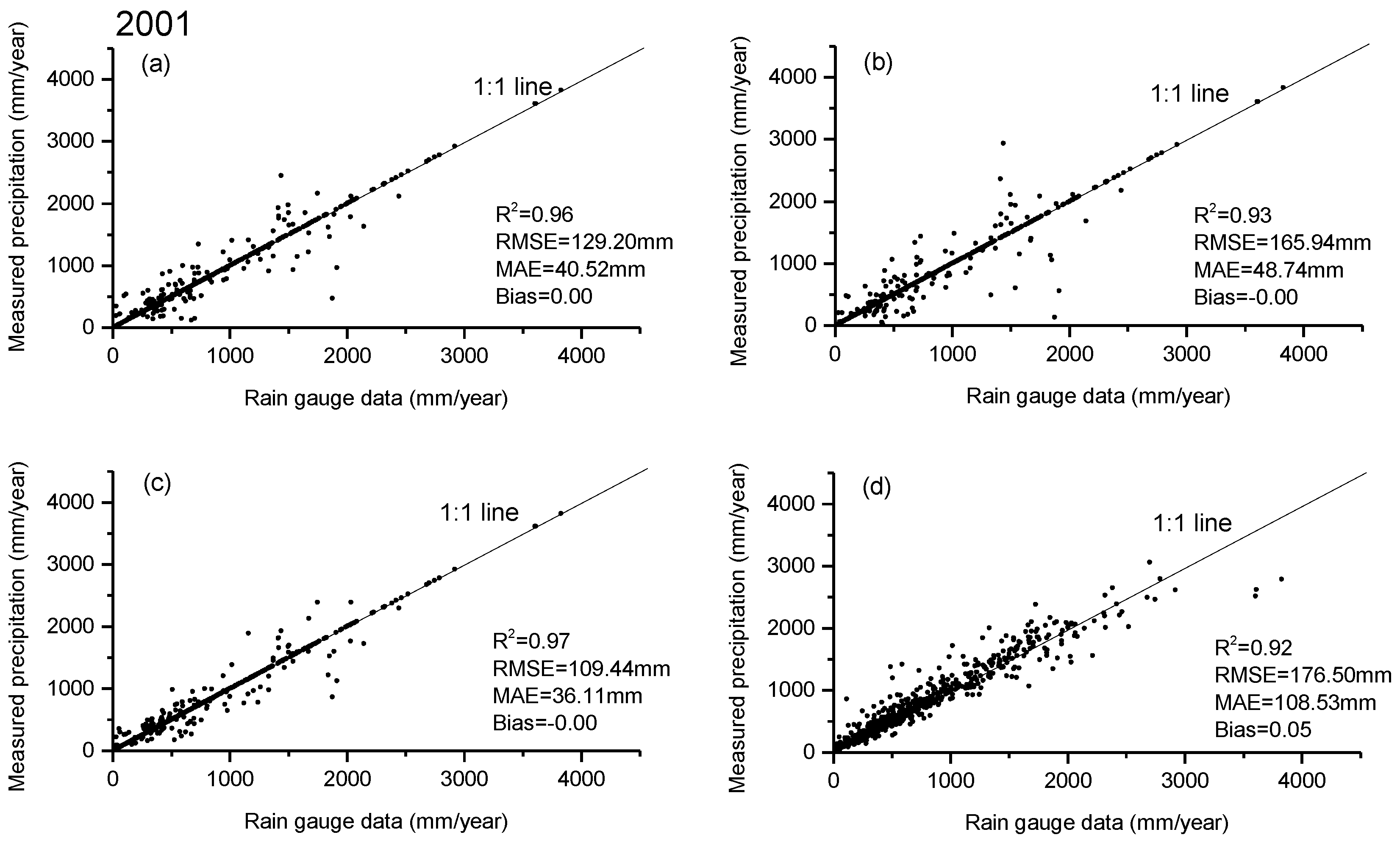
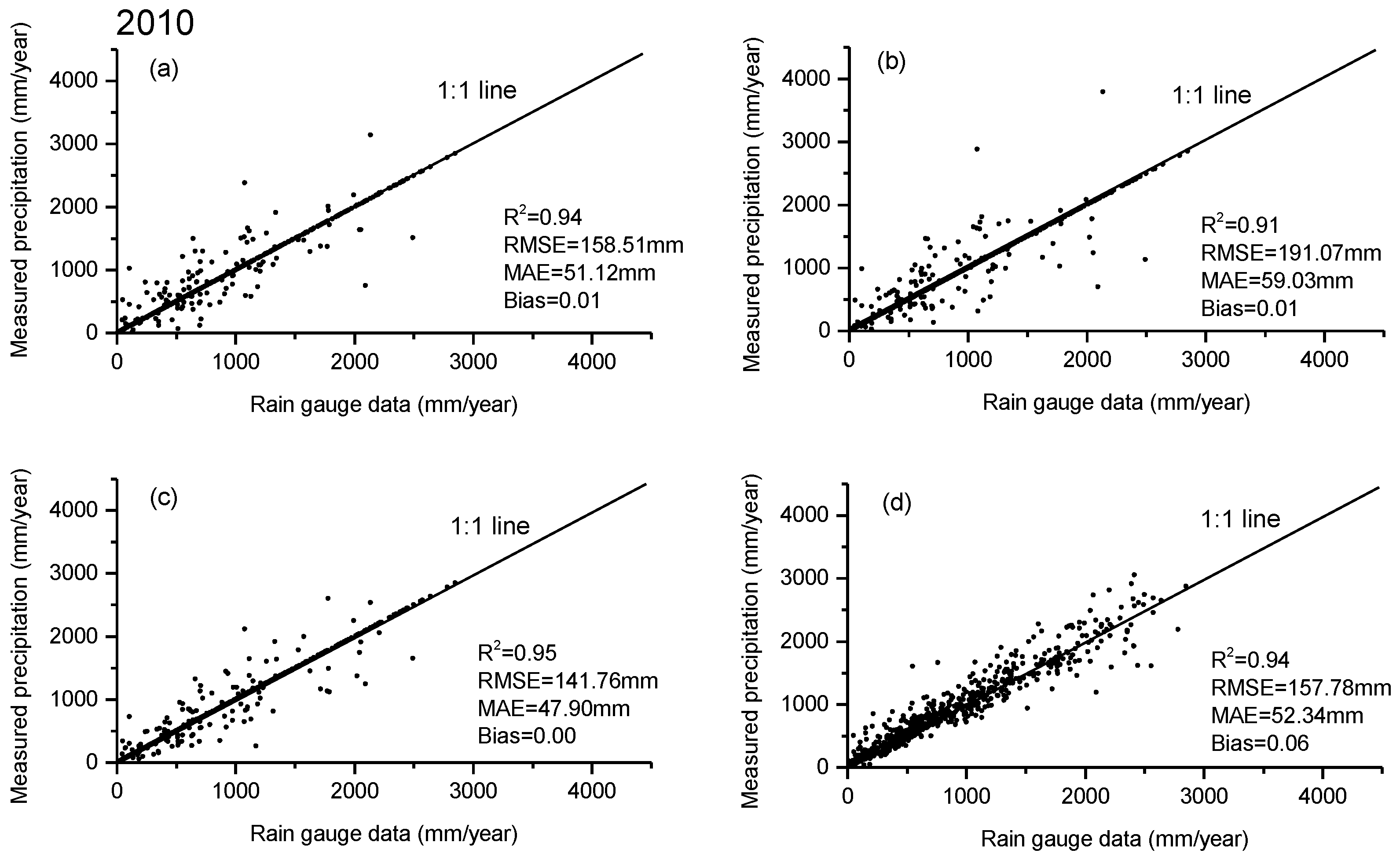
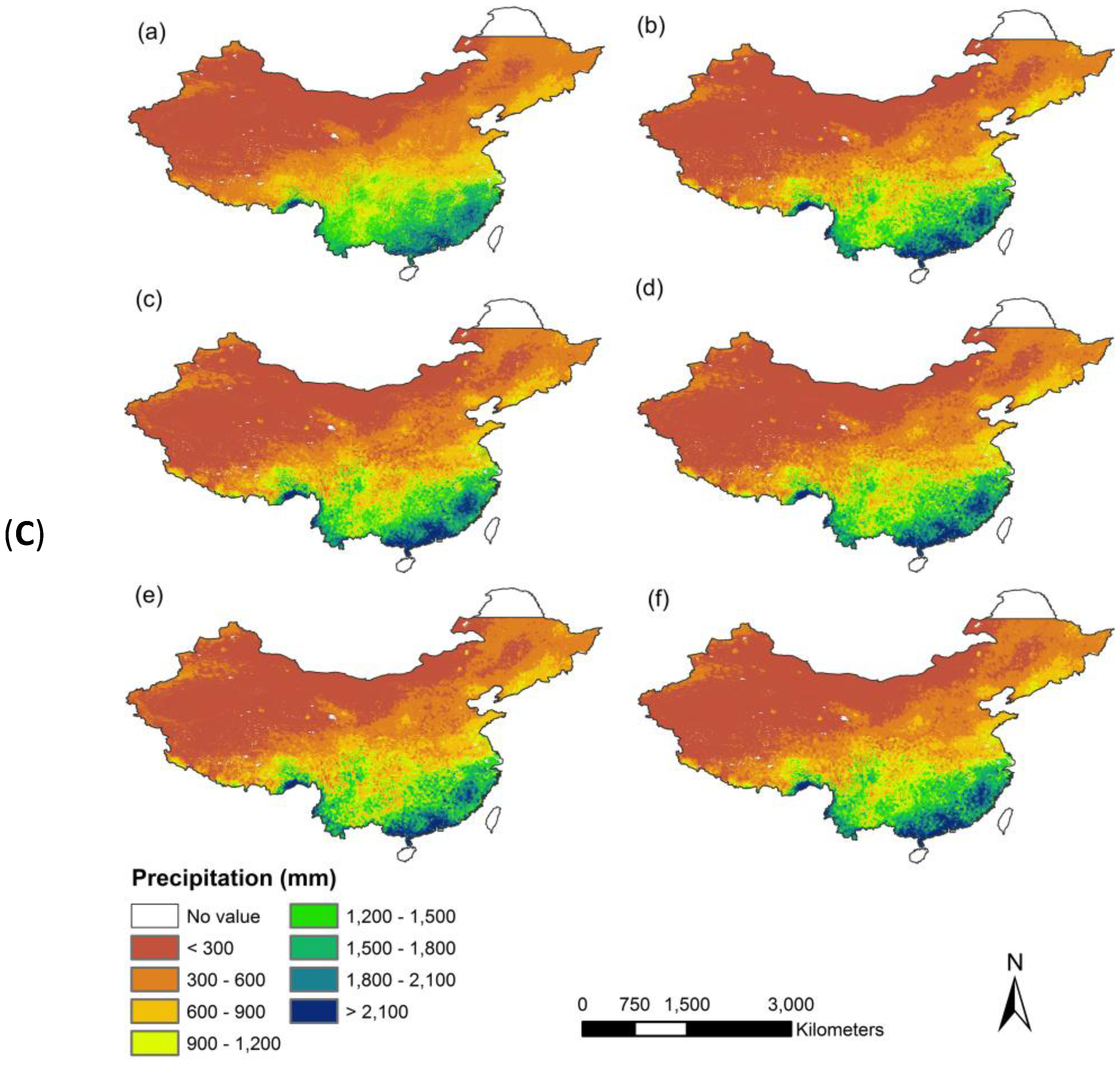
When the downscaled precipitation estimates were compared with the observed station precipitation, the R
2 values are 0.74 in 2001 and 0.75 in 2010 for all the three methods. The efficacy of the three methods was finally validated using the ground observations, collected from 596 meteorological stations of Mainland China for the years of 2001 and 2010 (
Figure 5). As seen from
Figure 5, the RF downscaling approach slightly outperformed among the three regression models in this study in terms of the statistics of R
2, RMSE, MAE, and bias. The results of all years from 2001 to 2010 are shown in
Figure A5.
Figure 5.
Scatter plot of the measured annual precipitation from 596 meteorology stations versus the predicted precipitation derived from (a) the multiple linear; (b) exponential; (c) Random Forest regression model, and (d) original TRMM 3B43 for the years of 2001 and 2010 over Mainland China, respectively.
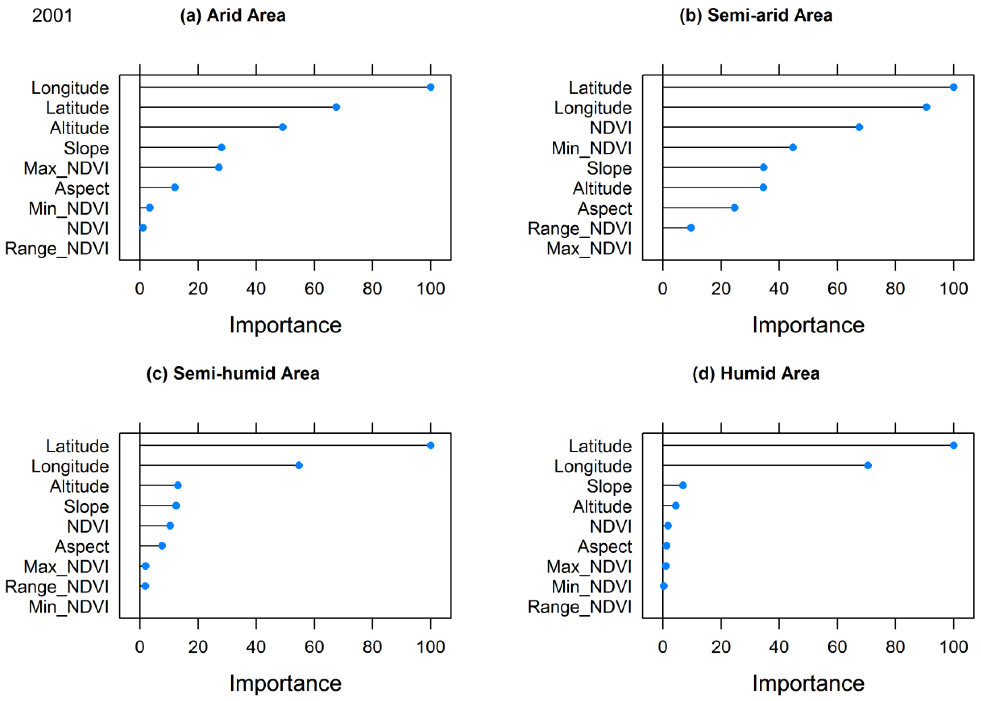
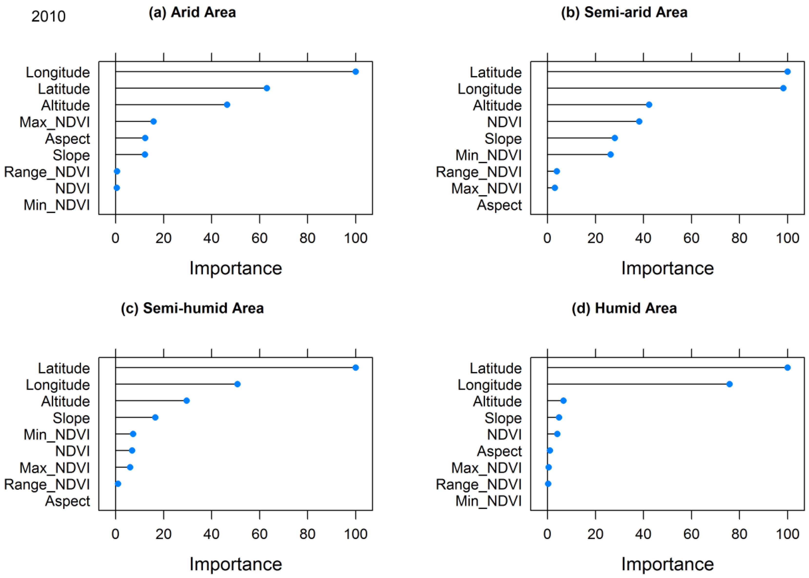
Figure 6.
Importance of geospatial predictors for precipitation downscaling in (a) arid; (b) semi-arid; (c) semi-humid; and (d) humid regions for the years of 2001 and 2010, illustrated by the MDG of attributes as assigned by RF.
Figure 6.
Importance of geospatial predictors for precipitation downscaling in (a) arid; (b) semi-arid; (c) semi-humid; and (d) humid regions for the years of 2001 and 2010, illustrated by the MDG of attributes as assigned by RF.
The importance of input predictors for the RF model is illustrated in
Figure 6. It shows that all nine geospatial predictors play corresponding roles across four climate zones over Mainland China. NDVI-related predictors, such as NDVI, Max_NDVI, and Min_NDVI, represents more importance in arid, semi-arid, and semi-humid areas than in humid areas. Two input predictors, latitude and longitude, make steady contributions to the model simulations unlike the other factors, including altitude, aspect, and slope in four climate zones. The topography-related predictors (altitude, aspect, and slope) were also significant factors for the precipitation downscaling in some areas.
5. Discussion
In this study, three statistical regression approaches were investigated to downscale the TRMM 3B43 precipitation data, and to derive annual precipitation at a 1 km resolution over continental China. We compared the multiple linear, exponential, and RF regression models to better understand how the choice of model type affected the prediction accuracy. We found that (a) the RF regression outperformed, with better R2, RMSE, MAE, and bias values, when compared to the other two statistical regressions; (b) the RF downscaling can well predict annual precipitation of continental China at a 1 km resolution; and (c) NDVI-related variables, latitude and longitude, and elevation are key elements of downscaling method on estimation of annual precipitation from the analyses of variable importance.
We compared the performance of three statistic models in the process of downscaling TRMM 3B43 precipitation and found that RF regression achieved the best results in modeling annual total precipitation in a broad area. It was supported by cross validation of the three models. The RF regression model consistently performed best (
Figure 3) both for the wet year and dry year in term of R
2 (0.97 for two years) and RMSE (94 mm for 2001, and 106 mm for 2010), when compared to the multiple linear regression model (R
2 is 0.77 for 2001 and 0.70 for 2010, RMSE is 258 mm, 314 mm), and exponential regression model (R
2 is 0.68 and 0.66, RMSE is 307 mm and 338 mm). Unlike previous studies [
24,
34,
39], which only used one or two independent variables (NDVI and elevation), the three methods used nine different predictors in this study to establish the regression models. Those newly introduced predictors seem to be necessary for well-fitting regression models in a broad spatial extent since there are relatively weak empirical relationships between precipitation and the saturated NDVI in humid regions. Despite being the most accurate among three statistical models for predicting precipitation and it exhibited considerable improvement from fitting, there are still certain limitations in the RF algorithm. For example, other uncontrolled variables, such as hydrological conditions and human activities, might influence the distribution of NDVI and, hence, cause some errors in the final results; the processing of variables aggregation (e.g., NDVI, elevation, slope, aspect of the terrain) had not taken into account the uncertainties derived from resampling and re-projection of maps and data. In addition, other unknown predictor variables may also contribute to the efficacy of the RF model, thus further investigation would be needed to confirm which and how many factors are related to the total annual precipitation in Mainland China.
From
Figure 3, we can see that all the models seemingly perform better for the areas characterized by low amounts of rainfall. A possible reason may be that NDVI-related predictors are better indicators of precipitation in arid and semi-arid areas. The NDVI values would not increase with the increased rainfall amount in humid areas, which makes a relatively weak empirical relationship between precipitation and saturated NDVI. This could also be seen from the analysis of variable importance (
Figure 6). However, substantial difference of the precipitation maps is found in some regions of Mainland China. The area with extreme precipitation predicted by the RF model is smaller than that predicted by multiple linear, and much smaller than that by the exponential model. The differences among these maps are possibly caused by the added residual terms, or by the performance of the models. Normally, the model’s performance in the validation period is the best indicator as to its ability to predict the future. If a regression model, such as the RF model, can make accurate predictions of precipitation (R
2 > 0.97), the predicted values will be very close to the original TRMM precipitation, and the residual values will be small. The relative weights of the residuals will also become small (
Table 2). Especially in South Mainland China, where a large amount of precipitation (annual precipitation greater than 1200 mm/yr) is received, the relative weight of the residual calculated from the RF model will be significantly smaller than that from the other two models.
The downscaling algorithm with three regression models can well predict annual precipitation of continental China at a 1 km resolution. In terms of RMSE, MAE, and bias, the downscaling approach with the RF model produced the lowest amount of errors compared to the other two statistic regression models when validated using precipitation dataset collected from the meteorological stations for both the wet year and dry year (
Figure 5). The general precipitation patterns are well captured in this estimate by all three regression models. The northwestern part of the Chinese mainland is drier, and the southeastern part and the southern coast are clearly wetter. Those patterns satisfactorily resemble the general spatial distribution patterns of annual precipitation of Mainland Chain [
67,
68].
Through importance analysis, we found that latitude and longitude are very important factors in simulating the annual precipitation over Mainland China. Rainfall in the study area mainly results from the moisture-laden air masses from the Western Pacific and the Indian Ocean. Latitude and longitude may represent the relative distance from the Pacific and Indian Oceans, and, thus, significantly affect precipitation and its spatial distribution. NDVI is generally considered as a powerful predictor for precipitation [
24,
34,
39], but our study resulted in correlations only in arid, semi-arid, and semi-humid zones (annual precipitation less than 800 mm/yr). The higher NDVI does not always represent more precipitation in humid zones because of the saturated NDVI. This leads to a declined importance of NDVI-related predictors in humid areas.
The elevation, another geospatial predictor in downscaling approaches [
24,
34,
39], was used as an indispensable predictor in four climate zones over continental China. Interestingly, the elevation was even more important than the NDVI in humid, semi-arid, and arid areas due to the uplift precipitation effects of mountains and/or the saturated NDVI. Moreover, the importance of the aspect and slope steadily ranked elevation, and these two predictors certainly contributed to the prediction accuracy of precipitation. This is because aspect is linked to the prevalent wind orientation, and, thus, determines the potential relative water excess or deficit; a gradient in the speed of vertical air movements may control the intensity and area of precipitation [
69,
70].
Since the RF technique only pursues the valid regressions between precipitation and geospatial predictors, the geo-physical mechanism is actually not well represented in this approach. Thus, we are still not able to give the explicit mechanistic understanding of precipitation and related predictors. More investigations about the geo-physical mechanism in relation to precipitation would be needed to understand the feedbacks between precipitation and those predictors. This would be also helpful to explore additional geospatial predictors that may improve the RF algorithm. Furthermore, our downscaling framework is currently not applicable to shorter temporal periods (e.g., monthly or seasonal). In the future, monthly or seasonal precipitation can be estimated using, for instance, the fraction method proposed by Duan and Bastiaanssen [
24]. It should be also noted that there is still a scale gap between rain-gauge data and final rainfall product in this study because a rain gauge typically collects rainfall at ground level with a sample area of roughly 50 cm
2 [
71]. It is, therefore, suggested that gap be taken into account in future studies, especially at finer time scales.

 ,
, 


