Next Article in Journal
Modeling Top of Atmosphere Radiance over Heterogeneous Non-Lambertian Rugged Terrain
Previous Article in Journal
Remote Sensing and GIS for Habitat Quality Monitoring: New Approaches and Future Research
 
 
Correction published on 14 January 2016, see Remote Sens. 2016, 8(1), 64.
Article

Estimating Leaf Bulk Density Distribution in a Tree Canopy Using Terrestrial LiDAR and a Straightforward Calibration Procedure

1
Institut National de la Recherche Agronomique, UR 629, Ecologie des Forêts Méditerranéennes, Domaine Saint Paul, Site Agroparc, F-84914 Avignon Cedex 9, France
2
Office National des Forêts, Département RDI-Pôle Nancy 11 Rue de l'île de Corse, F-54000 Nancy, France
*
Author to whom correspondence should be addressed.
Remote Sens. 2015, 7(6), 7995-8018; https://doi.org/10.3390/rs70607995
Submission received: 13 March 2015 / Revised: 9 June 2015 / Accepted: 10 June 2015 / Published: 18 June 2015

Abstract

:
Leaf biomass distribution is a key factor for modeling energy and carbon fluxes in forest canopies and for assessing fire behavior. We propose a new method to estimate 3D leaf bulk density distribution, based on a calibration of indices derived from T-LiDAR. We applied the method to four contrasted plots in a mature Quercus pubescens forest. Leaf bulk densities were measured inside 0.7 m-diameter spheres, referred to as Calibration Volumes. Indices were derived from LiDAR point clouds and calibrated over the Calibration Volume bulk densities. Several indices were proposed and tested to account for noise resulting from mixed pixels and other theoretical considerations. The best index and its calibration parameter were then used to estimate leaf bulk densities at the grid nodes of each plot. These LiDAR-derived bulk density distributions were used to estimate bulk density vertical profiles and loads and above four meters compared well with those assessed by the classical inventory-based approach. Below four meters, the LiDAR-based approach overestimated bulk densities since no distinction was made between wood and leaf returns. The results of our method are promising since they demonstrate the possibility to assess bulk density on small plots at a reasonable operational cost.

Graphical Abstract

1. Introduction

The amount and spatial distribution of foliage in a tree canopy has fundamental functional impacts on ecosystems by affecting energy and carbon fluxes through photosynthesis and transpiration. It governs radiative transfer in canopies, and the turbulent transfer of sensible heat, water and carbon dioxide between the atmosphere and the surface layer. These processes are incorporated in soil-vegetation-atmosphere transfer models (SVATS), in one or three dimensions [1,2,3,4,5,6]. These models have demonstrated that vegetation spatial distribution influences net primary production and water fluxes [3], radiation fluxes and vertical temperature profiles [6] and competition for light [4]. Foliage is also a component of the fine fuel that affects the propagation of forest fires [7] and fire emissions [8]. Its spatial distribution influences heat transfer, wind and fire behavior [9,10,11]. Process-based models for ecosystem functioning or wildfire behavior such as those referred to above either require the determination of leaf area density or leaf bulk density, which are related by specific leaf area (SLA).
The most accurate method for estimating the biomass of a forest canopy is to physically sample it, but this is not feasible on large samples of trees. At forest plot scale, a common method, hereinafter referred to as the inventory-based approach, is to combine a stem inventory and allometric equations for biomass and its vertical cumulative distribution in order to estimate leaf load and bulk density profile [12,13]. However, in order to be robust, allometric equations require significant sampling since leaf biomass does not only vary with stem diameter, but also with crown dimension, competition, stand age, basal area, management practices and even day in the year [13,14,15]. Sensitivity to type of equation for vertical distribution may also be high [13]. Remote sensing techniques have long been used in forest management and research, especially for estimating leaf area index [16]. These techniques include terrestrial LiDAR (Light Detection And Ranging), referred to hereinafter as TLS (Terrestrial LiDAR System), which emerged as a promising tool for leaf biomass or surface area estimation because the distribution of returns can be used to estimate density indices in voxels [17,18], which are volumetric pixels. The indices can be specifically computed for the leaves since the intensity can be used to distinguish leaf from wood returns [19] or finer elements from larger ones [20]. Density index approaches are based on the probability of light transmission, on the contact frequency method [19,21] or on the voxel-based canopy profiling method [22,23]. We will qualify these methods as “direct”, in the sense that they do not require any calibration, even if several assumptions are required to convert the density of LiDAR returns to leaf bulk density. These direct measurements have been used successfully at tree scale but require voxelization of the scanned scene at 0.001 to 0.1 m and multiple scans for a single tree. This is time-consuming in terms of measurements and post-processing, and this may be considered to be a limitation for operational use. Seielstad et al. [20], therefore, used a calibration approach to estimate branch biomass from scans and proposed to use randomized branch sampling to extrapolate to trees. Skowronski et al. [24] used upward sensing profiling paced at a constant rate and calibrated at stand scale using the inventory-based approach. This method provides bulk density profiles at stand scale, but requires calibration from an existing inventory and the destructive sampling of trees. Also, it does not provide a 3D biomass distribution. Calibration of TLS has also been used for fuel and fire effect characterization [25,26,27,28], but never in the past for leaf biomass estimation at plot scale.
Herein, we propose a method to estimate the spatial distribution of leaf bulk density from TLS scans. It is based on the development of indices similar to those used at tree scale in earlier direct estimation studies. Here, the indices are computed in spherical volumes that are larger than the small voxels employed in earlier studies, and a field calibration is used to provide a less time-consuming but still robust estimation of the distribution at plot scale.

2. Material and Methods

2.1. Study Area and Plot Description

The study site is located in Southeast France, in the Saint-Lambert forest (Position: 44°0′16″N, 5°20′59″E; altitude: 780 m). The dominant species is Quercus pubescens with a dominant height of 9 m. A minor presence of other deciduous tree species is noted along with a sparse understory dominated by Juniperus communis. This site was selected from among those of a broader study of Quercus pubescens stands viewed as fuel types. Four contrasted plots were selected for the present study from among the 20 at the site (Table 1). Each plot is circular with a diameter of 12 m (Figure 1) and has flat topography.
Each plot was described by means of a field stem inventory (species, location, stem diameter and height). In the inventory-based approach, leaf bulk density profiles (kg·m−3) and loads (integration of the vertical distribution of the bulk density, in kg·m−2) were derived from the combination of the inventory and regression equations to estimate leaf biomass and vertical cumulative biomass distribution. Regression equations were derived from a sample of 11 harvested trees collected in the study site for the purpose of the present study. The regression equations for the tree leaf mass and for the cumulative leaf weight distribution had, respectively, determination coefficients of 0.91 and 0.95. Additional details are provided in Supplementary A. They include the cost of measurement (over 100 days of labor to get data required for model parameter estimation and four field hours for each stem inventory) and additional statistics (including RMSE and confidence intervals for predictions). Since the inventory-based bulk densities are the most accurate estimations we can get for the study site (without harvesting all plots, which would require tens of person-months), they will be used to evaluate the TLS-based approach developed here.
Table 1. Plot main characteristics.
CharacteristicsPlot 1Plot 2Plot 3Plot 4
Stem number31594265
Max height (m)8.38.410.712
Total basal area (m2·ha−1)18303040
Quercus pubescens %94837185
Note that stem number includes all stems with diameter larger than 2.5 cm. The Quercus pubescens percentage was computed from basal area per species.
Figure 1. Schematic view of Plot 1: The Li (red pentagons) show the position of the TLS. The Ri (gray squares) show the position of the six reference targets used for scan placement. The Bi (black circles) show the positions of the ten polystyrene balls marking out the calibration volume centers.
Remotesensing 07 07995 g001

2.2. Calibration Volumes (CV): Description and Measurement

In each plot, ten polystyrene balls (diameter 0.1 m) were placed at different locations in the canopy (Figure 1 and Figure 2a). Balls were either glued to secondary branches (if low in the canopy) or hung from secondary branches (if high in the canopy) using a pole and a metal hook attached to each ball. The balls were randomly placed in the foliage except that their height was restricted to 8 m for practical reasons.
The balls were used to mark out the center of the Calibration Volumes (CV), which are virtual spherical volumes bounded by the 0.7 m diameter sphere that has the same center as the polystyrene target. The location of each polystyrene ball was measured in the cylindrical coordinate system centered on plot center and north oriented, using a measuring tape for horizontal distance, a pole for vertical distance and a compass for the azimuth. These measurements will only be used as rough estimates of ball locations to identify them within the point cloud.
Once the TLS scans had been performed on a plot, the leaves inside the calibration volume were collected. To facilitate this collection of the material inside the CV, a 0.30 m stick was first used to remove all the material outside the CV (Figure 2b). The collected leaves were then oven-dried at 60 °C for 24 hours and weighed.
For the 40 CV, the cost associated with setting and collection required less than two days of labor for two workers, whereas separating vegetation elements, oven-drying and weighing were on the order of three days of laboratory work for two workers. The total time for processing CV was then 10 days of labor.
Figure 2. Picture of a target used to locate the center of a calibration volume (CV). (a) A polystyrene ball target and (b) removing material outside the CV before leaf collection.
Remotesensing 07 07995 g002

2.3. TLS Instrument and Measurements

A FOCUS 3D 120 S (FARO Technologies Inc., Lake Mary, USA) TLS instrument was used in this study. It is a phase-shift LiDAR that emits modulated laser beam pulses at 905 nm in a 305° (vertical) × 180° (horizontal) view window. Range of use is 0.6 to 120 m (with low ambient light). Beam diameter leaving the instrument is 3 mm, with divergence of 0.19 mrad, such that it was always less than 1 cm inside the plots scanned in this study. Basically, in each scanning direction, the scanner may receive a true returned signal, or echo, when the beam is reflected at sufficient intensity by an opaque surface element in the direction of the scanner. The distance from the scanner to the opaque surface element, and beam direction, define the 3D coordinates of the surface element that defines the data point. The FOCUS 3D has two material filters on its scanner: “Clear Sky” and “Clear Contour”. When scanning into the sky, no actual laser light is returned, but the scanner receives some light from the sky at the same wavelength as the laser (905 nm) at an intensity that can be of the same order of magnitude as real returns. The different phase lengths (used for disambiguating distances in a phase-shift TLS) show a specific pattern when scanning into the sky. This does not occur when scanning real objects (FARO technical support, personal communication). This pattern is used by “Clear Sky” to filter sky returns in the point cloud. Returns can also correspond to a mixing distance of several objects since the laser beam has a finite diameter and may only partially hit objects. This is known as mixed pixel noise [29]. The “Clear Contour” filter uses the different phase lengths of the scanner to identify the specific pattern associated with mixed pixels and filter out these points. The scans in our study were performed with both filters activated, because they remove false points. However, this filtering out of point clouds affects the computation of indices based on the contact frequency method. Corrections to account for these filters are developed in the next section.
Five scans were performed on each plot from the center and from the four corners of the square inscribed in the circular plot (Li with i between 1 and 5 in Figure 1). The scanner was placed 1.3 m above ground level. Resolution angle was 0.036° (43822090 pixels per scan) and measurement speed “x4” (488000 pixels·s−1, which is 24 = 16 fold minimum scanning speed), as recommended for outdoor scanning. Six 140 mm spherical artificial targets (Ri with i between 1 and 6 in Figure 1) were placed in the scene for the five scans of each plot. In general, it is not required to have six targets within the scene, but at least three of them should be seen from each scanning position without occlusion. Additionally, they should be placed so that they do not constitute a narrow angle from the scanner position, otherwise placement is less accurate. Scanning each plot required, on average, one hour of labor for two technicians.

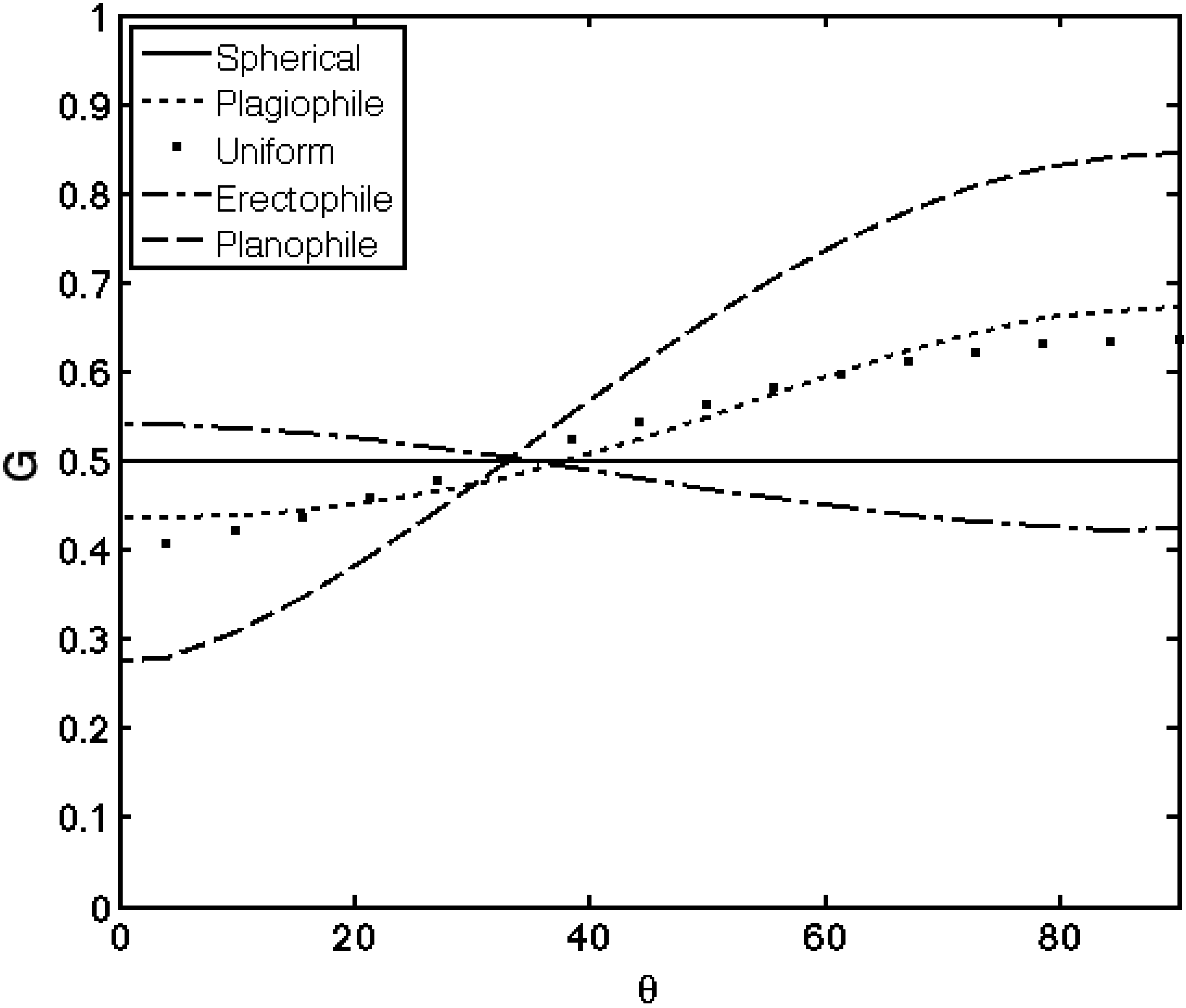
2.4. Definition of Density Indices in Spherical Volumes

In this section, we define three indices that can be derived from scans to estimate vegetation density. These indices were computed for spherical volumes such as the CVs described above, but can theoretically be computed for any volume.
Following [17], we defined an index of element density I in a volume by the number of returns from inside this volume (Ni) divided by the number of beams that effectively went through the volume (estimated by the total number of beams that would go through the volume if no vegetation were present (Nt), minus the number of beams reflected by solid surfaces between the scanner and the volume (Nb)).
I = N i N t N b
To account for leaf orientation, this index can be refined using the G function [30]:
I 1 = N i ( N t N b )   2 G ( θ )
The G function is the surface element projection function that accounts for the surface element orientation [30,19] and is commonly used in models of radiative transfer in plant canopies. θ is the angle between LiDAR beam and zenith. The factor 2 here is for convenience since the G value is 0.5 when the distribution of surface elements is spherical [30,19]). A schematic view of the different returns is shown in Figure 3.
When estimating leaf bulk density ρ as a function of density indices, Ni should be restricted to leaf returns from inside the spherical volume. The authors of [19] showed that for broad leaf trees it was possible to distinguish leaf returns from wood returns using a threshold on the return intensity since leaf reflectance was lower than wood reflectance at the wavelength of their time-flight 1500 nm TLS. Wood must be understood as bark of trunks and branches. The difference between reflectances of wood and leaves is likely due to water content near the surface of these elements: water exhibits an absorption window of radiation near 1500 nm [31]. Working with a similar TLS on coniferous branches, [20] found that a threshold on intensity could also be used to separate the returns of leaves and twigs thinner than 6 mm from thicker wood returns given that the small elements were much smaller than beam size, resulting in geometrically weaker returns. In practice, using the FARO FOCUS 3D, we were unable to determine an intensity threshold to distinguish between the returns from inside the foliage (in the calibration volume) and those from trunks, probably because wood and green leaves may have similar reflectance values at 905 nm [32] and the leaves are far larger than the laser beam. Figure 4 provides intensity distributions for the central scan of Plot 2. Figure 4a shows the intensity distribution of returns from inside CVs, dominated by foliage and small branches located between 3.13 and 6.44 m from the scanner. Figure 4b shows the intensity distribution of returns manually extracted by FARO SCENE 5.1 software in the scan of tree trunks. Trunks were selected at various distances (between 1.12 and 6.87 m) from the scanner such that the range of distances was similar to that in the CVs. Returns from CVs showed a large range of intensity values between 0 and 1, whereas most of the intensities from trunk returns were between 0.75 and 0.85. This showed that leaf (and twig) intensities can either be lower or higher than trunk intensities on a similar distance range. As a consequence, no clear intensity threshold could be identified to separate leaf and wood. Therefore, all returns were considered and index I1 thus corresponds to plant area density (leaf and wood). Here and further, we assumed that leaf area density (and thus leaf bulk density) is proportional to plant area density and that the calibration process took account of the proportionality coefficient. This assumption is realistic inside the crown given that woody elements are mostly thin twigs supporting leaves and their quantity is correlated to the quantity of leaves. However, this assumption is clearly not satisfactory in the lower part of the canopy where plant area density and thus LiDAR returns are mostly dominated by branches and trunks. The consequences of such a limitation are discussed later.
Figure 3. Schematic view of LiDAR return counts around a calibration volume. Nt is the total number of beams emitted in the cone emerging from the scanner and tangent to the calibration volume. It is the sum of the beams intercepted “before” the spherical volume (Nb), the returns from the polystyrene ball (Ne), the returns from vegetation “inside” the spherical volume (Ni), the beams passing through the spherical volume (Ng) and the noise returns in cone filtered by the scanner (Nn). The naming in this figure was adapted from [19].
Remotesensing 07 07995 g003
The formulation used in Equation (2) has other practical limitations arising from scanner properties associated with noise and beam size. The “Clear Contour” filter removes wrong returns associated with mixed pixels, but causes an underestimation of the number of returns before, inside and beyond the spherical volume. The “Clear Sky” filter removes returns associated with sky and thus causes an underestimation of the beams passing through the spherical volume.
Figure 4. Intensity distributions of the TLS point cloud corresponding to: (a) points from inside calibration volumes, dominated by foliage and small branches, and (b) points from trunks at various distances from the scanner. These results show that no threshold on intensity can be used to separate leaf from wood in our scans. NB: Unlike in other studies, intensity was not normalized as a function of distance since the range of distances was similar between the two distributions and sufficiently narrow to assume that distance had no significant effect.
Remotesensing 07 07995 g004
In practice, Equation (2) makes the implicit assumption that all mixed pixels correspond to returns that should have been either in the polystyrene ball (counted as Ne) or beyond the spherical volume (counted as Ng). This holds for returns filtered by “Clear Sky”, but not for those filtered by “Clear Contour”. When a significant number of returns are mixed pixels before or inside a spherical volume (especially in the upper part of the canopy), this causes underestimation of the index. On the other hand, we can make the simple assumption that filtered returns are associated with beams that should have been intercepted before the spherical volume (counted as Nb). This leads to the following formulation:
I 2 = N i ( N i + N e + N g )   2 G ( θ )
For a spherical volume located between the scanner and forest gaps, index I2 leads to an overestimation of biomass since the number of points filtered by “Clear Sky” is neglected, whereas they should have been included in the index denominator. A more rigorous approach is to assume that the returns filtered by “Clear Sky” should be counted as Ng, and that those filtered by “Clear Contour” can be proportionally distributed among Nb, Ni, Ne and Ng. Given that mixed pixels are associated with beams that arrive at the periphery of leaves, and we can assume that their number is proportional to the number of beams that arrives at the central part of these elements. The number of returns from, respectively, inside and before the CV can be estimated by N i ( 1 + f c c ) and N b ( 1 + f c c ) , if f c c is the fraction of points filtered by “Clear Contour” in the cone. This leads to the following formulation:
I 3 = N i ( 1 + f c c ) ( N t N b ( 1 + f c c ) )   2 G ( θ )
Let N n c s and N n c c be the number of returns filtered by “Clear Sky” and “Clear Contour”, respectively. According to the hypothesis of proportional distribution of N n c c among Nb, Ni, Ne and Ng assumptions (as above), we obtain:
N t = N b + N i + N e + N g + N n c c + N n c s   ( N b + N i + N e + N g ) ( 1 + f c c ) + N n c s
Such that N t ( N t N n c c N n c s ) ( 1 + f c c ) + N n c s = f c c ( N t N n ) + N t N n c c and the filtering factor is:
f c c N n c c / ( N t N n )
It can be shown that if N n c s = 0 , indices I2 and I3 are equal.

2.5. Processing TLS Data

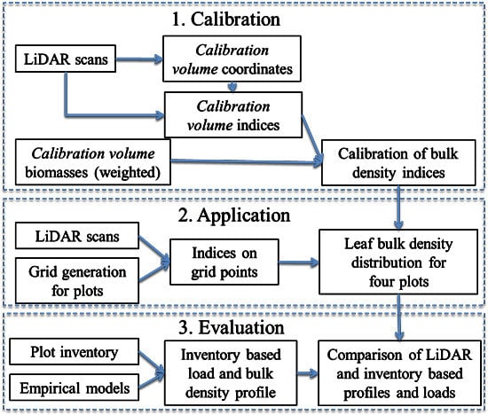
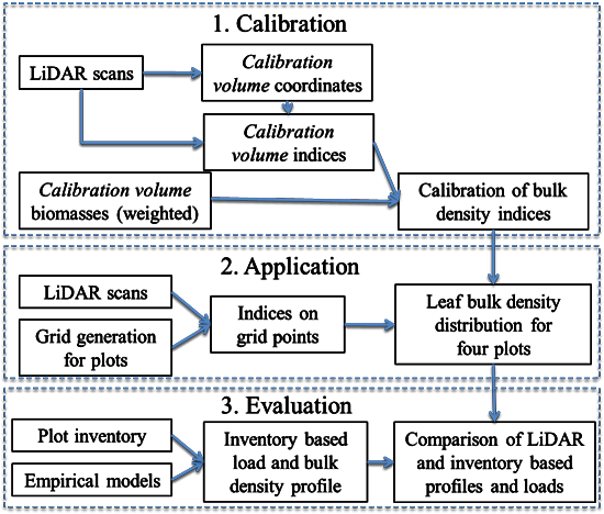
2.5.1. General Framework

For each plot, the TLS returns were first used to compute—by FARO SCENE 5.1 software (Section 2.5.2)—the coordinates of the CV centers in the Cartesian system resulting from the scan placement. Then, for each scan, the biomass indices were computed for each CV. These computations first required the retrieval of information on filtered points in order to compute Nt and fcc (see Supplementary B). The indices were then compared with bulk density data derived from field measurements in each CV (Section 2.2), to calibrate the parameters of the bulk density models (Section 2.5.3). Finally, these models were applied to the grid nodes in each plot to estimate leaf bulk density distributions (Section 2.5.4).

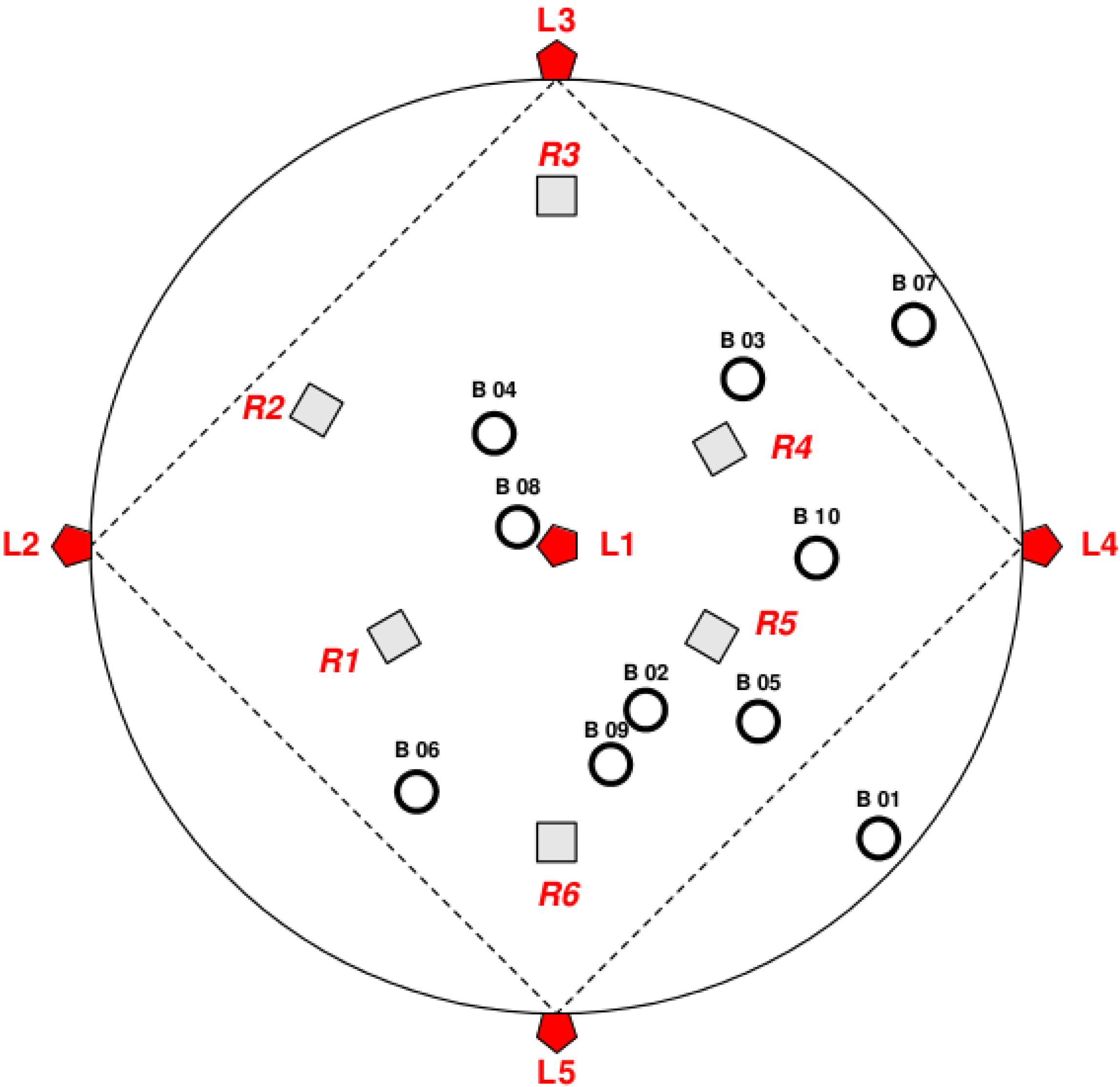
2.5.2. Computation of Calibration Volume Locations

For a given plot, the cylindrical coordinates of each polystyrene ball (measured in the field, Section 2.2) were converted into spherical coordinates in each scan system. When a given scan was opened using the FARO SCENE planar viewer, we sought out each polystyrene ball at the approximate location defined by its spherical coordinates. When the ball was visible, the software’s “sphere ray” tool was used to fit a virtual sphere on the ball. When the fit was satisfactory, we obtained the coordinates of the ball center (i.e. the CV center) in the Cartesian system common to the five scans. When the fitting was unsatisfactory (according to the criteria of the “sphere ray” tool for which accuracy is of the order of 1 mm), we clicked on the ball’s center to get the spherical coordinates (distance, azimuth and zenith angles) of this point, which is at the intersection between the sphere and the straight line passing through the scanner and the ball center. The spherical coordinates of the CV center (ball center) were estimated from the coordinates of the measured point on ball (adding 5 cm to the distance value). We then converted its coordinates into the Cartesian system (manual method). This method enabled us to obtain between 0 and 5 sets of Cartesian coordinates for a CV depending on the number of scans in which the ball was visible. To obtain a single, unique position for each CV, we averaged the different positions obtained by the “sphere ray” method, when at least one position was available. When the “sphere ray” method did not function on any scan, we averaged the positions obtained by the manual method, provided that at least two positions were available and the difference between coordinates was less than 10 cm. The computation of calibration volume locations took approximately one day.

2.5.3. Model Calibration over Calibration Volumes

The coordinates of each CV and the five scans with extended information about filtered returns were used to compute I1, I2 and I3 by a MATLAB script (MATLAB Release 2013b, The MathWorks, Inc., Natick, MA, USA). Processing scans took approximately one day. The scan providing the best view on the CV was selected based on two distinct criteria: largest number of returns in the CV and largest number of beams entering the CV, referred to as (Ni)max and (NtNb)max, respectively. The authors of [19] initially used the second criterion.
Regressions to the origin of leaf bulk density data in relation to the indices were fitted for all three indices and both scan selection criteria. We also tested several hypotheses regarding leaf orientation distribution (Figure 5).
Figure 5. Several projection functions (G) of the zenith angle (0 is horizontal; 90° is vertical) used to compute indices I3.
Remotesensing 07 07995 g005
Let ρ ˜ ( I ) be the LiDAR estimated bulk density for index I and nc be the number of calibration volumes. Following [33], the 95% confidence interval of ρ ˜ ( I ) predicted by the regression equation (calibration) at index value I is:
ρ ˜ ( I ) ± t ( n c 1 ,   1 0.95 / 2 ) σ ˜ c ( I )
with the standard error of the prediction σ ˜ c ( I ) , given by:
σ ˜ c ( I ) = σ c 1 + 1 n c + ( I I m ) 2 j = 1 ,   n c ( I j I m ) 2
where I j are the different values of index I in the nc CV, I m the mean value of I j , and σ c the root mean square error of the regression.

2.5.4. Model Application to Bulk Density Estimation

We generated a 3D grid for each plot. Grids were uniform with a 0.7 m step. Models for estimating the bulk densities of leaves were applied to each grid point to estimate local leaf and twig bulk density in spherical volumes of diameter 0.7 m, centered on grid nodes. These discrete 3D bulk density distributions were then averaged horizontally over plot area (6 m radius disk) to build bulk density profiles at plot scale as a function of height in plot z. At a given height, the number of grid points N1 is 233. Let ρ ¯ ( z ) be the mean actual bulk density in the slice ϑ ( z ) of height dz = 0.7 m. ρ ¯ ( z ) = 1 / V ( x , y , z ) ϑ ( z ) ρ ( x , y , z ) d x d y d z . ϑ ( z ) has a volume of V = 0.7 π 6 2 .
Let ρ ˜ ( i ) be the LiDAR estimated bulk density on a given volume v = 4 / 3 π 0.35 3 inside ϑ ( z ) . The mean LiDAR-estimated bulk density for the whole slice ρ ˜ ¯ ( z ) can be computed by partitioning the volume ϑ ( z ) with V/v volumes (assuming for simplicity that V/v is an integer). Let ϑ 1 ( z ) be the union of the N1 spherical volumes with centers on grid points in the slice ϑ ( z ) . Let ρ ˜ ¯ 1 ( z ) be the mean LiDAR-estimated bulk densities averaged for the N1 spherical volumes of ϑ 1 ( z ) , which are centered on grid points of the slice. The actual mean bulk density at z height can then be written:
ρ ¯ ( z ) = ρ ˜ ¯ 1 ( z ) + [ ρ ρ ˜ ¯ ( z ) ] + [ ρ ˜ ¯ ( z ) ρ ˜ ¯ 1 ( z ) ]
Equation (9) illustrates that when estimating the mean bulk density ρ ¯ ( z ) with ρ ˜ ¯ 1 ( z ) , the resulting error is the sum of the error of LiDAR estimates in slice (mean model error over V/v values) and of the error due to grid discretization on N1 values, instead of the V/v values.
The mean error of the model in slice ϑ ( z ) can be estimated from the standard errors of the prediction σ ˜ c ( I ) of the V/v values:
j = 1 , V / v σ ˜ c ( I j ) 2 ( V / v ) 2 = j = 1 , V / v σ ˜ ( I j ) 2 V / v 1 V / v
We can use the N1 actual measurements of Ij computed on grid points and Equation (8) to estimate the quadratic mean of model error in points of slice ϑ ( z ) . Assuming that the model has no bias and that each measurement is independent, the 95% confidence interval of the mean error of the model in slice ϑ ( z ) is given by:
± j = 1 , N 1 σ ˜ c ( I j ) 2 N 1 1.96 V / v
A rough estimate of the error associated to grid discretization can be computed assuming that ρ ˜ ¯ is the mean of a sample of random values of ρ ˜ taken in ϑ ( z ) . Estimating the standard deviation σ ( ρ ˜ ) with the N1 values of ρ ˜ computed on the grid points, the 95% confidence interval of the error due to grid discretization is given by:
± σ ( ρ ˜ ) 1.96 N 1
This confidence interval is probably overestimated in Equation (12) since ρ ¯ is the mean of a finite number of ρ ˜ values that are spatially correlated.
Bulk density profiles were summed over the vertical direction and multiplied by dz = 0.7 m to estimate loads at plot scale. A similar work as above can be done to estimate confidence intervals for loads.

3. Results

3.1. CV Data

In all, 37 of the 40 polystyrene balls used for CV center location were detected on at least one of the 20 scans using the cylindrical coordinates measured in the field. The others were not detected on any scan due to occlusion. Two of the 37 CVs detected were not used for the calibration process given that either the manual method provided only one center position or the different estimated positions were inconsistent. The disagreement between the positions measured by TLS and those measured in the field (which are far less accurate than by the LiDAR method) was on average 0.15 m horizontally and 0.07 m vertically, with errors consistently less than 0.23 m. These errors are much smaller than the minimum distance between CV, illustrating that the leaf masses in CV were correctly associated with the LiDAR-estimated CV locations. The CVs showed a wide range of leaf and twig bulk densities (Table 2).
Table 2. Main characteristics of the 35 Calibration volumes.
CV CharacteristicsMeanMinMaxStandard Deviation
Leaf bulk density (kg·m−3)0.1670.03880.3130.0595
Center height (m)4.231.697.831.37

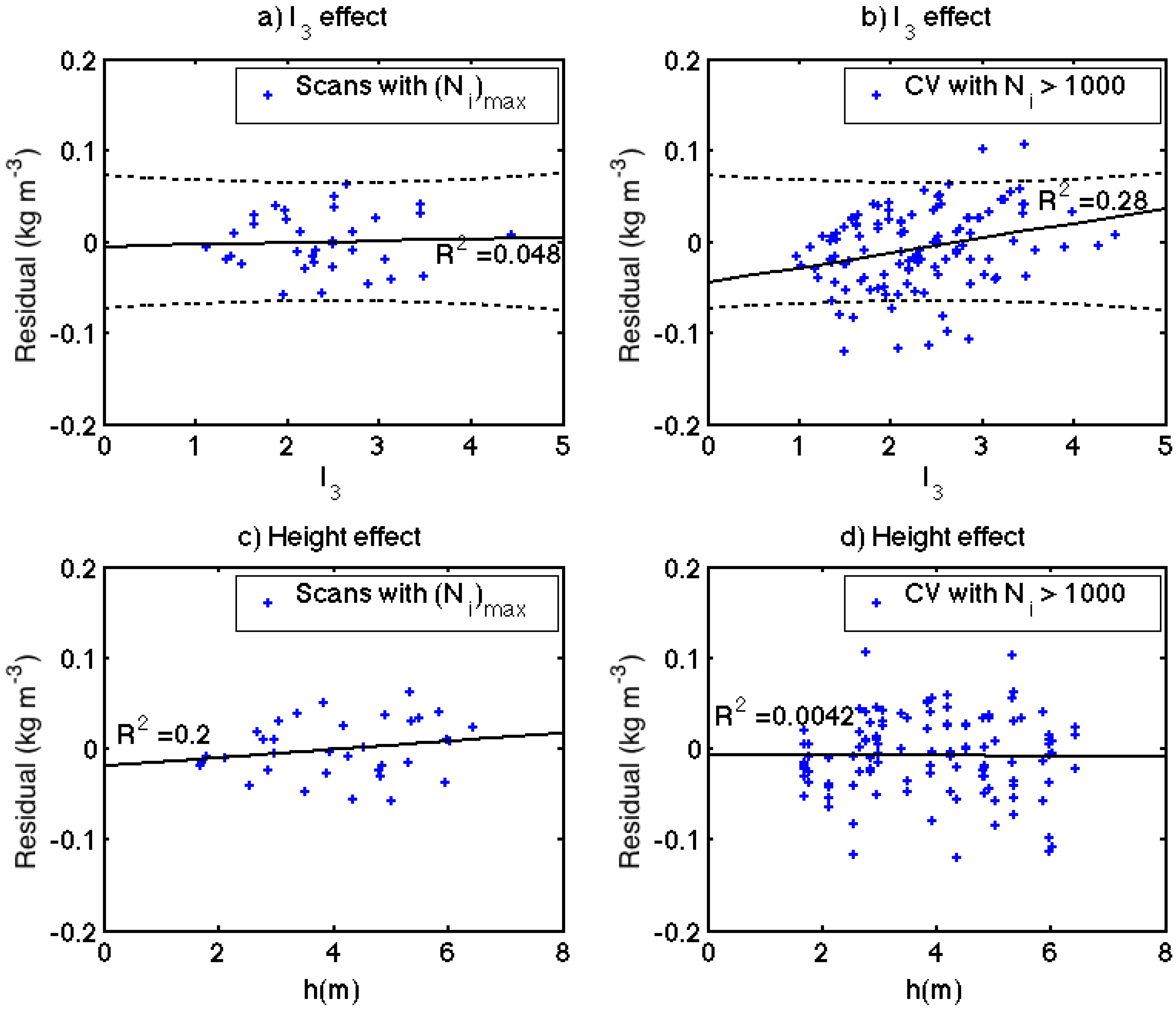
3.2. Model Calibration

Figure 6 shows the calibration of leaf bulk density over the 35 selected CVs for the three indices I1, I2 and I3. Figure 6a,c,e used the largest number of returns in the CV for scan selection ((Ni)max), whereas Figure 6b,d,f used the largest number of beams entering in the CV ((NtNb)max). The determination coefficients exceeded 0.37 for all indices and both criteria, but it was only satisfactory with index I3 and the (Ni)max criterion (R2 = 0.73). The largest number of returns in the CV ((Ni)max) was a slightly more accurate criterion than the largest number of beams entering the CV used by [19]. In addition, the calibration coefficients were less variable for index I3 than for I1 or I2 (Table 3). The model confidence intervals at 95% (dotted lines) were estimated using Equation (8). These intervals overestimate the error for the lowest bulk density, since the model will never provide negative estimates of bulk density.
Figure 6. Calibration of indices I1, and I2, I3 against leaf bulk densities in 35 CVs for the two scan selections, (Ni)max and (Nt − Nb)max: (a) and (b) Index I1; (c) and (d) Index I2; and (e) and (f) Index I3. Dashed lines are 95% confidence interval.
Remotesensing 07 07995 g006
Table 3. Bulk density model characteristics.
Index IElement DistributionCriteriaCalibration ParameterStandard ErrorR2R2 (on CV with Ni > 1000)
I1Spherical(Ni)max0.09580.00350.60−0.19
I1Spherical(NtNb)max0.09730.00430.42−0.16
I2Spherical(Ni)max0.06760.00260.530.34
I2Spherical(NtNb)max0.07280.00310.370.36
I3Spherical(Ni)max0.07230.00210.730.45
I3Spherical(NtNb)max0.07400.00270.600.45
I3Plagiophile(Ni)max0.07670.00220.740.32
I3Uniform(Ni)max0.07760.00220.740.29
I3Erectophile(Ni)max0.07820.00250.600.36
I3Planophile(Ni)max0.07640.00390.22−0.78
The fitted coefficients, standard errors and determination coefficients are specified in Table 3. The scan selections discussed above restricted the calibration process to scans that had the “best view” of the CVs (according to selection criteria). In order to evaluate index performance with more occlusion and/or at greater distances from the scanner, we also used a weaker selection criterion, i.e. the number of returns in the CV had to exceed 1000 (criterion Ni > 1000). In this dataset, a given CV bulk density was potentially associated with indices derived from several scans. The determination coefficients of each model on the scans corresponding to Ni >1000 are shown in the last column in Table 3. As expected, I1 performed poorly because the assumption that all filtered returns could be counted as “Ng” was incorrect when occlusion was significant. I3 performed better (R2 = 0.45).
Figure 7 shows the residuals of the model derived from I3 with the (Ni)max scan selection criterion in order to investigate potential bias of this bulk density model. Residuals were computed as a function of I3 to evaluate potential bias due to vegetation density and as a function of height in the canopy to evaluate potential spatial bias. They were computed on the (Ni)max data (Figure 7a,b) and on the Ni > 1000 data (Figure 7c,d). No significant bias was identified, except a minor one on the Ni > 1000 data (Figure 7b). In this later case, the model could underestimate the highest leaf bulk densities in case of high occlusion or of a long distance between the spherical volume and the scanner. Again, the plots of Figure 7 demonstrate that estimated confidence intervals are overestimated for low density of returns. These results illustrate that assumptions made for index I3 lead to sound results and increased confidence regarding index I3. This index was preferentially used for in the model application that follows.
We also assumed that foliage orientation was not spherical (i.e., that the G function was not constant, see Figure 5) and tested it with the (Ni)max scan selection criteria over (Ni)max and Ni > 1000 data (Table 3). Index I3 performed far better for spherical, plagiophile and uniform distributions than for erectophile or planophile distributions. We retained the working hypothesis that the distribution was spherical since its performance was better in cases of occlusion given that the model’s determination coefficient was much higher than for models with Ni > 1000.
We also assumed that foliage orientation was not spherical (i.e., that the G function was not constant, see Figure 5) and tested it with the (Ni)max scan selection criteria over (Ni)max and Ni > 1000 data (Table 3). Index I3 performed far better for spherical, plagiophile and uniform distributions than for erectophile or planophile distributions. We retained the working hypothesis that the distribution was spherical since its performance was better in cases of occlusion given that the model's determination coefficient was much higher than for models with Ni > 1000.
Figure 7. Analysis of residuals of the model based on I3 and the (Ni)max: (a) function of I3 on the (Ni)max data set; (b) function of I3 on the Ni > 1000 data set; (c) function of calibration volume heights on the (Ni)max data set; and (d) function of calibration volume heights on the Ni > 1000 data set.
Remotesensing 07 07995 g007

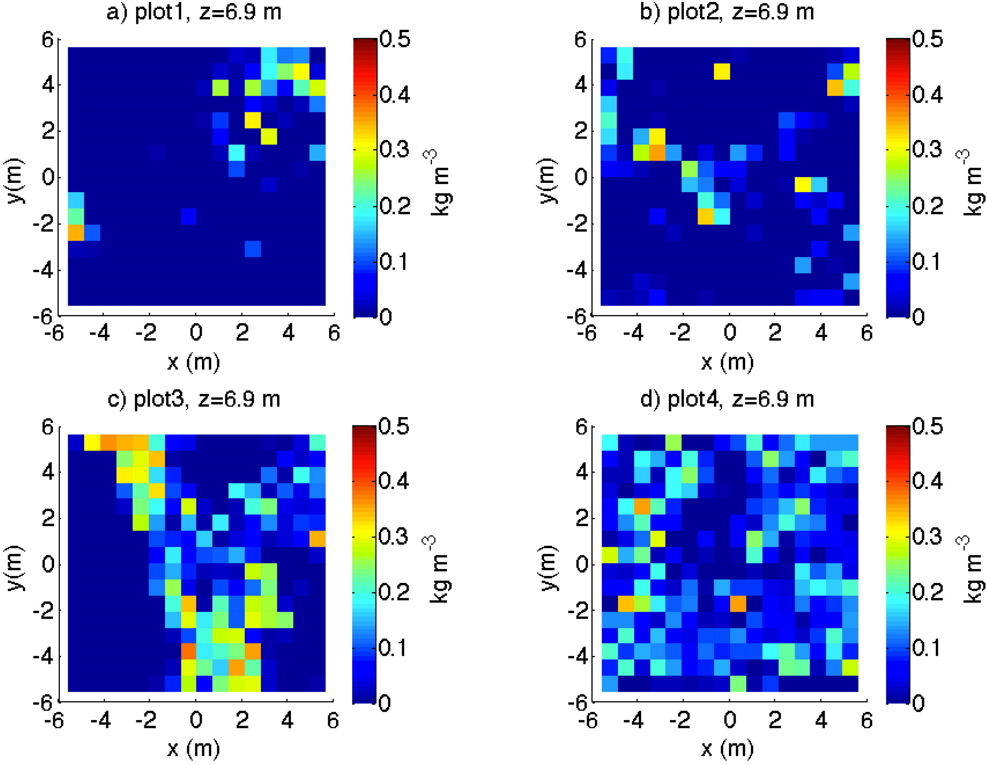
3.3. Model Application and Evaluation

The models derived from indices I1, I2, and I3 were used to build leaf bulk density distributions for each plot. Figure 8 shows the TLS- and inventory-derived leaf bulk density profiles. Variations in height and maximum bulk densities between plots, and the general shape of profiles, were in good agreement except in the lower part of the canopy (mostly below 4 m) where TLS-derived values clearly overestimated inventory-derived values. This overestimation was not caused by shrubs or trees with stems less than 25 mm in diameter (not accounted for in the inventory-based method), since they were less than 2 m in height, but by the interpretation of woody element returns as leaves, as mentioned in the method section. This is supported by Figure S2 (Supplementary A) which shows that more than 90% of the mass of woody elements of diameter >25 mm were below 4–5 m in height in Plots 1, 2 and 3. In Plot 4, the 90% threshold was reached at 6 m, suggesting that the LiDAR prediction may be accurate only above 6 m.
Figure 8. Leaf bulk density profiles estimated from TLS- and inventory-based methods: (a) Plot 1; (b) Plot 2; (c) Plot 3 and (d) Plot 4.
Remotesensing 07 07995 g008
Because it neglected the returns that were removed by “Clear Contour” filtering, index I1 underestimated bulk densities in the upper part of the canopy, and maximum tree height. Index I2 slightly overestimated leaf bulk densities, which could be assigned to the returns filtered by “Clear Sky” (see Section 2.4). Index I3 took account of both filters and provided results that were mostly in agreement with inventory profiles above 4 m.
Using Equations (11) and (12), confidence intervals were computed for index I3 and are plotted on Figure 9. Most of the inventory-based points fell in the confidence intervals of the LiDAR-based method. For reasons explained above, some of the inventory-based points were out of confidence intervals of LiDAR-based method in the lower part of canopies, mostly below 4 m. It was also the case at several heights in Plot 2 and below the bulk density peak in Plot 4. In Plot 2, the LiDAR predicted a slightly higher biomass than the inventory approach, with larger estimations of bulk density in the upper part of the canopies and lower below 5.5 m.
Figure 10 shows the comparison between leaf load predictions by TLS (using index I3) and the inventory restricted to the upper part of the canopy (above 4 m), in order to eliminate bias due to the presence of trunks and branches in the lower part of the canopy. In this restricted zone of the canopy, the convergence between TLS and inventory was very marked and the two methods very similarly reproduced the load gradient between the four plots. Although the profiles were different between the two methods in Plot 2, no visible difference can be seen on their loads, suggesting that differences were only due to spatialization of biomass. The load of Plot 4 was estimated higher with the inventory method than with the LiDAR.
Figure 9. Leaf bulk density profiles estimated from I3 with their confidence intervals (dashed lines) and inventory-based methods: (a) Plot 1; (b) Plot 2; (c) Plot 3 and (d) Plot 4.
Remotesensing 07 07995 g009
Figure 10. TLS-based (using I3) against inventory-based leaf loads above 4 m. The horizontal and vertical bars represent the confidence interval at 95% for both inventory and TLS approaches.
Remotesensing 07 07995 g010
Examples of leaf density horizontal slices derived from TLS are plotted on Figure 11. It shows that the bulk density at a given height (here 6.9 m) varied along the x- and y-axis, depending on tree clumps and canopy structure and is very different from one plot to another.
Figure 11. Horizontal leaf bulk density derived from TLS in Plots 1 to 4 at z = 6.9 m: (a) Plot 1; (b) Plot 2; (c) Plot 3 and (d) Plot 4. The point (0,0) corresponds to plot center.
Remotesensing 07 07995 g011

4. Discussion

4.1. Method Performance for LiDAR-Derived Bulk Densities

In the study presented herein, the calibration process employed yielded encouraging results. The determination coefficient of 0.73 for index I3 (Figure 5c,f,i) shows that the assumptions made for the processing of noise and occlusion were reasonable. Similar conclusions can be drawn about the assumptions of spherical foliage orientation and the proportionality between leaf bulk density and index even without leaf and wood separation. The clearly linear (Figure 6e) relationship between the index and the leaf bulk density over a range of bulk densities (0.039–0.31 kg·m−3) shows that the spherical volume used for the calibration was appropriate in size. Were this volume to be too large, the occlusion inside the calibration volume would induce saturation of the index with leaf biomass.
The specific processing of noise described in this study was necessary when using our phase-shift TLS. This type of TLS has become very popular in forestry because of its low cost and high scanning speed. It is apparently more prone to the mixed-pixel effect [29] than is time of flight TLS. Mixed pixels can often be filtered out by manufacturer tools, such as the “Clear contour” filter, used here. In our study, we used these filters to avoid false returns and also made post-processing corrections. This option provided satisfactory results in terms of calibration and estimated bulk density distribution compared with the inventory-based method. We believe that this approach is more satisfactory than using unfiltered data that is associated with a large number of false returns between different elements of vegetation.
The hypothesis of spherical distribution for foliage orientation was satisfactory since none of the classical orientation functions tested provided significantly better results. This finding is in agreement with those of [20] who obtained similar correlations between their indices and fine fuel biomasses of coniferous branches regardless of orientation.
The hypothesis of proportionality between leaf bulk density and TLS index provided reasonable results in the upper part of the canopy, but did not hold in the lower part where trunks and large branches were dominant. This is a weakness of the present study, but may be attributed to the specific TLS wavelength employed (905 nm) rather than to the method itself. The determination coefficient of the calibration would have probably been better had the leaf returns been separated from the wood returns.

4.2. Accuracy and Cost Comparison of Inventory- and LiDAR-Based Method

Inventory-based profiles and loads have their own limits that could lead to an overestimation of biomass in high basal area plots, such as Plot 4, and to an underestimation of biomass in the lower part of canopies (see Supplementary A). It was not possible to compute confidence intervals for the inventory-based profiles, because the derivative of the fitted cumulative equation (Supplementary Material A, Figure S1b) was used to compute the profiles. However, the confidence intervals computed for loads were wider for inventory than for TLS method, which indicates that TLS-derived data using I3 have the potential to be at least as accurate as inventory-based data in parts where trunks and large branches are negligible.
The time associated with model calibration for the inventory and LiDAR-based were, respectively, of 100 and 12 days of labor (including field work, laboratory work and data processing). The working time per plot was of the same order of magnitude for both methods (when including post-processing of LiDAR data). When based on DBH only, allometric equations lack of robustness for being applied to sites other than the ones where measurements were made. More complete allometric equations, that include crown dimension, competition, stand age, basal area, management practices, etc. are robust between sites [13,14,15], but requires a much larger data collection that in the present study. For the reasons stated below, the LiDAR calibration for a given species or group of species could be much more robust. As a consequence, the model development for the LiDAR method is at least eight times faster than for the inventory-based method. The measurement time of a given plot is similar, but the data provided by the LiDAR method are tree-dimensional, whereas the inventory approach only provided vertical distribution.

4.3. Benefits and Drawbacks of Calibration vs. Direct Estimation by LiDAR

Leaf area density at plant scale has in the past been estimated directly by several authors [19,21,22,23]. This direct approach required a determination of leaf angle distribution, a correction for laser beam size, and very small voxels (between 1 mm and about 10 fold leaf size) to avoid inaccuracies caused by local heterogeneity (Jensen inequality, see [9,34,35]). At the same time, the number of beams entering a given voxel must be high. This requires a number of high resolution scans per tree and reconstruction of occluded areas. One of the main benefits of our calibration approach is that the spherical volume has a length scale 10-fold the size of the voxel in the direct approach [19,21,22,23]. Far fewer scans are therefore required to obtain a satisfactory view of the spherical volume. Computational costs are also greatly reduced since the number of volumes increases with the third power of the inverse of the grid step and index computation is faster on a sphere than on square boxes. Our current calibration approach is suitable for a small plot, but could also soon be operational on larger plots.
The cost of the calibration procedure is a limitation, especially if the calibration coefficients show poor stability. However, we expect these coefficients to be relatively stable as they depend only on the distribution of foliage element at the spherical volume scale, which should be relatively stable between plots. For a given species (or group of species with similar morphologies), we can expect variations to be limited and potentially predictable from element characteristics, such as SLA.

4.4. Future Work

Probably the first requirement for future method development would be to apply similar methodology but with a scanner able to distinguish leaf from wood returns [19,21]. The second step would be to enhance confidence in the indices and calibration coefficients by applying the method to various species and plant morphologies at calibration volume scale and thereby determining calibration coefficient variations. This would be useful for multispecific forests. Another aspect worthy of investigation is the application of a similar calibration methodology to thin twigs in a context of fuel measurements [20]. This was not possible here because of the LiDAR wavelength selected. The last step would be to optimize the number of scans and the spatial arrangement of scanning positions to increase sampling speed in slightly larger plots (20 m or more). The process should culminate in the development of an efficient, non-destructive, operational method that can be used to estimate 3D leaf and twig bulk density distributions in forest plots at a reasonable cost.

4.5. Applications

The development of efficient methodologies to estimate biomass distribution accurately is of great importance in order to capture the variability between stands of similar species composition arising from differences in climate, slope, soil fertility, forest management, stand age, and history of land use. All the aforementioned factors may impact the amount and distribution of foliage in the canopy. A non-destructive methodology is also well suited to monitoring the impact of disturbance and climate change over time.
In addition, compared to the inventory-based approach, the TLS-based approach provides a full characterization of the 3D spatial distribution of foliage in addition to the vertical profiles of leaf area or biomass that are usually produced. Fire behavior in stands with similar load and bulk density profiles is expected to differ if their internal spatial arrangements are different [10,11]. The probability of transition from surface to crown fire in conifer forests depends on some bulk density thresholds and decreases with crown base height [36,37]. However, these common metrics do not account for horizontal continuity between fuel clumps, which is also known as a factor for transition from surface to crown fire. 3D distributions of leaf bulk density estimated with TLS can be used to compute new metrics that accounts for fuel heterogeneity (e.g. in Supplementary C).
Estimations of the 3D distribution of leaf quantities are also very promising as input data for process-based models of stand functioning or fire behavior. Airborne LiDAR data have already been used to assess vegetation structure in SVAT models [5] or fire behavior models [38], but tree height and crown base height are the best output data of these methods. To the best of our knowledge, TLS-derived bulk density distributions have never been used, but were cited as promising [4]. The method presented herein is a good candidate to provide input data for these models given that its averaging scale (0.7 m) is of the same order of magnitude as the voxel size of 3D physically-based models, generally about 1 m [6,10]. Highly variable spatial distributions of leaf bulk density (Figure 11) suggest that some impact of vegetation structure can be expected on model predictions. In addition, our method could be used to provide accurate input data for physics-based fire models in validation exercises such as those done on ICFME [39].
Efficient, operational methodology to estimate leaf distribution characteristics also has a great deal of potential for a combined application with data derived from airborne and space-borne remote sensing. These techniques provide very promising extended maps, but often require ground measurements for calibrations. The method presented herein could be used to measure leaf distribution characteristics on small plots that could then be combined with airborne and space-borne remote sensing techniques. For example, satellite images are used to remotely identify fuel types, but there is no efficient method to evaluate fuel loads associated to the each fuel types.

5. Conclusion

The present study describes a new method to estimate the three-dimensional leaf bulk density of tree canopy in small forest plots, based on a simple calibration of indices derived from T-LiDAR point clouds. Several indices were calibrated over spherical volumes from actual bulk density measurements. One of them accounted for noise and occlusion and used the highest density of returns for scan selection (best point of view), yielding the most encouraging results. The determination coefficient of this calibrated index over spherical volumes was 0.73 and the model had no spatial bias. At plot scale, it was used to compute bulk density profiles and loads of canopy leaves. They compared well with those derived from the inventory-based method above 4 m, but led to overestimation below, where most T-LiDAR points were wood returns. Unfortunately, the intensity distribution did not entail to separate leaf from wood returns with the scanner (FARO Focus 3D) used in the present study. Significant improvements of the method are expected from its application with a T-LiDAR that entails leaf and wood separation, especially in the lower part of the canopy.
Our new method requires little in the way of time-consuming calibration measurements, and so can be applied to larger areas quite rapidly and with a low computational cost/overhead. It is a good candidate to provide accurate estimations of 3D canopy bulk densities at plot scale. Among other applications, the method could be used for forest monitoring, for providing input data to process models and for calibrating coarser scale remote sensing techniques.

Supplementary Materials

Supplementary A. Inventory-based method to estimate leaf bulk density profiles and loads in Quercus pubescens plots: equation derivation.
Supplementary B. Recovering information from filtered points.
Supplementary C. Example of new metric in the context of crown fire potential.

Acknowledgments

We would like to thank the R&D department of the French National Forest Service for its support, and Denis Portier, Philippe Petit, Joël Maréchal and Frédéric Jean for field and laboratory work. This study was carried out in the framework of the ACCAF-VIGIEMED INRA science program. We would like to acknowledge the anonymous reviewers for their insightful comments that entailed us to improve a lot our manuscript.

Author Contributions

François Pimont, Jean-Luc Dupuy, Eric Rigolot and Alexandre Piboule developed the methodological framework. Eric Rigolot planned the field survey. Alexandre Piboule did the LiDAR scans. François Pimont conducted the implementation and data analysis, with the help of his student Vincent Prat. François Pimont was involved in preparing the manuscript. Jean-Luc Dupuy and Eric Rigolot were involved in the general paper review.

Conflicts of Interest

The authors declare no conflict of interest.

References

  1. Wang, Y.P.; Jarvis, P.G. Description and validation of an array model-MAESTRO. Agric. For. Meteorol. 1990, 51, 257–280. [Google Scholar] [CrossRef]
  2. Sellers, P.J.; Dickinson, R.E.; Randall, D.A.; Betts, A.K.; Hall, F.G.; Berry, J.A.; Collatz, G.J.; Denning, A.S.; Mooney, H.A.; Nobre, C.A.; et al. Modelling the exchanges of energy, water, and carbon between continents and the atmosphere. Science 1997, 275, 502–509. [Google Scholar] [CrossRef] [PubMed]
  3. Simioni, G.; Gignoux, J.; le Roux, X. Tree layer spatial structure can affect savanna production and water budget: Results of a 3D model. Ecology 2003, 84, 1879–1894. [Google Scholar] [CrossRef]
  4. Charbonnier, F.; le Maire, G.; Dreyer, E.; Casnoves, F.; Christina, M.; Dauzat, J.; Eitel, J.U.H.; Vaast, P.; Vierling, L.A.; Roupsard, O. Competition for light in heterogeneous canopies: Application of MAESTRA to a coffee (Coffea arabica L.) agroforestry system. Agric. For. Meteorol. 2013, 181, 152–169. [Google Scholar] [CrossRef]
  5. Kobayashi, H.; Baldocchi, D.D.; Ryu, Y.; Chen, Q.; Ma, S.; Osuna, J.L.; Ustin, S.L. Modeling energy and carbon fluxes in a heterogeneous oak Woodland: A three dimensional approach. Agric. For. Meteorol. 2012, 152, 83–100. [Google Scholar] [CrossRef]
  6. Olchev, A.; Radler, K.; Sogachev, A.; Panferov, O.; Gravenhorst, G. Application of a three-dimensional model for assessing effects of small clear-cuttings on radiation and soil temperature. Ecol. Model. 2009, 220, 3046–3056. [Google Scholar] [CrossRef]
  7. Arroyo, L.A.; Pascual, C.; Manzanera, J.A. Fire models and methods to map fuel types: The role of remote sensing. For. Ecol. Manag. 2008, 256, 1239–1252. [Google Scholar] [CrossRef] [Green Version]
  8. Weise, D.R.; Wright, C.S. Wildland fire emissions, carbon and climate: Characterizing wildland fuels. For. Ecol. Manag. 2014, 317, 26–40. [Google Scholar] [CrossRef]
  9. Pimont, F.; Dupuy, J.-L.; Caraglio, Y.; Morvan, D. Effect of vegetation heterogeneity on radiative transfer in forest fires. Int. J. Wildl. Fire 2009, 18, 536–553. [Google Scholar] [CrossRef]
  10. Pimont, F.; Dupuy, J.-L.; Linn, R.R.; Dupont, S. Impact of tree canopy structure on wind-flows and fire propagation simulated with FIRETEC. Ann. For. Sci. 2011, 68, 523–530. [Google Scholar] [CrossRef]
  11. Parsons, R.; Mell, W.E.; McCauley, P. Linking 3D spatial models of fuels and fire: Effects of spatial heterogeneity on fire behavior. Ecol. Model. 2011, 222, 679–691. [Google Scholar] [CrossRef]
  12. Brown, J.K. Weight and Density of Crowns of Rocky Mountains Conifers; USDA Forest Service, Intermountain Forest and Range Experiment Station, Research Paper INT-197; USDA Forest Service: Ogden, UT, USA, 1978; p. 56. [Google Scholar]
  13. Baldwin, V.C., Jr.; Peterson, K.D.; Burkhart, H.E.; Amatais, R.L.; Dougherty, P.M. Equation for estimating loblolly pine branch and foliage weight and surface area distributions. Can. J. For. Res. 1997, 27, 918–927. [Google Scholar] [CrossRef]
  14. Monserud, R.A.; Marshall, J.D. Allometric crown relations in three northern Idaho conifer species. Can. J. For. Res. 1999, 29, 521–535. [Google Scholar] [CrossRef]
  15. Shaiek, O.; Loustau, D.; Trichet, P.; Meredieu, C.; Bachtobji, B.; Garchi, S.; El Aouni, M.H. Generalized biomass equations for the main aboveground biomass components of maritime pine across contrasting environments. Ann. For. Sci. 2011, 68, 443–452. [Google Scholar] [CrossRef]
  16. Weiss, M.; Baret, F.; Smith, G.J.; Jonckheere, I.; Coppin, P. Review of methods for in-situ LAI determination, Part II: Estimation of LAI, errors and sampling. Agric. For. Meteorol. 2004, 121, 36–53. [Google Scholar]
  17. Durrieu, S.; Allouis, T.; Fournier, R.A.; Véga, C.; Albrech, L. Spatial quantification of vegetation density from terrestrial laser scanner data for characterization of 3D Forest structure at plot level. In Proceedings of the SilviLaser 2008, Edinburgh, UK, 17–19 September 2008.
  18. Côté, J.-F.; Fournier, R.A.; Egli, R. An architectural model of trees to estimate forest structural attributes using terrestrial LiDAR. Environ. Model. Softw. 2011, 26, 761–777. [Google Scholar] [CrossRef]
  19. Béland, M.; Widlowski, J.-L.; Fournier, R.A.; Côté, J.-F.; Verstraete, M. Estimating leaf area distribution in savanna trees from terrestrial LiDAR measurements. Agric. For. Meteorol. 2011, 151, 1252–1266. [Google Scholar] [CrossRef]
  20. Seielstad, C.; Stonesifer, C.; Rowell, E.; Queen, L. Deriving fuel mass by size class in douglas-fir (Pseudotsuga menziesii) using terrestrial laser scanning. Remote Sens. 2011, 3, 1691–1709. [Google Scholar] [CrossRef]
  21. Béland, M.; Baldocchi, D.D.; Widlowski, J.-L.; Fournier, R.A.; Verstraete, M.M. On seing the wood from the leaves and the role of voxel size in determining leaf area distribution of forests with terrestrial LiDAR. Agric. For. Meteorol. 2014, 184, 82–97. [Google Scholar] [CrossRef]
  22. Hosoi, F.; Omasa, K. Voxel based 3D modeling of individual trees for estimating leaf area density using high-resolution portable scanning LiDAR. IEEE Trans. Geosci. Remote Sens. 2006, 44, 3610–3618. [Google Scholar] [CrossRef]
  23. Hosoi, F.; Omasa, K. Factors contributing to accuracy in the estimation of the woody canopy leaf area density profile using 3D portable LiDAR imaging. J. Exp. Bot. 2007, 58, 3463–3473. [Google Scholar] [CrossRef] [PubMed]
  24. Skowronski, N.S.; Clark, K.L.; Duveneck, M.; Hom, J. Three-dimensional canopy fuel predicted using upward and downward sensing LiDAR systems. Remote Sens. Environ. 2011, 115, 703–714. [Google Scholar] [CrossRef]
  25. Hiers, J.K.; O’Brien, J.J.; Mitchell, R.J.; Grego, J.M. The wildland fuel cell concept: An approach to characterize fine-scale variation in fuels and fire in frequently burned longleaf pine forests. Int. J. Wildl. Fire 2009, 18, 315–325. [Google Scholar] [CrossRef]
  26. Loudermilk, E.L.; O’Brien, J.J.; Mitchell, R.J.; Cropper, W.P.; Hiers, J.K.; Grunwald, S.; Grego, J.; Fernandez-Diaz, J.C. Linking complex forest fuel structure and fire behaviour at fine scales. Int. J. Wildl. Fire 2012, 21, 882–893. [Google Scholar] [CrossRef]
  27. Velazquez-Marti, B.; Fernandez-Gonzalez, E.; Estornell, J.; Ruiz, L.A. Dendrometric and dasometric analysis of the bushy biomass in Mediterranean forests. For. Ecol. Manag. 2010, 259, 875–882. [Google Scholar] [CrossRef]
  28. Rowell, E.; Seielstad, C. Characterizing grass, litter, and shrub fuels in longleaf pine forest pre-and post-fire using terrestrial LiDAR. In Proceedings of the SilivLaser 2012 Conference, Vancouver, BC, Canada, 16–19 September 2012; p. 9.
  29. Hebert, M.; Kroktov, E. 3-D Measurements from imaging laser radars: How good are they? Int. J. Image Vis. Comput. 1992, 10, 170–178. [Google Scholar] [CrossRef]
  30. Ross, J. The Radiation Regime and Architecture of Plant Stands. Task for Vegetation Sciences 3; Springer: The Hague, The Netherlands, 1981; p. 391. [Google Scholar]
  31. Segelstein, D. The Complex Refractive Index of Water. In Master’s Thesis; University of Missouri: Kansas City, MI, USA, 1981. [Google Scholar]
  32. Goward, S.N.; Huemmrich, K.F.; Waring, R.H. Visible-NearInfrared spectral reflectance of landscape components in western Oregon. Remote Sens. Environ. 1994, 47, 190–203. [Google Scholar] [CrossRef]
  33. Dagnélie, P. Théorie et Méthodes Statistiques; Les Presses Agronomiques de Gembloux: Gembloux, Belgique, 1975; Volume 2. [Google Scholar]
  34. Ruel, J.J.; Ayres, M.P. Jensen’s inequality predicts effects of environmental variation. Trends Ecol. Evol. 1999, 14, 361–366. [Google Scholar] [CrossRef]
  35. Béland, M.; Widlowski, J.-L.; Fournier, R.A. A model for deriving voxel-level tree leaf area density estimates from ground-based LiDAR. Environ. Model. Softw. 2014, 51, 184–189. [Google Scholar] [CrossRef]
  36. Van Wagner, C.E. Conditions for the start and spread of crown fire. Can. J. For. Res. 1977, 7, 23–24. [Google Scholar] [CrossRef]
  37. Cruz, M.G.; Alexander, M.E.; Wakimoto, R.H. Development and testing of models for predicting crown fire rate of spread in conifer forest stands. Can. J. For. Res. 2005, 35, 1626–1639. [Google Scholar] [CrossRef]
  38. Contreras, M.A.; Parsons, R.A.; Chung, W. Modeling tree-level fuel connectivity to evaluate the effectiveness of thinning treatments for reducing crown fire potential. For. Ecol. Manag. 2012, 264, 134–149. [Google Scholar] [CrossRef]
  39. Taylor, S.W.; Wotton, B.M.; Alexander, M.E.; Dalrymple, G.N. Variation in wind and crown fire behaviour in a northern jack pine—Black spruce forest. Can. J. For. Res. 2004, 34, 1561–1576. [Google Scholar] [CrossRef]

