Multitemporal Monitoring of the Morphodynamics of a Mid-Mountain Stream Using UAS Photogrammetry

Abstract

This paper explores the potential of Unmanned Aerial Systems (UASs) for the analysis of variations in the fluvial dynamics of a mid-mountain stream. The UAS photogrammetry was employed to acquire a multitemporal set of high-precision digital terrain models (DTMs) and orthoimages, thereby enabling the reconstruction of variations in riverbed and quantitative analysis of volumetric changes. A hexacopter UAS platform was used for the repeated acquisition of data for the photogrammetric analysis of a stretch of mid-mountain streams with elevated fluvial dynamics. Photogrammetric reconstruction enabled the development of accurate DTMs and orthoimages with spatial resolutions of 2 cm per pixel. These were identified and used to quantitatively assess the segments of channels with active lateral erosion. The UAS-derived data facilitated an analysis of the shifts of stream banks and the calculation of the areal extent of changes and volumetric extent of bank erosion. Comparison of UAS-derived point clouds with aerial LiDAR scanning data demonstrated the high spatial accuracy and precision of the UAS data. The accuracy and high operability of the imaging provide spatial data of a new qualitative level and the potential for the detailed analysis of experimental areas where spatial information is of limited availability.

1. Introduction

Current progress in hydrology and fluvial geomorphology is largely based on new field survey and analysis techniques, which employ advanced technologies to monitor the dynamics of the runoff process, to perform field surveying, and to remotely monitoring changes in riverbeds and fluvial dynamics. The application of these techniques provides researchers with information at a significantly higher qualitative level than using traditional methods of field surveys and measurements either in terms of spatial accuracy and resolution, frequency of sampling or qualitative characteristics of the acquired data [1,2].

Montane streams with elevated dynamics of hydrological and geomorphological processes are a typical and frequent subject of research in hydrological sciences and in fluvial geomorphology [3,4]. The specific conditions of their environment, ranging from climatic conditions, hydrological regime and dynamics, as well as of the dynamics of fluvial and recent geomorphological processes make them frequent subjects of research. What makes this research specific, in addition to the environmental conditions and the dynamics of the systems, is the spatial scale of the observations, which allows researchers to study the dynamic processes in adequate spatial and temporal detail [4,5].

Hydrological and geomorphological research in small catchments has a range of specific requirements concerning the experimental and spatial data needed for research. To be a valid basis for research, the spatial data must fulfill the following criteria: (i) high spatial resolution and accuracy to match the precision of observations and field surveys; (ii) high temporal resolution to enable the capture of the dynamic changes in the landscape; (iii) operability of acquisition to enable researchers to obtain the data according to the changes in the landscape and needs of surveys; and (iv) be of reasonable cost for experimental research.

Conventional sources of spatial data, ranging from maps, classic aerial photography and satellite remote sensing, are rather difficult to employ for small experimental catchments. The most frequent problem is the lack of spatial information adequate to the scale of the study, unsatisfactory spatial or temporal resolution or enormous operation costs for the acquisition of relevant data [6].

The newly emerging and rapidly evolving technology of Unmanned Aerial Systems (UASs), covering a wide range of devices and enabling photogrammetric applications from user-driven platform, presents new possibilities for research in geomorphology by obtaining spatially accurate geographic data [7]. The low-level altitude of flight allows researchers to obtain imagery at high levels of detail, which is necessary for a detailed analysis of even fine fluvial forms of the dynamic river channels [7,8] or landslides [9]. The new algorithms and photogrammetric approaches and algorithms support this process by enabling researchers to efficiently perform photogrammetric analysis of large collections of data. These data can be used to create very accurate 3D surface models and acquire qualitative information through sensors, which can operate in the near and short-wavelength infrared spectrum. UAS technologies facilitate imaging with significantly higher spatial accuracy compared to traditional aerial photography [10]. The spatial precision can be from one centimeter, depending on the camera focal length and the imaging altitude. Such technologies also offer high operability with low operational costs, thereby allowing quick and operative imaging in remote areas or under complicated conditions. Among the disadvantages, the legislation can be restrictive and is not always reflecting the rapid evolution of the UAS technologies. From technical point of view, the maximum flight time, limited payload and resolution of the cameras still remain as limiting factor, especially in comparison with professional aerial photogrammetry systems.

The ability to rapidly acquire high-quality spatial information is vital for research in geosciences as well as for a range of practical applications, namely rapid mapping and natural hazards management. Unlike conventional data sources and survey techniques, UAS technologies coupled with advanced photogrammetric tools might fill the gap of rapid data acquisition and treatment [11]. However, a reliable application must be based on knowledge of technological potential as well as on limiting factors in terms of the technology of UAS imaging platforms, image acquisition and photogrammetric techniques in addition to the potential for the interpretation of given phenomena.

Our paper studies the potential and limits of the applicability of UAS technologies in the area of fluvial geomorphology, namely in surveying and tracking the changes in stream channels related to flooding. The presented study is focused on an area imaged with high-resolution conventional spatial data but equipped with information from the experimental monitoring of hydro-climatic processes. Such a situation is typical for research study areas in experimental catchments located in remote areas but requiring high levels of spatial detail.

The study attempts to answer the following research questions: (i) Can UAS technologies, which are based on ordinary elements (multirotor systems, digital cameras with photogrammetrically calibrated lenses and common photogrammetric suites) deliver data with a resolution and accuracy that are satisfactory for geomorphological analysis at high levels of spatial detail? (ii) Can the data accuracy be comparable with official conventional spatial data products and thus reliable for repeated and long-term monitoring? (iii) Is the data quality adequate for identification of stream features resulting from fluvial processes and enable the use of multitemporal analyses of their spatial distribution and properties?

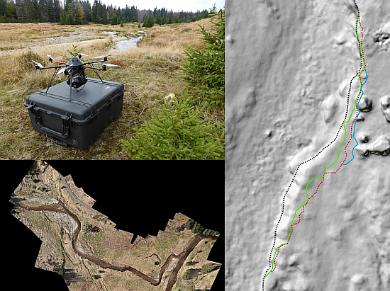
The research was focused on the experimental basin of Javoří brook, Šumava Mtns., Central Europe, as an example of a highly dynamic small montane stream that experiences repeated flooding. Repeated imaging using the UAV platform MikroKopter Hexa XL began in 2013 over a period of six months, therein separately capturing the effects of winter and summer floods. Information on the dynamics of hydro-climatic processes was acquired by an automated sensor network in the area conducting long-term operations. The accuracy and quality of data obtained from UAS imaging was compared with conventional data from aerial LiDAR scanning.

2. Material and Methods

2.1. Study Area

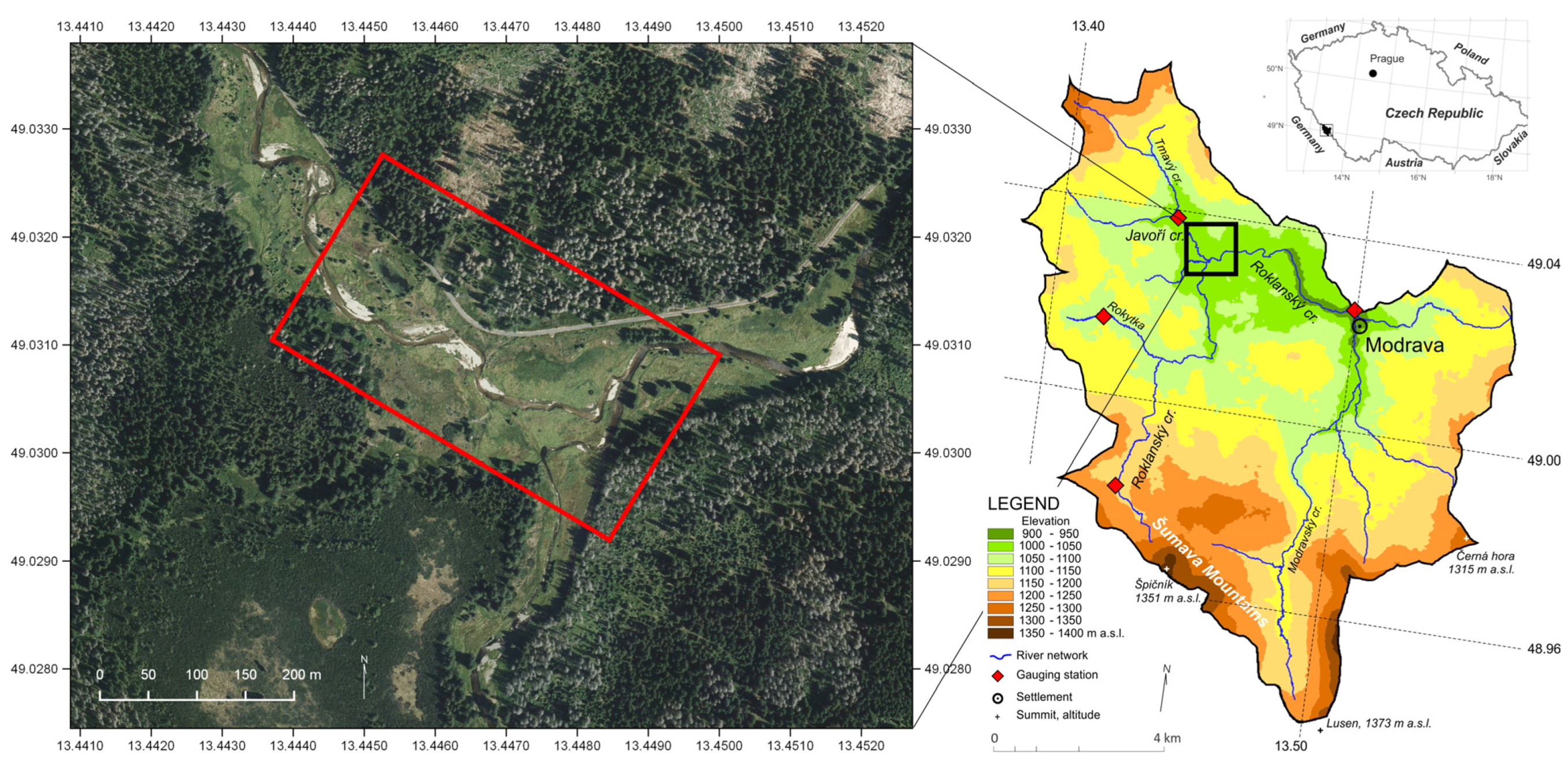
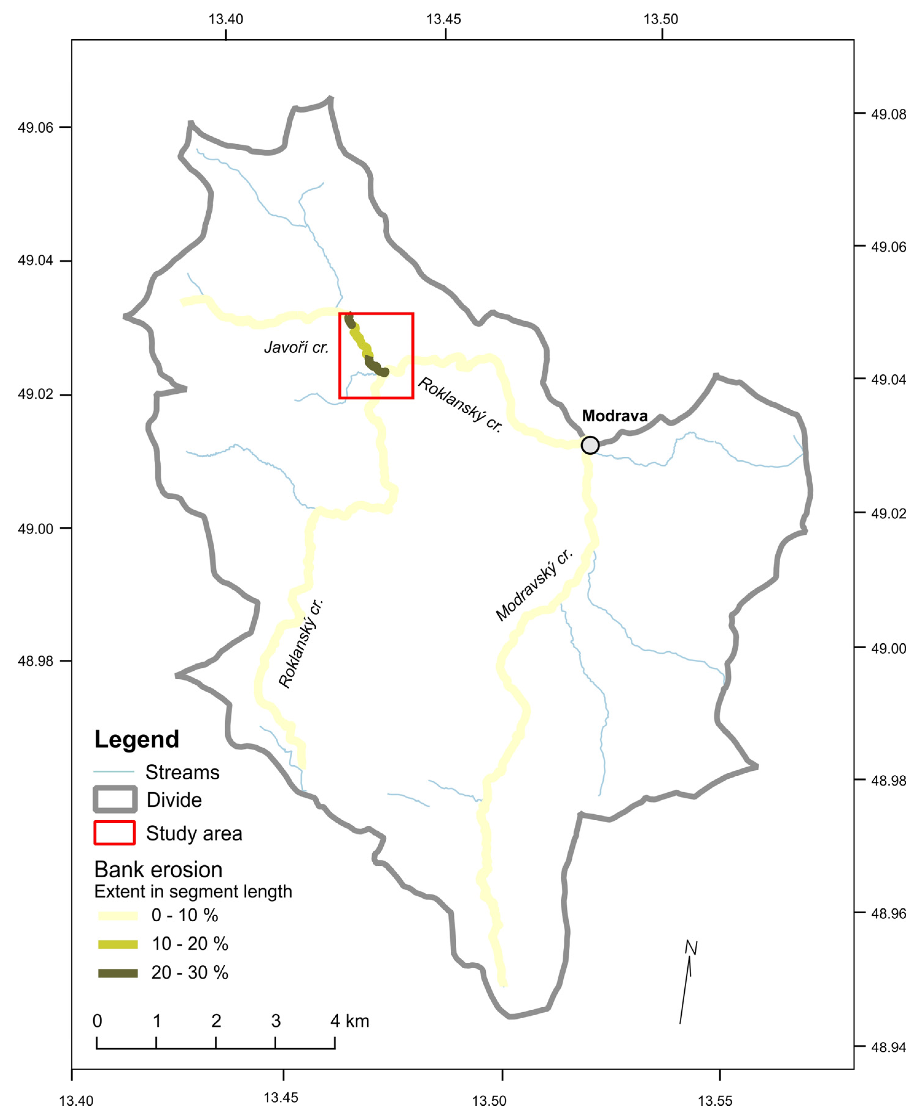
The UAS and TLS techniques were applied to the experimental catchment of the Javoří brook in the Šumava Mts., Czech Republic, Central Europe, for the analysis of recent fluvial dynamics. The study area is located in a mid-latitude montane area with an altitude of approximately 1100 m a.s.l., situated on the border between the Czech Republic and Germany (Figure 1).

Figure 1. Study area: Confluence of Javoří and Roklanský brook with marked zone of UAS imaging (left) as a part of the upper Vydra Basin (right).

Figure 1. Study area: Confluence of Javoří and Roklanský brook with marked zone of UAS imaging (left) as a part of the upper Vydra Basin (right).

The study area, located in headwaters of a montane range is experiencing frequently peak flows, generated by snowmelt in spring as well as by spring and summer storms [12,13]. This includes extreme flood events resulting from regional rains, such as in August 2002 [13], or from heavy rainstorms such as in July 2009 [14]. In addition, this area is undergoing significant changes in land use, settlement, and management practices. The mountains were covered by virgin forest until the 18th century, in which it was converted to forest spruce monoculture for the wood industry. As a result, the region is repeatedly affected by bark beetle outbreaks, which accelerate forest damage after windstorms [15] and the hydrological processes and fluvial dynamics [12].

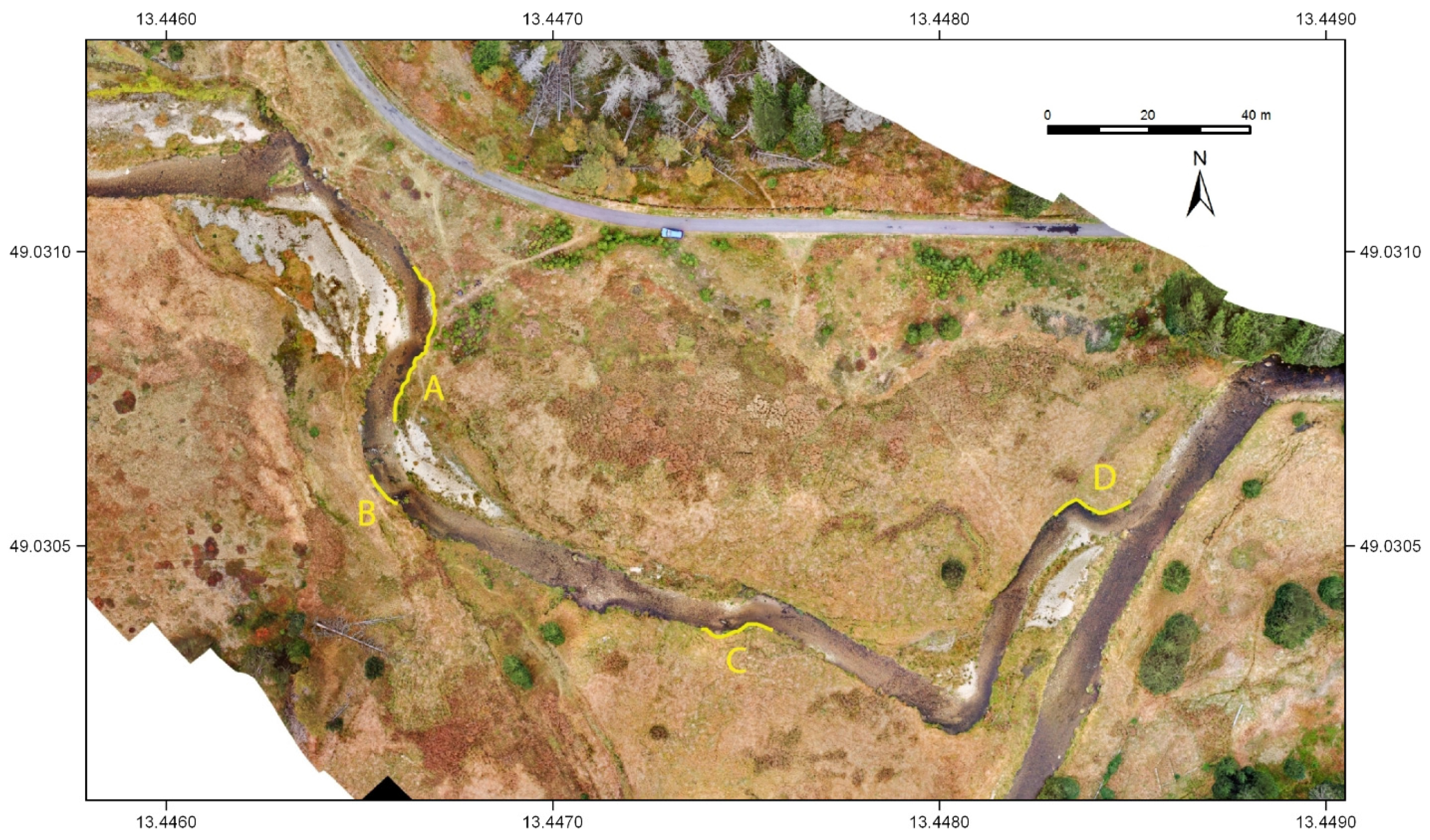
The monitoring of fluvial dynamics was focused on a zone with elevated dynamics of fluvial processes at the confluence of two streams—the Javoří and Roklanský brook. The meandering stream of the Javoří brook was, in the past 150 years, subject of modifications of the stream route resulting from high fluvial dynamics of the system as well as man-made modifications [16]. This segment of stream displayed elevated dynamics of fluvial processes in response to recent flooding in 2013, in particular, by the occurrence of bank scour and fresh fluvial accumulations in long compact segments. Because the hydromorphological mapping of the area indicated this zone as the most dynamic in the area, we have selected it as the experimental site for the monitoring of flood effects and stream channel changes using UAS photogrammetry.

Information on hydrological regimes is derived from long-term discharge monitoring and the climate station operated by CHMI in the study area. Water levels have been observed since the 1930s at the Vydra Basin outlet in Modrava, and precipitation is measured at an adjacent station at Filipova huť.

In the basin, an automated sensor network for the monitoring of rainfall-runoff processes is operated by Charles University in Prague. The monitoring networks, built in the study area in 2005, are composed of 11 automatic water level monitoring stations, 3 weather stations and a snow scale. Water level measurements are performed using two principles selected according to channel conditions—measurements based on hydrostatic pressure changes and direct measurements of the water level by an ultrasonic beam. The data are acquired in 10-minute time steps and are periodically sent via GSM signal to the server so the data are accessible online with near real-time access to observations.

The data from the automated monitoring network enable the analysis of the dynamics of runoff events and their relations to the fluvial processes at high levels of spatial and temporal detail. The distribution of gauging stations in all major streams of the basin enabled the coupling of the information of spatial and volumetric changes in streams and floodplains with accurate information on the dynamics of the hydrological processes driving the fluvial processes.

A field survey of the hydromorphological status of streams in the study area was used for the identification of zones with elevated dynamics of fluvial processes. The hydromorphological monitoring HEM [17] was used as the methodology for the field survey.

The field mapping was performed after the flood in June 2013 to capture the traces of recent fluvial activity and their distribution in the basin. The mapping covered three major streams of the fluvial system in the study area—the Modravský, Roklanský and Javoří brooks. The streams had a total length of 31.1 km and were divided into 129 stream segments varying from 80 to 440 meters, with a mean length of 231 m.

2.2. UAS Photogrammetry

2.2.1. Background Principles

The field of UAS (Unmanned Aerial System) photogrammetry is a rapidly evolving discipline that addresses methods and technologies for the acquisition of measurements, maps, digital terrain models and other products from photographic images [8,11]. The method combines benefits of the vertical aerial view of aerial photogrammetry with the advantages of close distances and high levels of image detail provided by ground photogrammetry [11].

The basic method for image orientation and calculation of the exterior orientation parameters is Structure from Motion (SfM). Fonstad [18] state that the SfM method uses images acquired from multiple viewpoints to restitute the three-dimensional geometry of an object or surface and diverges significantly from traditional photogrammetry. The main fundamental difference between SfM and classic photogrammetry is the use of a new generation of image matching algorithms, which allow for unstructured image acquisition. While classic photogrammetric methods typically rely on strips of overlapping images acquired in parallel flight lines, SfM was designed to restitute the three-dimensional geometry of buildings and objects from randomly acquired images [18]. The SfM method performs very well for oblique images as well as for classic aerial images with forward and side overlap.

The X, Y, Z coordinates are provided by very precise D-GPS systems. The tilts of the camera can be measured using a three-level system, preferably, an INS (Inertial Navigation System) or IMU (Inertial Measurement Unit) device. In some cases, the size, weight and price do not allow the use of IMU devices in the models [11], and it is thus necessary to perform the aerotriangulation without knowing the exterior orientation elements. The most commonly used method is to determine the elements of exterior orientation using Ground Control Points (GCPs) with known X, Y, and Z coordinates. The position accuracy of the GCPs is the most important factor that affects the accuracy of the final aerotriangulation. Measurements obtained using a standard GPS device or by extracting the coordinates from a map can be sufficient when working with small-scale images. However, for high-accuracy Small Format Aerial Photography (SFAP), a total station or GPS device with RTK (Real Time Kinematic) correction data has to be used to collect GCPs.

As described above, the control points are the most essential elements for the correct processing of aerial photographs. Control points serve as a basis for calculating exterior orientation parameters, and their accurate determination is critical for the further processing of the photographs. The accuracy of an automatic aerial triangulation (AAT) calculation is affected by several factors, including the measurement accuracy of the control points and their total number and distribution. The aerial triangulation result, or the determination of the exterior orientation parameters, will only be correct if all three factors are correctly considered.

The distribution of control points is crucial for the AAT result and its accuracy. Basically, a minimum of four or five symmetrically distributed points are necessary in conventional aerial photography [19]. However, what does “symmetrical” mean? According to commonly used photogrammetry rules, the points should be evenly distributed over the entire area of the photograph [20]. However, there are many ways to distribute the points. The theory of statistical estimates and solvability of linear equations suggests that the error rate of the model increases if there is a linear relation between the points [21]. Specifically, the accuracy of the result decreases. The addition of equations for a third point that is located on a line connecting two other points will not increase the rank of the matrix; consequently, this point will not increase the solvability of the system of equations; that is, this procedure will not reduce the degrees of freedom. For a distribution of points on natural terrain, the linear relation means that the points should not lie on lines. In theory, the maximum accuracy can be reached if none of the three points lie on a line.

The elements of the internal orientation can be determined either in special laboratories or by self-calibration. While aerial cameras are usually calibrated by the manufacturer, the calibration protocols for small cameras used in SFAP applications are not known. In this study, the camera calibration was performed with the PhotoModeler and iWitness software. Several types of calibration were performed, including both a single calibration grid sheet and a multi-grid calibration sheet (Table 1). The listed parameters are used only for initial processing, and the values are corrected based on the GCPs in each project.

Table 1. Interior orientation of the camera.

f (mm)	x0 (mm)	y0 (mm)	K1 (mm)	K2 (mm)	K3 (mm)
20.549	−0.142	0.152	−0.102273	0.10978	−0.040257

f - Focal Length f (mm); x₀, y₀—Principal Point X₀, Y₀ (mm); K₀, K₁, K₂—Radial Lens Distortion Coefficients

Table 1. Interior orientation of the camera.

f (mm)	x0 (mm)	y0 (mm)	K1 (mm)	K2 (mm)	K3 (mm)
20.549	−0.142	0.152	−0.102273	0.10978	−0.040257

f - Focal Length f (mm); x₀, y₀—Principal Point X₀, Y₀ (mm); K₀, K₁, K₂—Radial Lens Distortion Coefficients

Based on known exterior orientation parameters, we can reconstruct the terrain. One of the most commonly used methods is based on Semi-Global Matching (SGM) [22]. This method produces very precise dense point clouds of the surface. The method is relatively new but has a strong theoretical background from the field of computer vision [23]. Per-pixel autocorrelation matching is the basis for point cloud generation. The method successfully combines concepts of global and local stereo methods for accurate, pixel-wise matching at low runtime [24]. Many studies that compare surface or terrain created by the SGM method terrestrial or aerial LiDAR products have been published. Colomina and Molina [25] describes that the accuracy of the model is 0.5 GSD (Ground Sample Distance) horizontally and 1.5 GSD vertically. The accuracy when compared to DSM (Digital Surface Model) based on the SGM method with LiDAR-based DSM is also very good and the RMS difference is only 1 GSD [25].

2.2.2. Setting of Imaging Parameters

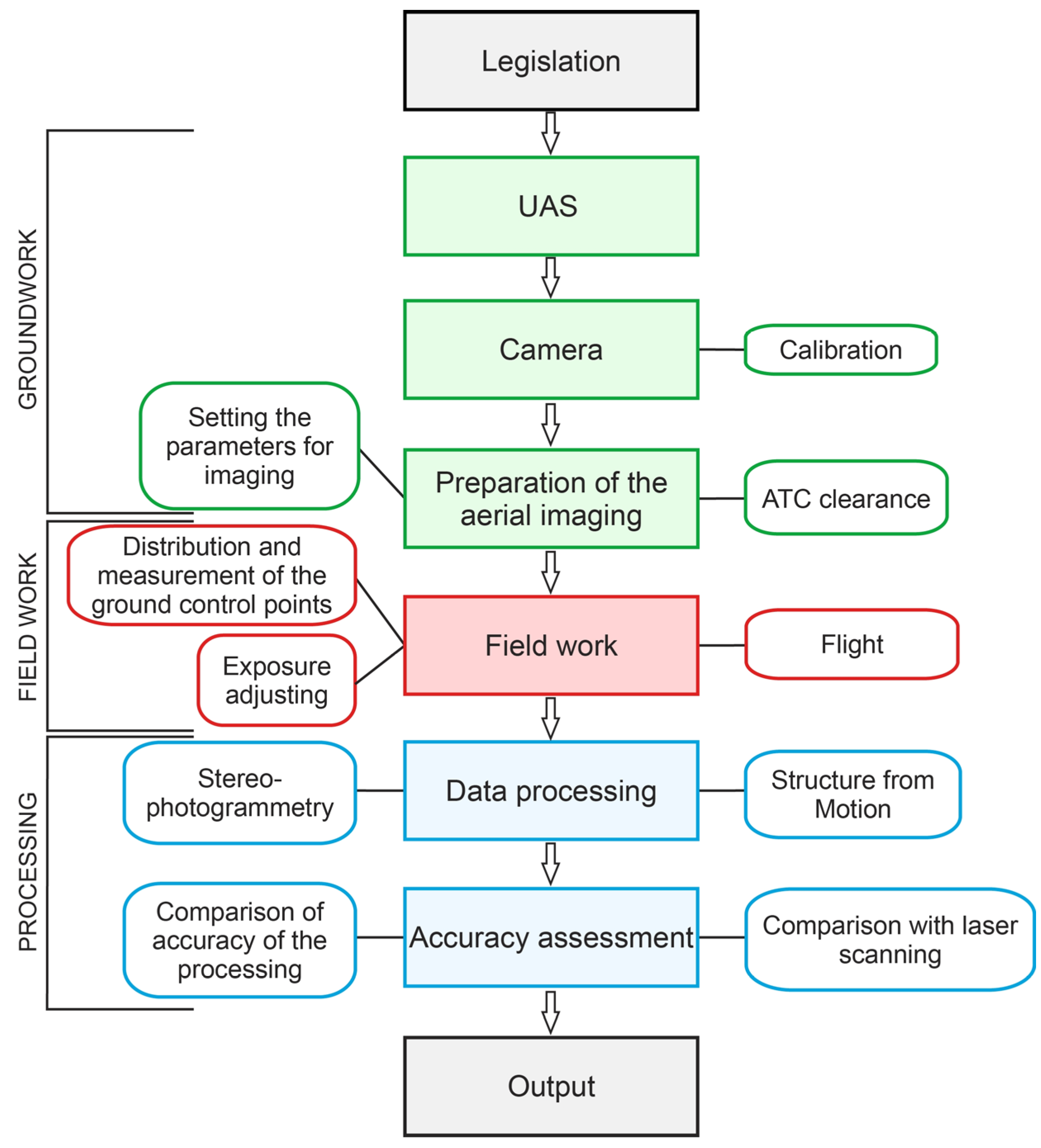
The basis for the UAS photogrammetric analysis is a series of repeated aerial flights over the same study area. In our study, the aerial imaging campaigns were designed to capture the study area twice a year. Preparation of the aerial flights and image processing corresponded to the scheme in Figure 2.

Figure 2. Workflow diagram of the aerial imaging process.

Figure 2. Workflow diagram of the aerial imaging process.

Each imaging campaign has to be correctly prepared before the flight. We can distinguish two parts of the aerial planning—analytical, setting the parameters for imaging and operational, setting up the flight route plan.

The most important parameters of the analytical part are the flying height, focal length of the camera, image scale, distance between two points where the image is taken and GSD (Ground Sample Distance). First, we have to specify the required GSD. We decided that for our all-aerial imaging, the GSD should not exceed 2.2 cm. Based on the known basic input parameters (GSD, focal length of the lens and sensor size of the camera), the characteristics of the flight and imaging were calculated—the average values of flight altitude, image scale, area coverage per image and the distance of exposure points ensuring imagery overlaps. The resulting imagery characteristics, applied for the design of the imaging campaign are listed in the Table 2, the calculation of parameters is described in detail in Appendix.

Table 2. Calculated parameters of imaging.

Parameter	Value
f—focal length (mm)	20.5
p—real size of the sensor (mm)	22.33 × 14.89
Hg—average flying height (m)	97
GSD—Ground Sample Distance (mm)	22
M—image scale	1:4663
PE—Overlap of the image in percent (%)	80
B—distance between two exposure points (m)	20.8

Table 2. Calculated parameters of imaging.

Parameter	Value
f—focal length (mm)	20.5
p—real size of the sensor (mm)	22.33 × 14.89
Hg—average flying height (m)	97
GSD—Ground Sample Distance (mm)	22
M—image scale	1:4663
PE—Overlap of the image in percent (%)	80
B—distance between two exposure points (m)	20.8

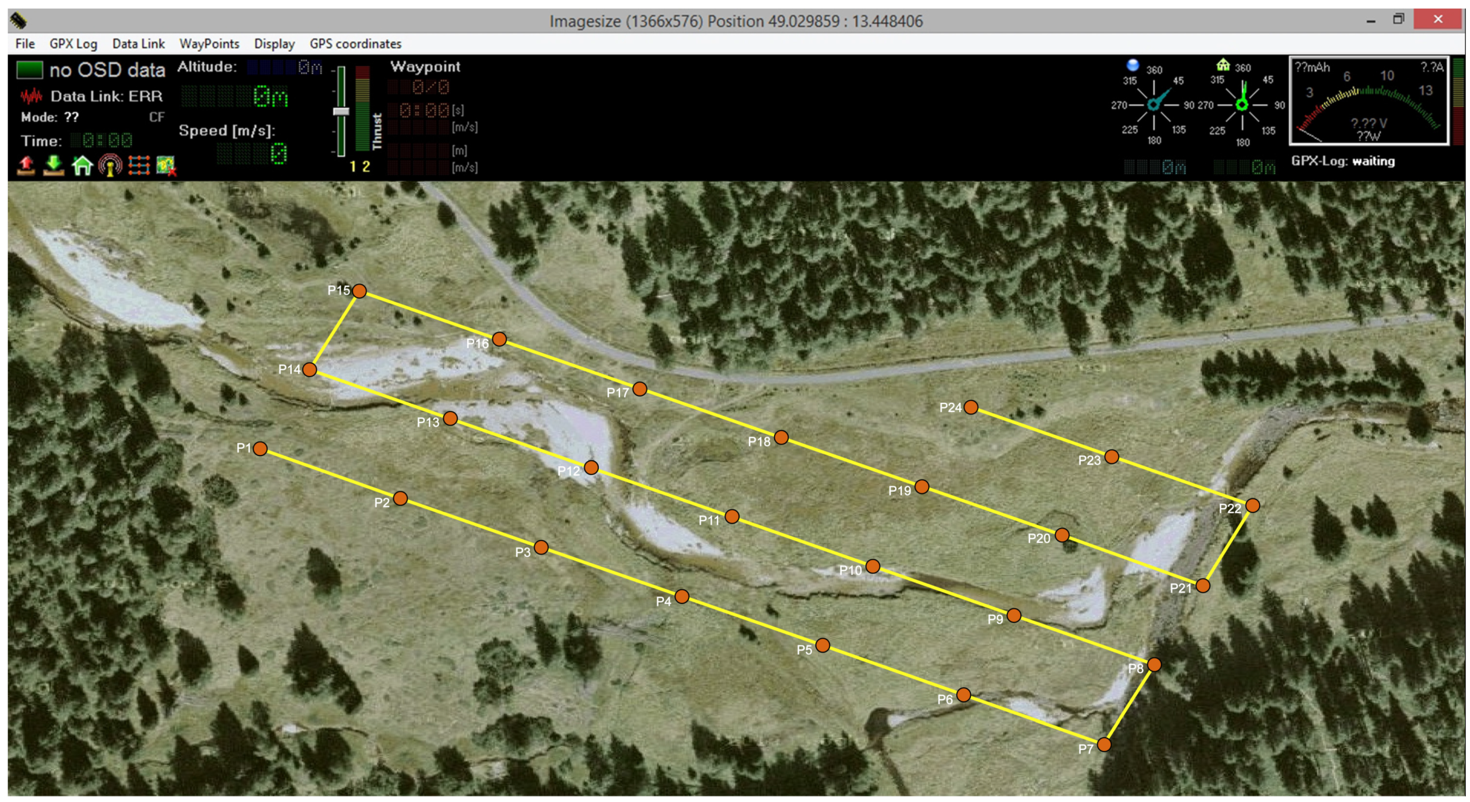
The operational part of imaging preparation is as important as the analytical part because it is used to design the flight route in the form of flight lines and waypoints. The unmanned aircraft then flies along these lines and captures the images. Such a flight route can be of benefit to repeated imaging campaigns to ensure comparable conditions for the acquisition of imagery (Figure 3).

Figure 3. Graphical interface of the flight planning software with highlighted flight lines and waypoints. Screenshot from MikroKopter flight planning tool.

Figure 3. Graphical interface of the flight planning software with highlighted flight lines and waypoints. Screenshot from MikroKopter flight planning tool.

2.3. Design of Monitoring Campaign

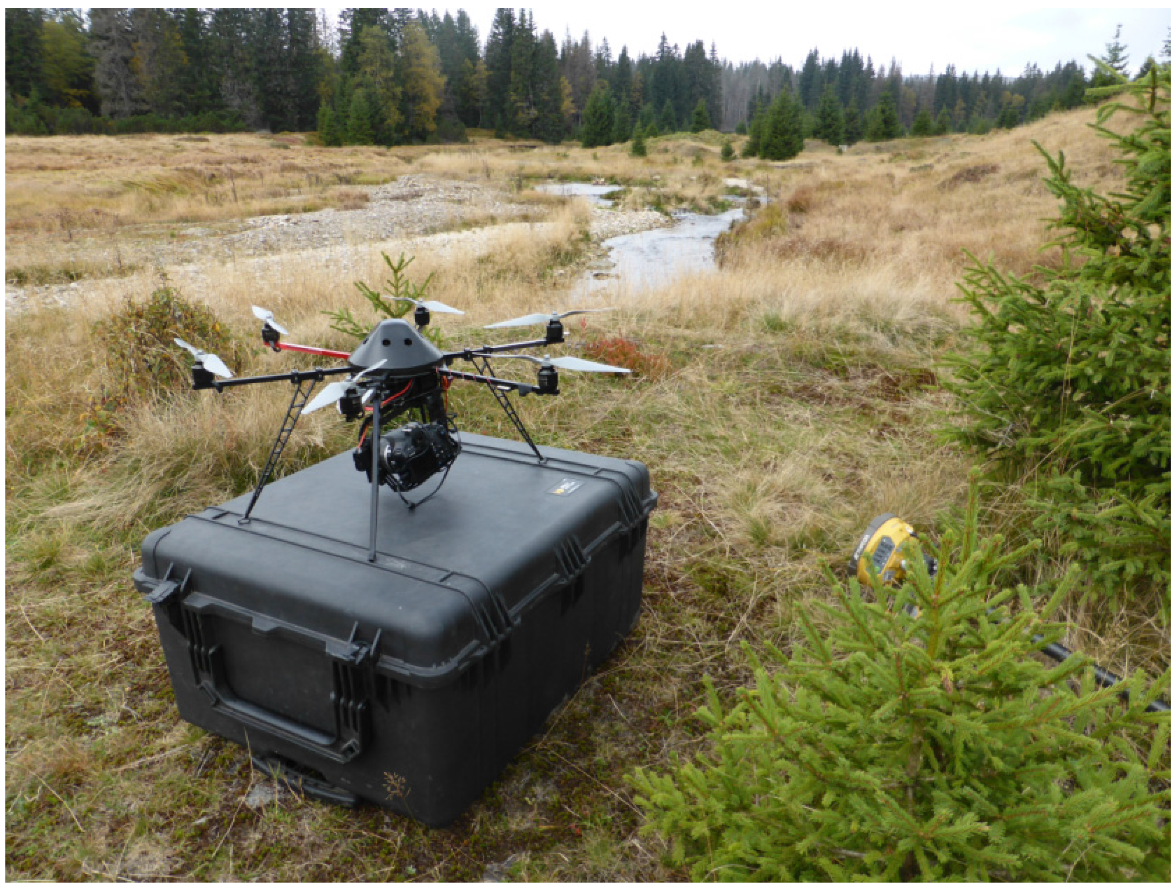
For the aerial imaging, we used the Hexacopter XL aircraft. It is a multi-rotor platform equipped with six propellers and maximum payload of 1.5 kg (Table 3). The imagery was taken using a Canon EOS 500 D camera and special calibrated lens with a fixed focal length of 20 mm (Figure 4 and Table 3).

Figure 4. UAS Mikrokopter Hexa XL with Canon EOS 500D camera, used for UAS imaging in the study area of the Javoří brook. Photo J. Langhammer, 2014.

Figure 4. UAS Mikrokopter Hexa XL with Canon EOS 500D camera, used for UAS imaging in the study area of the Javoří brook. Photo J. Langhammer, 2014.

Table 3. Technical specifications of the Hexacopter XL UAS platform.

Technical specifications—Hexacopter
Action range	1 km
Flight Altitude	5–500 m
Flight speed	0–20 km/h
Flight time	Up to 30 min.
Maximum operational wind speed	0–30 km/h
Engine	Electric
Weight without battery	1.5 kg
Payload capacity	up to 1.5 kg

Table 3. Technical specifications of the Hexacopter XL UAS platform.

Technical specifications—Hexacopter
Action range	1 km
Flight Altitude	5–500 m
Flight speed	0–20 km/h
Flight time	Up to 30 min.
Maximum operational wind speed	0–30 km/h
Engine	Electric
Weight without battery	1.5 kg
Payload capacity	up to 1.5 kg

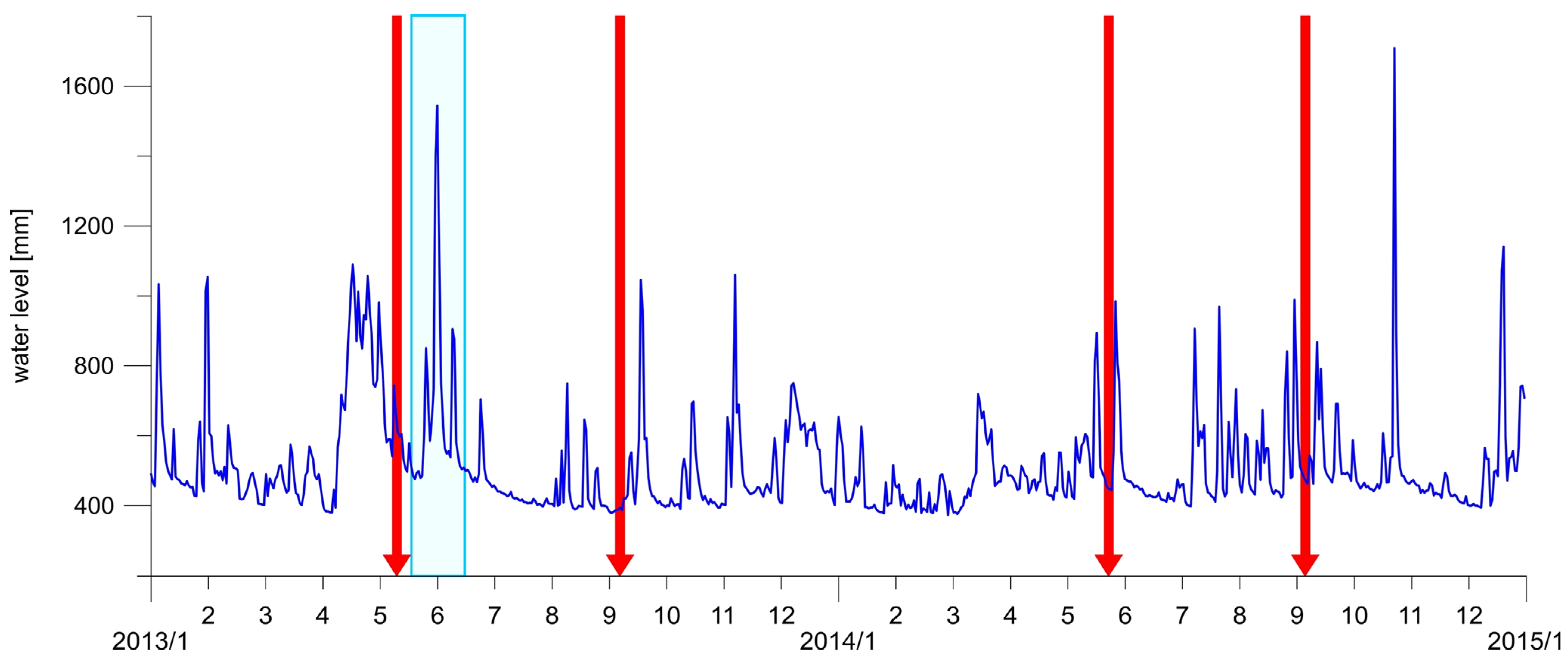
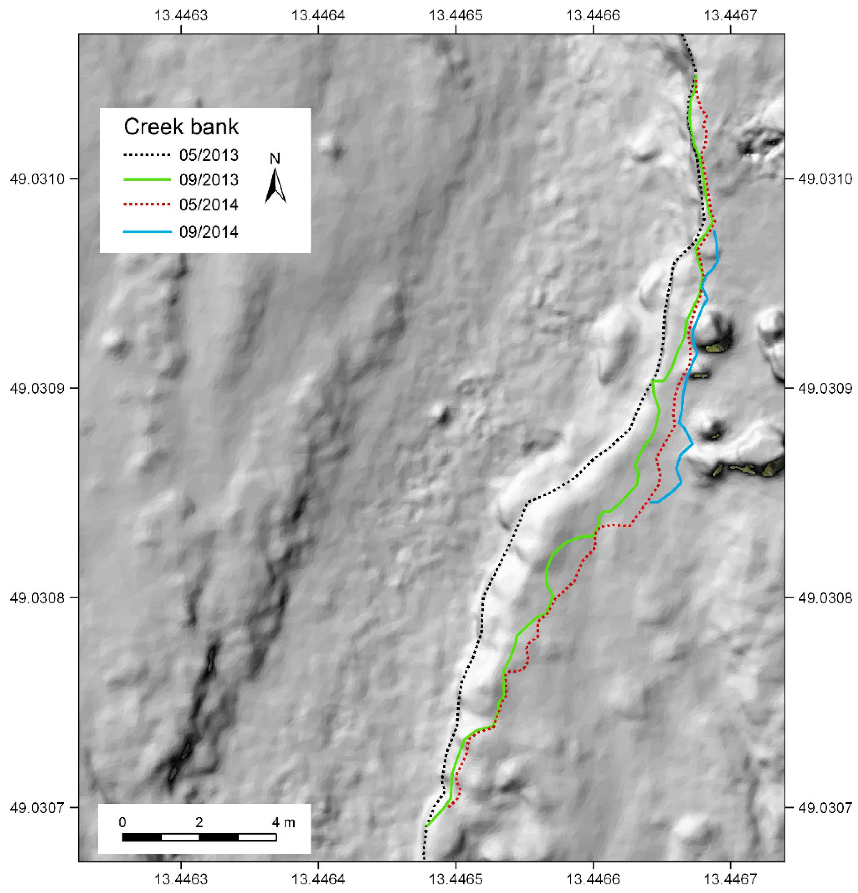
The monitoring campaign was designed to enable the capture of changes in the fluvial geomorphology of the stream resulting from peak flows in the summer and winter seasons (Figure 5). The initial imaging was performed in May 2013 prior to the flood event in June 2013, which triggered the extensive morphological changes in the assessed stream channel. The consequent imaging campaigns was designed to cover two different periods of changes of fluvial geomorphology in area. First is in May and covers changes after winter period and spring peak flows generated by snowmelt, occurring in the area typically in April. Second period of imaging was set to September, covering the effects of peak flows generated from spring and summer storms and regional rains. The applied dataset is created using four sets of imagery, taken in May 2013, September 2013, May 2014 and September 2014, using the same platform, with similar camera and flight parameters (Table 2).

For each flight, there were 21–33 ground control points (GCP, Table 4) located at locations with no displacements. The positions of GCPs was measured during each monitoring campaign immediately prior the imaging to ensure coincidence of positioning and imaging. High-precision GNSS system with RTK corrections (Topcon HiPER II) was used with a horizontal precision of 1–3 cm and vertical precision of 2–5 cm at each point. We used three seconds observation for each GCP and checkpoint during RTK positioning as the standard, recommended by the Czech State Administration of Land Surveying and Cadastre authority. For RTK corrections we have used Virtual Reference Station (VRS) located five kilometers from the area of interest. The VRS is calculated based on the real reference stations from the private or national permanent GNSS reference stations.

Table 4. Parameters of the imaging flight and image processing.

May 2013	Value	September 2013	Value
Number of images	41	Number of images	78
Flying altitude (m)	87.5	Flying altitude (m)	103
Ground sample distance (cm)	1.9	Ground sample distance (cm)	2.3
Number of ground control points	33	Number of ground control points	23
Image coordinate error (pix)	0.67	Image coordinate error (pix)	0.76
Point density (points/m2)	201	Point density (points/m2)	221
Standard deviation (m)	0.027	Standard deviation (m)	0.031
RMSEZ (m)	0,020	RMSEZ (m)	0.031
May 2014	Value	September 2014	Value
Number of images	107	Number of images	86
Flying altitude (m)	101.5	Flying altitude (m)	105
Ground sample distance (cm)	2.1	Ground sample distance (cm)	2.2
Number of ground control points	21	Number of ground control points	21
Image coordinate error (pix)	0.66	Image coordinate error (pix)	0.55
Point density (points/m2)	130	Point density (points/m2)	139
Standard deviation (m)	0.032	Standard deviation (m)	0.030
RMSEZ (m)	0.037	RMSEZ (m)	0.037

Table 4. Parameters of the imaging flight and image processing.

May 2013	Value	September 2013	Value
Number of images	41	Number of images	78
Flying altitude (m)	87.5	Flying altitude (m)	103
Ground sample distance (cm)	1.9	Ground sample distance (cm)	2.3
Number of ground control points	33	Number of ground control points	23
Image coordinate error (pix)	0.67	Image coordinate error (pix)	0.76
Point density (points/m2)	201	Point density (points/m2)	221
Standard deviation (m)	0.027	Standard deviation (m)	0.031
RMSEZ (m)	0,020	RMSEZ (m)	0.031
May 2014	Value	September 2014	Value
Number of images	107	Number of images	86
Flying altitude (m)	101.5	Flying altitude (m)	105
Ground sample distance (cm)	2.1	Ground sample distance (cm)	2.2
Number of ground control points	21	Number of ground control points	21
Image coordinate error (pix)	0.66	Image coordinate error (pix)	0.55
Point density (points/m2)	130	Point density (points/m2)	139
Standard deviation (m)	0.032	Standard deviation (m)	0.030
RMSEZ (m)	0.037	RMSEZ (m)	0.037

3. Results

3.1. Dynamics of Hydrological and Fluvial Processes in the Study Area

The hydrological regime of the upper Vydra Basin up to the Modrava station has properties of a typical mid-latitude montane basin. The seasonal distribution of runoff is dominated by the spring snowmelt, which typically occurs in April–May [12]. However, the most significant runoff events are caused by precipitation. In the assessed time period of 2013–2014, nine peak flows were recorded as exceeding the level of a one-year flood. The observed runoff dynamics of the Roklanský brook during the assessed period (Figure 5) is typical based on the high frequency of low-magnitude peak flows with a dominant spring season.

Figure 5. Dynamics of hydrological regime of Roklanský brook. Daily average water levels in the period 2013–2014 with highlighted terms of UAV imaging (red arrows) and period of flood event in June 2013 (light blue box). Data: Charles University in Prague.

Figure 5. Dynamics of hydrological regime of Roklanský brook. Daily average water levels in the period 2013–2014 with highlighted terms of UAV imaging (red arrows) and period of flood event in June 2013 (light blue box). Data: Charles University in Prague.

The peak flow events driven by summer rainstorms are of very short duration with steep rising and recessing limbs. The initial flood event (Figure 5), triggering the observed fluvial processes, occurred in June 2013, with a magnitude corresponding to a 2–5-year flood. This flood resulted from the recurrent heavy rainfalls coming to the basin, which was previously saturated by snowmelt [26].

The analysis of the spatial distribution of fresh fluvial accumulations and of the bank erosion revealed high concentrations of evidence of the recent fluvial activity into a limited zone of the stream system downstream of the Javoří brook near the confluence with the Roklanský brook. In this zone, all of the stream segments are concentrated, with significant evidence of bank erosion. All evidence of bank erosion resulting from the 2013 spring flood is located in a 2-km-long stretch of the Javoří brook between the confluence of the Tmavý and Roklanský brook (Figure 6). This stream segment of channel width 5–7 m was selected for a further multitemporal analysis of the dynamics of the fluvial processes using UAS photogrammetry.

3.2. UAS Data Acquisition and Processing

The imaging was performed in May 2013, September 2013, May 2014 and September 2014. The images were photogrammetrically processed using Structure from Motion (SfM) and Semi-Global Matching (SGM) methods. A morphometric analysis of the development of the brook was performed based on the processed images. The parameters of the imaging flights and resulting image processing are listed in the Table 4.

Figure 6. Spatial distribution of evidence of bank erosion resulting from flooding in 2013 based on field mapping of the hydromorphological status of streams. Data: Charles University in Prague, 2013.

Figure 6. Spatial distribution of evidence of bank erosion resulting from flooding in 2013 based on field mapping of the hydromorphological status of streams. Data: Charles University in Prague, 2013.

The flight altitude was in all cases approximately 100 m above ground level, varying from 87.5 to 105 m (Table 4). The ground sample distance (GSD), a key parameter of the spatial resolution, was approximately 2 cm (1.9 to 2.3 cm). The most important parameter in the image processing is the RMSE, and the worst obtained value is 3.7 cm. The RMSE error as well as standard deviation was calculated based on five checkpoints, which were not used in the transformation. These points were measured using geodetic RTK method. Then, we compared the coordinates (X, Y, Z) of these points with the coordinates calculated using the SfM method.

The achieved resolution and reliability of the imagery suggest its good applicability for analysis in fluvial geomorphology. The GSD of 2 cm enables researchers to distinguish even the fine details of the stream channels, to identify individual stones with sizes down to approximately 8 cm and to track changes at such levels of detail over time.

Digital Surface Model and Orthoimage Mosaic

Two of the most important results are the digital surface model (DSM) and digital terrain model (DTM). If we know the exterior orientation parameters of the images, we can calculate the model based on the Semi-Global Matching (SGM) method. The use of the DTM or DSM is important for image orthogonalization.

The digital terrain model is created based on the acquired UAS imagery. The terrain model, created using the SGM method, can be very precise but still remains to be converted into a digital surface model. To obtain the DSM, we have to classify it mathematically according to the following steps:

• To choose the right cell size, the lowest point is found in each cell.
• Other points are classified from this point based on specified parameters.
• The parameters are the following: maximum angle between lowest and classified point and maximal distance between the lowest and classified point.
• If the classified point exceeds the given parameters, then it is excluded from the point cloud.

Figure 7 shows the final raster with hill shading. The left image demonstrates the digital terrain model, and the right picture provides further details. This terrain model was created following the point cloud classification based on our criteria.

Figure 7. Digital terrain model of the study area resulting from an aerial imaging (May 2013).

Figure 7. Digital terrain model of the study area resulting from an aerial imaging (May 2013).

Orthorectification and mosaicking of the images are the final processes of the photogrammetric workflow. Orthorectification was done in Erdas IMAGINE (LPS toolbox). Final mosaic was created in Trimble OrthoVista. These datasets form the basis for the subsequent spatial-temporal analysis.

3.3. Spatiotemporal Analysis

Long-term monitoring and aerial imaging with high spatial resolution offer good opportunities for analysis and spatial-temporal analysis. We have analyzed four datasets from two years. Figure 8 shows the study site of the Javoří brook in the initial status of surveying in May 2013. UAS imaging facilitated the identification of the details of the stream channel and floodplain, which are necessary for the analysis of changes in fluvial geomorphology.

Based on the field survey in September 2013, we have identified stream segments with active lateral erosion. Quantitative measurement of the lateral erosion was done in ArcGIS for Desktop 10.1. The channel banks were digitized and the distance between them was measured. The distance was measured in regular step (each two meters) extended by the points with minimal and maximal differences. The measurement line was always perpendicular to the given section. Four segments marked A–D, where the effect of initial event was apparent in the change of bank line in the acquired imagery, were subject of further tracking. Across the series of four imaging campaigns over two years the highest extent of bank erosion was detected in segments A and D and these two segments thus were selected for quantitative analysis (Figure 8).

Figure 8. Orthomosaic and lateral erosion of Javoří brook with identification of spots of the lateral erosion.

Figure 8. Orthomosaic and lateral erosion of Javoří brook with identification of spots of the lateral erosion.

By far, the most extensive changes after the flood in June 2013 were detected in segment A, representing the outer bank of the first meander in the investigated system. In this segment, the fluvial processes were active over the whole assessed period. In contrast, the changes in segments B–D were single instances. In addition to the direct effects of the flood in June 2013, as apparent in the changes between May and September 2013, the extent of bank erosion in these segments was negligible.

The progress and extent of bank erosion thus was further tracked in segments A and D. The orthoimage and 3D models resulting from the UAS imaging were used to analyze the lateral movement of the bank line, areal extent of the changes and volumetric changes in these segments over the assessed period.

3.3.1. Lateral Movement of Channel Bank

Multitemporal analysis of the changing positions of the bank line based on UAS orthoimages revealed the extent and evolution of changes in segment A. The maximum difference of the bank line in the stream, with an average width of six meters, reached more than two meters at this location (Figure 9). The greatest change resulted from the initial flood in June 2013, when the lateral movement of the bank line reached 1.5 meters. The changes in consequent periods were less intense in terms of the change in the maximal shift of the bank line. However, in the follow-up period, the bank erosion was almost as high as the length of the meander bend. The last assessed period over summer 2014 resulted in minor changes, located mostly in the front part of the meander (Figure 9).

Figure 9. Evolution of lateral erosion at the most active zone in the segment A.

Figure 9. Evolution of lateral erosion at the most active zone in the segment A.

Differences in the response of the fluvial activity of the two assessed segments at different positions in the meandering system are apparent when comparing the quantitative aspects of the changes, in particular, the areal and volumetric changes.

The cumulative extent of the area cut by the bank erosion (Figure 10a) indicates that for both segments A and D, the decisive changes resulted from the first flood event.

The intensity of the changes in the first period (May–September 2013) is comparable in both segments. In segment A, the areal loss in the 20-m-long segment reached 10 sq. m, and in segment D, which has a total length of 14 meters, the initial change reached 6.7 m².

However, the difference between the two segments is apparent from further multitemporal evaluation. Since the flood in June 2013, segment A, located at the outer band at the entrance to the meandering system, remains bare and experiences permanent fluvial activity. The extent of area, cut by the bank erosion, is continuously increasing and since September 2013 has almost doubled compared to the initial period of change.

In contrast, the fluvial activity in segment D, located at the end of the assessed meandering system, has been mitigated. The bank becomes grassed and stabilized, and thus, the further extent of areal change since September 2013 is negligible.

Figure 10. Cumulative erosion rate at segments A and D. (a) Accumulated area change; (b) Accumulated volumetric change.

Figure 10. Cumulative erosion rate at segments A and D. (a) Accumulated area change; (b) Accumulated volumetric change.

3.3.2. Volumetric Changes

Based on the 3D DTM derived from the UAS imagery, we calculated the volumetric changes for both assessed segments. Because the imagery was acquired under different water levels, the calculation of volumes in the submerged zone suffers from large uncertainties. The volumes were thus calculated as the volume above the applied reference plane and cropped to the same extent in the upper part of the bank. The reference plane was set based on the highest water level from all images at 1016.3 m above MSL (Figure 11).

From the multi-temporal analysis of the pairs of DTMs derived from the UAS imagery, the volume of material cut by the bank erosion in the assessed periods was derived. In segment A, there is an apparent continuing loss of material even over the next year after the initial flood. In total, the lateral erosion in the 20-m-long segment caused 3.46 m³ of the soil to be removed and subject to transport down the stream.

The spatial extent of bank erosion in segment A continued to propagate continuously over the following periods. The volumetric changes were discontinued after the first year since the flood, and there is no significant change between May and September 2014 as a result of the incipient stabilization of the bank (Figure 10b).

Figure 11. Visualization of 3D model of segment A. Left—May 2013; Right—September 2014.

Figure 11. Visualization of 3D model of segment A. Left—May 2013; Right—September 2014.

The volumetric changes evolve differently compared to the areal changes. While the largest areal change occurred immediately after the initial flood event, the largest volume of material was cut off in the period following the first period of the post-flood changes (Table 5). Based on the methodology in [9], we have calculated RMS error between each pair of two digital surface models based on three stable areas. The maximum calculated error is 5 cm, which corresponds to the precision of the RTK method. As a second step we have calculated differences at the stable parts of the bank top between each pair of datasets included in volumetric analysis. Sum of these errors expresses uncertainty, which must be taken into consideration in the assessment of volumetric changes.

Table 5. Progress of bank erosion between 2013 and 2014 in the selected area.

Locality	Parameter	May 2013–September 2013	September 2013–May 2014	May 2014–September 2014
Segment A	Cut off area (m2)	10.2	3.6	3.7
	Volumetric changes (m3)	3.46	4.23	0
	Total error (m3)	0.39
Segment D	Cut off area (m2)	6.69	1.13	0
	Volumetric changes (m3)	4.81	2.28	0
	Total error (m3)	0.32
RMSE (cm)		3.4	5.0	4.7

Table 5. Progress of bank erosion between 2013 and 2014 in the selected area.

Locality	Parameter	May 2013–September 2013	September 2013–May 2014	May 2014–September 2014
Segment A	Cut off area (m2)	10.2	3.6	3.7
	Volumetric changes (m3)	3.46	4.23	0
	Total error (m3)	0.39
Segment D	Cut off area (m2)	6.69	1.13	0
	Volumetric changes (m3)	4.81	2.28	0
	Total error (m3)	0.32
RMSE (cm)		3.4	5.0	4.7

4. Discussion

4.1. Accuracy of UAS-Derived Data

The research in the Šumava Mts. and around the Roklanský brook uses very accurate spatial data that are based on the Structure from Motion methods and unmanned aerial systems. The precision of the results, however, must be tested. The resulting RMSEs indicate that accuracy of the acquired datasets enables their application for analysis of river channel changes of small streams, where the high level of spatial detail is required. Similar results are shown in [18]. This study compared results of a 3D model created using laser scanning and the 3D model created from aerial images of the Pedernales River, Texas, USA. The mean error in the Z coordinate is 0.07 m for the aerial photogrammetry method and 0.51 m for the LiDAR measurements. The accuracy achieved by the UAS in this study is very close to our results for Roklanský brook. We can also compare our results with a similar study by Flener et al. [2] by analyzing changes on a riverbank based on a combination of a UAV system and a terrestrial laser scanner. The authors obtained very precise 3D model and orthomosaics. The precession of their result is better than 10 cm in the Z coordinate. If we focus on the results obtained by the terrestrial laser system, we can see that the RMSE is better than 2 cm. The combination of these two methods is efficient but applicable only for small areas. Other studies apply analogous imaging and photogrammetric principles to obtain solutions of different tasks with similar findings on spatial resolution and accuracy of the UAS-based datasets [9]. The authors in [9] used error estimation of two DSMs based on the RMSE. They applied the offset of the model based on this error as the second step. We have applied this methodology in the next step to estimate the total error of the models. In our study, the RMSE was not higher than 5 cm. This value is generally low and it corresponds with range of precision of the RTK method. However, in our study we have not applied the general offset due to the high spatial variability of the error values across the DTM.

Very precise orthophoto mosaics with 2 cm spatial resolution have been, e.g., used for the evaluation of soil erosion. Sládek and Rusnák [27] used 67 images to create a 3D model of one part of the Morava River. Miřijovský, et al. [8] addressed a very precise analysis of the river bank changes in the Litovelské Pomoraví natural preserve (Czech Republic). In the above-mentioned studies, when applying generally available hardware (DSLR cameras, commercial multi-rotor platforms and common software tools), the achieved precision of the datasets created using UAS is also on the order of centimeters.

4.2. Applicability of UAS Data in Fluvial Geomorphology

Remotely sensed data, such as terrestrial LiDAR or UAV photogrammetry, can significantly improve the accuracy and reliability of assessments in fluvial geomorphology conducted at small scales, where a high topographical resolution is required. When performing manual mapping to obtain the significant terrain schematization, errors can arise from subjective observations and evaluation of key flow patterns and also from the flow pattern variations at different water stages [1]. The field mapping procedure is also very time consuming and requires powerful equipment and qualified approaches based on combined geodetic and hydroinformatic knowledge. Remote sensing can provide detailed surface descriptions, but the channel bed information crucial for obtaining a correct hydrodynamic model description is missing.

The channel morphology determines the flow dynamics [3,28] and vice versa. It is expected that the channel morphology can be derived from the observed flow dynamics [1] mainly using the velocity field and stream power identifications. In the regions with slow flow, a pool with an above average depth can be expected, and the fastest flows are observed at steps and shallow reaches. Thus, several studies were conducted to determine bed morphology from the water surface slope or longitudinal profile of talweg [29].

The most frequent, and most likely the most reliable, approach is the fusion of the model from remote sensing with the submerged zone bathymetry achieved via surveying. Among the methods used for bathymetry surveys, the most precise information can be obtained by geodetic measurements using all stations or using the geodetic GNSS positioning along cross sections and important break lines of bed structures [30]. Such bathymetry can be represented by regular grids or by TIN schematization, which may bring more accurate results in small natural channels where the flow dynamics are predetermined by the step-pool pattern [31].

4.3. Applicability of UAS Data for Tracking Flood Effects

UAS technologies represent a significant shift in natural hazards research and management, where the rapid acquisition and treatment of precise spatial information is of great importance. Namely, floods and landslides are examples of natural hazards where precise and up-to date spatial information is of great importance. The spatial information is needed here for the assessment of the course and extent of the given event, assessment and interpretation of its aftermath and as a source for analysis, modeling and prediction of its behavior.

One of the key benefits of the UAS technology, in addition to the above-discussed precision, is the high operability of imagery acquisition. UAS imaging allows the frequent limits in terms of the accessibility of the affected areas to be overcome and repeated surveys to be performed to track the course of an event or its effects. Using the programmable flight tracks and parameters improves the efficiency of repeated imaging for building multi-temporal datasets. It allows flights with the same properties, including the flight route, waypoints, flight altitude, imaging locations or frequency, to be repeated. This approach secures appropriate coverage of the zone of interest, increases the comparability of the time slices for imaging and reduces the time for operation, which, in the case of natural hazards, is an important factor. The rapid mapping of flood effects in streams and floodplains, capturing the actual state and tracking the changes from a multitemporal perspective are examples of key products for research as well as for the decision-making process that UAS technologies may offer. For remote or uncovered areas or a small stream, such as the example in the article, UASs may be the sole source of spatial information, thus enabling the necessary data to be quickly created from scratch with adequate precision and reliability.

5. Conclusions

This paper explores the potential of UAS photogrammetry for monitoring fluvial processes driven by floods in a mid-mountain environment of the upper Vydra Basin, Šumava Mountains, Central Europe. The multitemporal analysis is based on four data collections of aerial imagery using a UAS over two years.

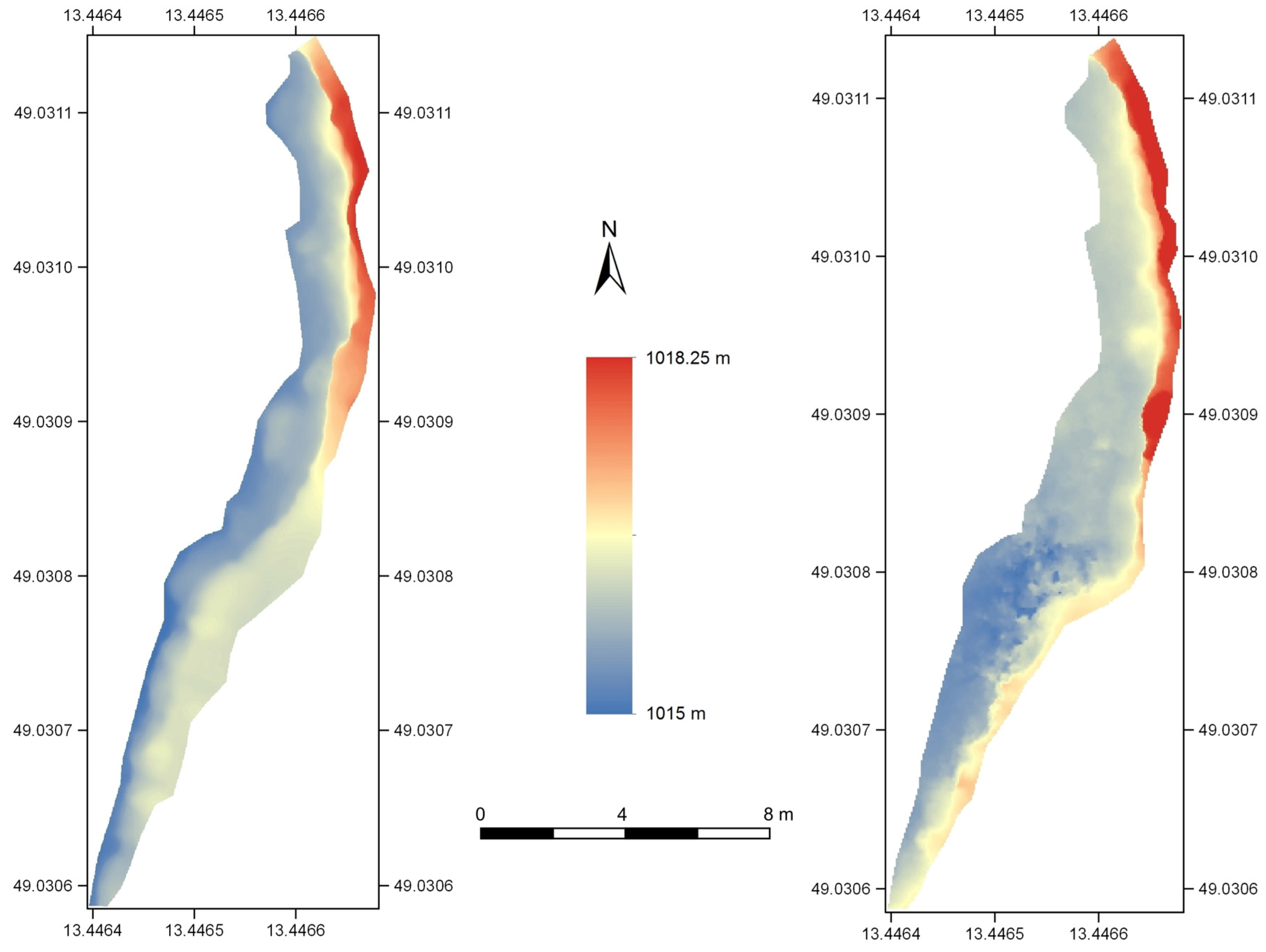
The UAS platform Mikrokopter with a calibrated camera provided aerial imaging of changes in stream channels and riparian zones in four series from May 2013 to September 2014 to track the changes in stream channels initiated by a flood in June 2013. The UAS imaging provided two basic data products for each time slice—the orthoimage and DEM. The DEM, with a resolution of 2 cm per pixel, enabled identification and analysis of changes in the stream channel at high levels of detail in addition to the quantitative analysis of changes in stream–channel planform, aerial extent and volumetric changes in bank erosion.

Multitemporal analysis of the stream channel changes demonstrated the potential of UAS photogrammetry for analyzing all of the key aspects of fluvial dynamics at a high spatial resolution. The resolution of 2 cm per pixel at 90 meter flight altitude enables changes in fluvial forms to be detected with a precision that is higher than typical detailed field surveys and conventional data sources. The spatial resolution and accuracy of the results obtained using general equipment (consumer DSLR camera and commercial multi-rotor platform) was able to provide DEMs with a sufficiently high accuracy adequate for application in fluvial geomorphology with a reproducibility of results suitable for multi-temporal analyses.

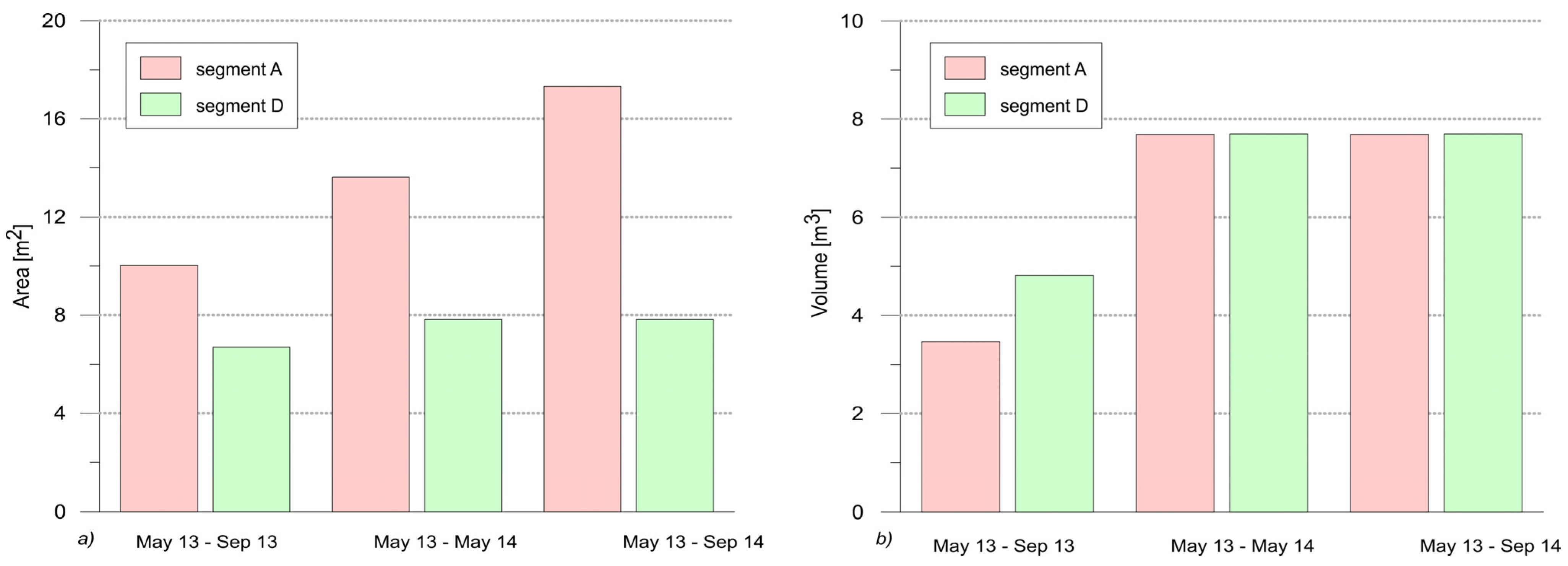
The quantitative analysis enabled areal changes by bank erosion as well as volumes of material carried away from the stream bank to be calculated for each time step. With the given resolution of 2 cm per pixel, the UAS imagery allowed individual objects, e.g., clasts or stones with size of 8 cm, to be identified and located over the entire complex scene.

The UAS-based monitoring of stream channel changes and evolution over two years since the initial flood event demonstrates the full potential of the technology for fluvial geomorphology. The multi-temporal analysis based on the UAS imagery allowed even subtle changes in stream channel and fluvial forms to be captured. The changes in the stream channel are captured in a complex manner. The maximum extent of the displacement of meandering channel drift was 2.5 meters, which represents approximately 40% of the channel width. However, the UAS imagery enables the changes in the entire stream bank line to be accurately tracked with a resolution unattainable by conventional means.

The UAS-based imaging and photogrammetry enables high operability and quick and operative imaging under complicated morphological conditions and in areas with limited direct accessibility. As a result of its proven high assessment accuracy and potential for volumetric analyses, this opens up possibilities for the application of UAS imaging in natural hazards assessment, namely for assessing the effects of floods or landslides.